Evolutionary principles of modular gene regulation in yeasts
- Broad Institute of MIT and Harvard, United States
- Massachusetts Institute of Technology, United States
- Howard Hughes Medical Institute, Massachusetts Institute of Technology, United States
Figures
Figure 1
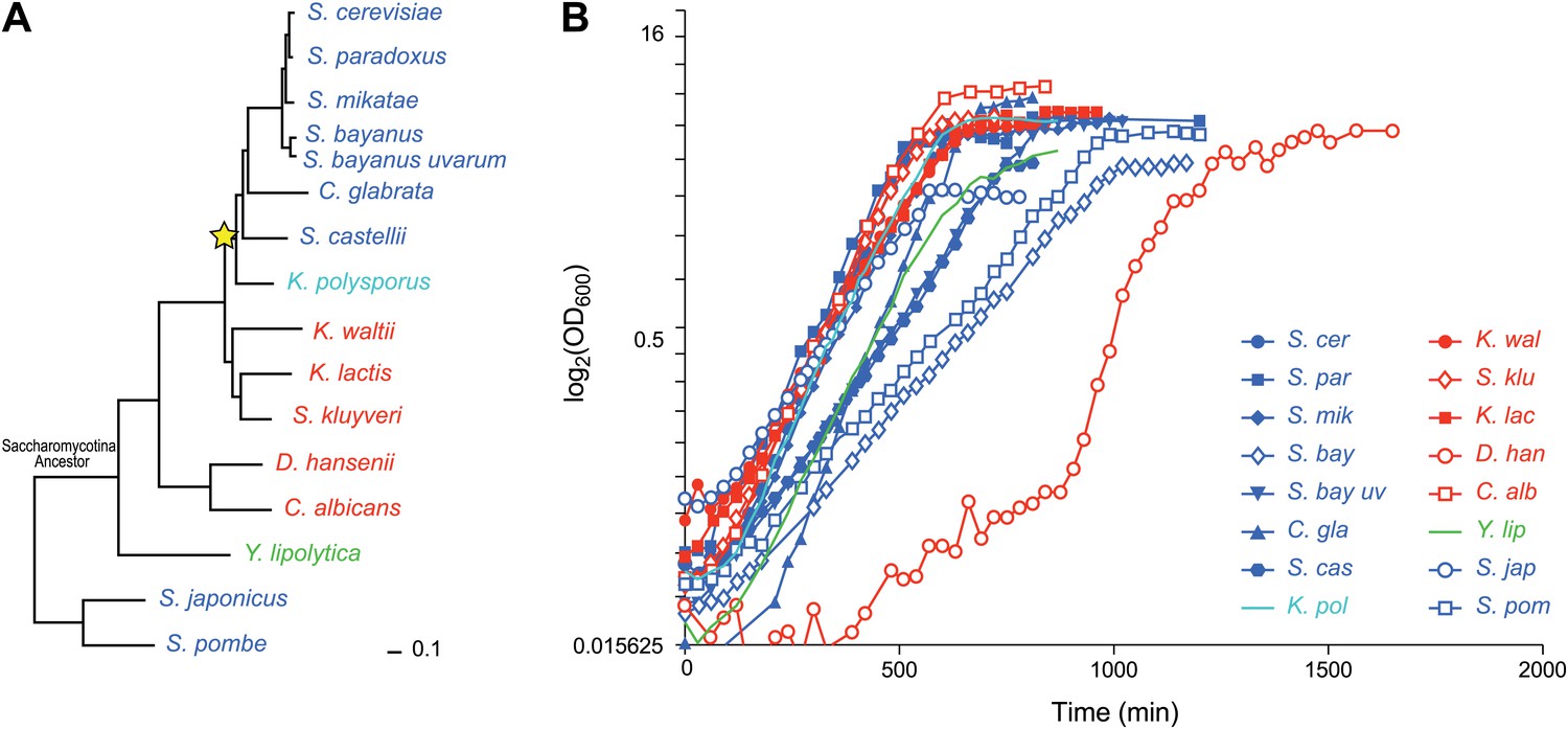
Ascomycota species in this study.
(A) A phylogenetic tree of the 15 Ascomycota species in the study. Dark blue: respiro-fermentative; red: respiratory; green: obligate respiratory; light blue: intermediate between respiro-fermentative and respiratory. Star: a Whole Genome Duplication event (WGD). (B) Growth rate (log(OD)600, y axis) of each species over time (y axis) during growth in the novel rich medium used in this study (see ‘Materials and methods’).
-
Figure 1—source data 1
Evolutionary distance across the phylogeny of 15 species.
Shown are the estimated branch lengths using PAML for our panel of 15 species. Each ’Sample’ represents the estimated branch length using a random subset of 1000 uniform orthogroups and the ‘Mean’ and ‘Stdev’ show the mean and standard deviations of these estimations.
- https://doi.org/10.7554/eLife.00603.004
Figure 2 with 1 supplement
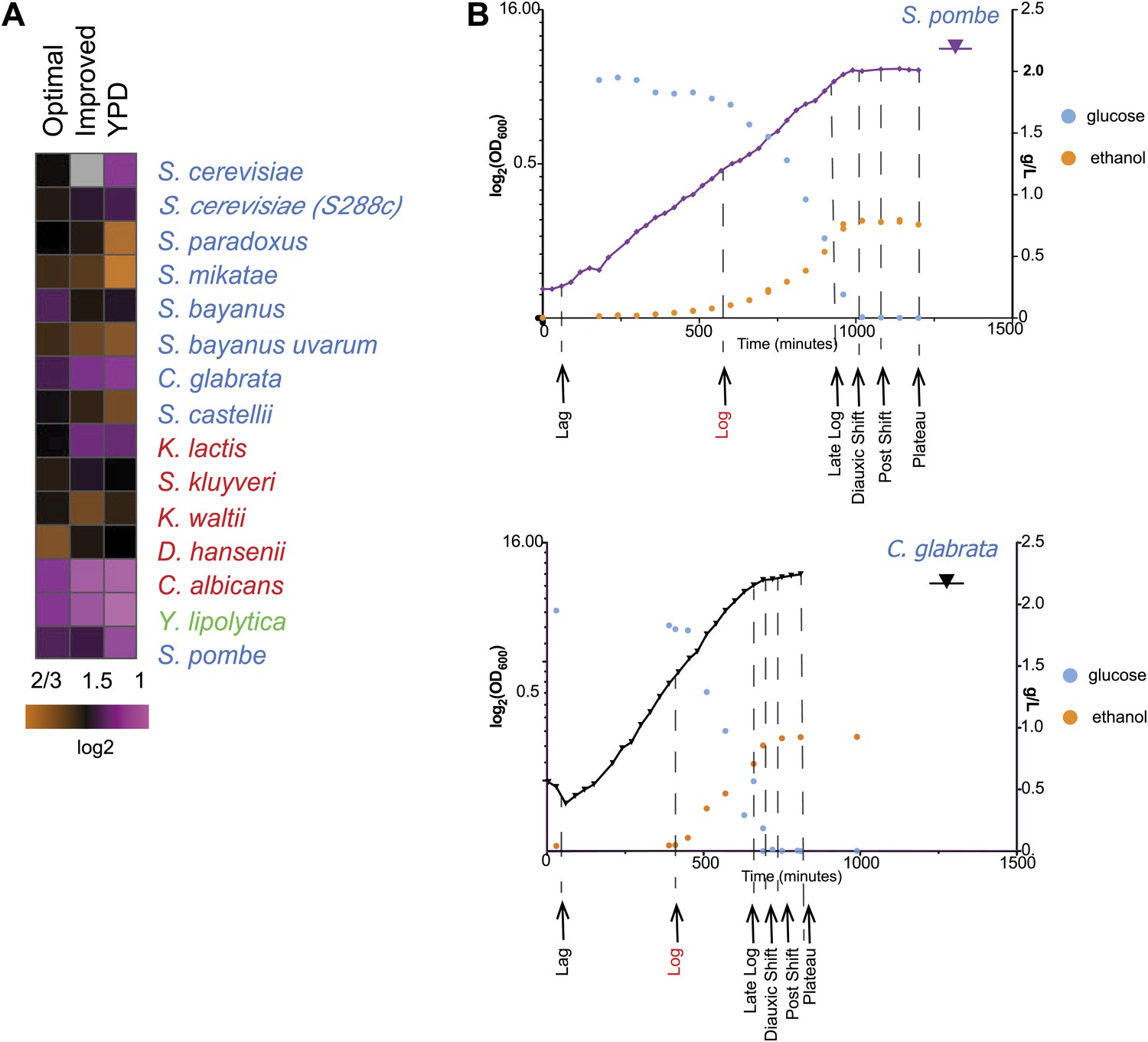
Growth of species in published and novel growth media.
(A) Performance of species in our optimized medium vs YPD medium, a common medium for S. cerevisiae. Shown are normalized saturation coefficients (log2(OD600) during a 24-hr growth period, a measure of accumulated biomass) of each species (‘Media tests’ under ‘Materials and methods’) in our panel (rows) in three media (columns). (B) Choosing ‘physiologically comparable’ time points. Our experiments compare ‘physiologically analogous’ time points across all species (see ‘Materials and methods’). For example, shown is the growth curve (x axis: time, minutes; y axis: growth rate, in log2(OD600) and glucose levels (g/L, blue) and ethanol levels (g/L, orange) for the relative slow growing species S. pombe (left) vs the growth curve for the faster growing C. glabrata (right). Biological samples from each species were taken at the time points indicated by arrows. The Log phase time point (shown in red) used as the reference for microarray analysis.
Figure 2—figure supplement 1
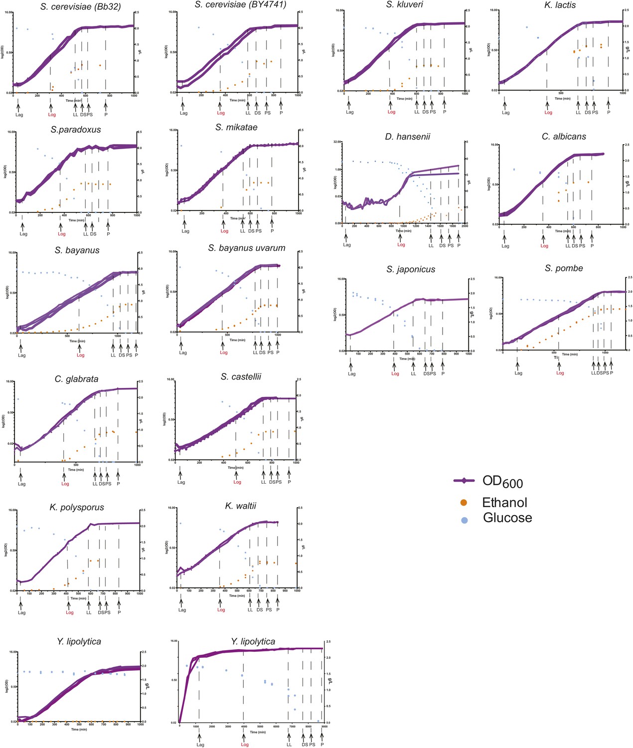
Phenotypic characterization of each species.
Shown are the growth curves (log2(OD600), purple), glucose levels (g/L, blue) and ethanol levels (g/L, orange) of two biological replicates for each species. Species name is noted on top of each panel. Y. lipolytica did not consume glucose despite a normal sigmoidal growth curve (left), presumably due to a preference to consume lipids as a carbon source. When the duration of the experiment was extended (right), this species consumed the glucose in the medium. Biological samples from each species were taken at the time points indicated by arrows at Lag, Log, Late log (LL), diauxic shift (DS), post-shift (PS) and plateau (P). The Log phase time point (shown in red) used as the reference for microarray analysis.
Figure 3 with 1 supplement
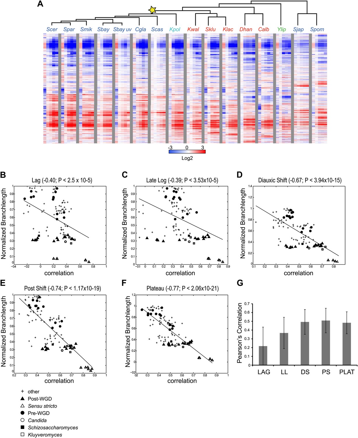
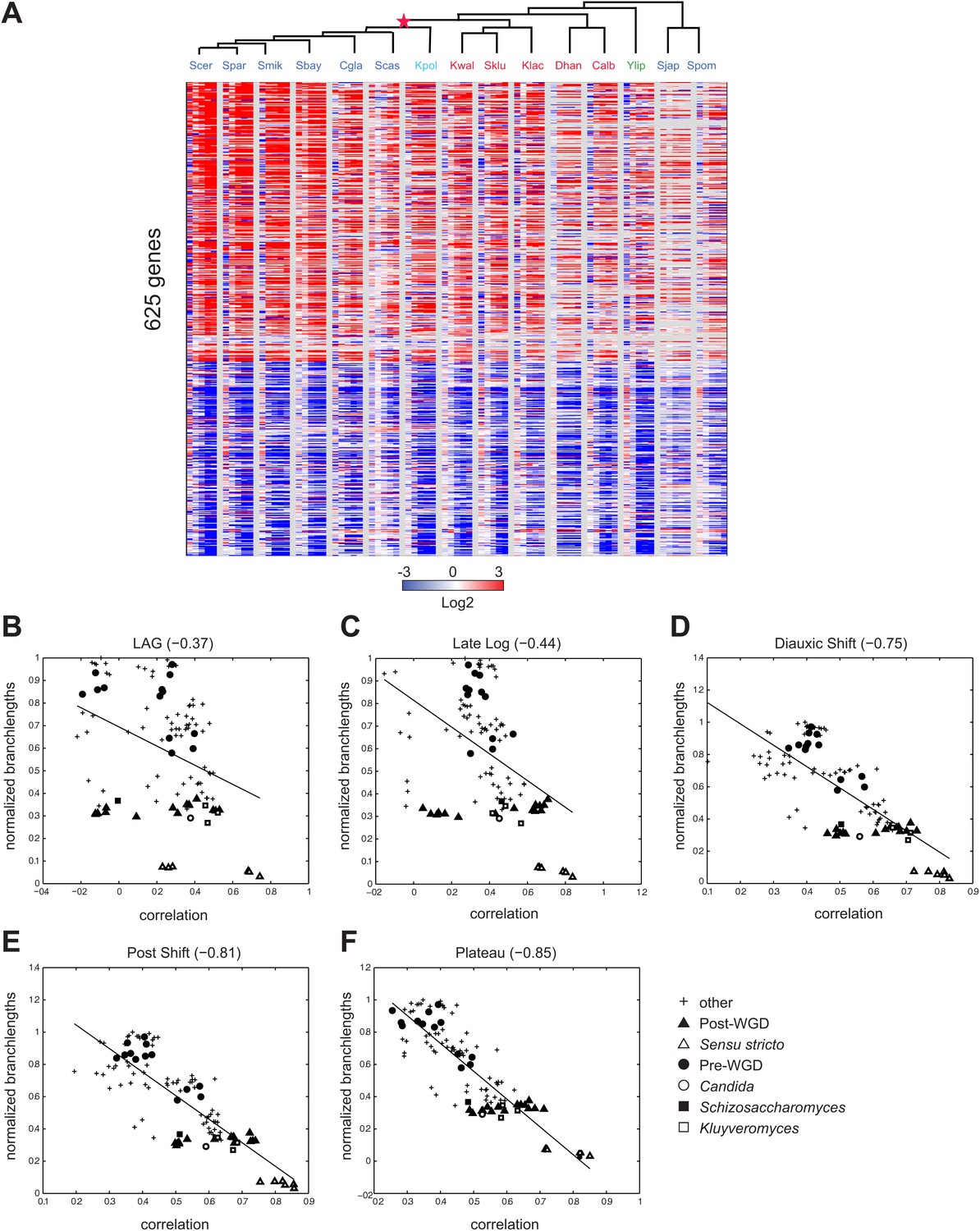
Divergence in global expression profiles correlates with phylogenetic distance.
(A) A comparative transcriptional compendium during growth on glucose. Shown are transcriptional profiles measured for each species (tree, top), at six time points (columns) during growth on glucose: Lag, Late Log, Diauxic Shift, Post Shift and Plateau (left to right). Genes (rows) are matched based on orthology and clustered (‘Materials and methods’). Red: induced; blue: repressed; white: no change; grey: ortholog absent in species. (B)–(F) Correlation in expression decreases with phylogenetic distance. Shown are scatter plots relating—for each pair of species—their estimated phylogenetic distance (y axis) and the correlation between their matching global expression profile (x axis) at a matching physiological time point (noted on top). The legend shows the clade to which the pair belongs (if the same) or ‘other’ (if from different clades). Branch length was scaled by the maximum branch length to range from 0 to 1. (B) Lag, (C) Late Log (LL), (D) Diauxic Shift (DS), (E) Post Shift (PS), (F) Plateau (PLAT). The line in each plot is the least squares fit. (G) Shown is the average Pearson’s correlation between pairs of species of the global expression profiles for each physiological time point.
-
Figure 3—source data 1
Experimental design and correlation among biological replicates.
Shown are the number of biological replicates per species per time point sampled, and the number of pairwise calculations used to calculate the correlation among biological replicates and the standard deviation.
- https://doi.org/10.7554/eLife.00603.009
Figure 3—figure supplement 1
Conservation of growth-rate regulated gene expression.
(A) Expression of growth genes across species. Shown are the expression profiles across all species (major columns) and time points (lag to plateau) for gene orthologs (rows) whose expression was previously positively (257) and negatively (368) correlated with growth rate (at 1.5 standard deviation) in S. cerevisiae by Brauer et al. (2008). Heatmap is laid out as in Figure 3. (B)–(F) Correlations in expression profiles are maintained when growth genes are excluded. Shown are scatter plots relating—for each pair of species—their estimated phylogenetic distance (Y axis) and the correlation between their matching global expression profile with the growth-rate regulated genes removed (X axis) at a matching physiological time point (noted on top). The legend shows the clade to which the pair belongs (if the same) or ‘other’ (if from different clades). Branch length was scaled by the maximum branch length to range from 0 to 1. (B) Lag; p≤1.14 × 10⁻⁴, (C) Late Log (LL); p≤2.45 × 10⁻⁴, (D) Diauxic Shift (DS); p≤1.5 × 10⁻²⁰, (E) Post Shift (PS); p≤8.22 × 10⁻²⁶, (F) Plateau (PLAT); p≤2.69 × 10⁻³⁰. The line in each plot is the least squares fit.
Figure 4
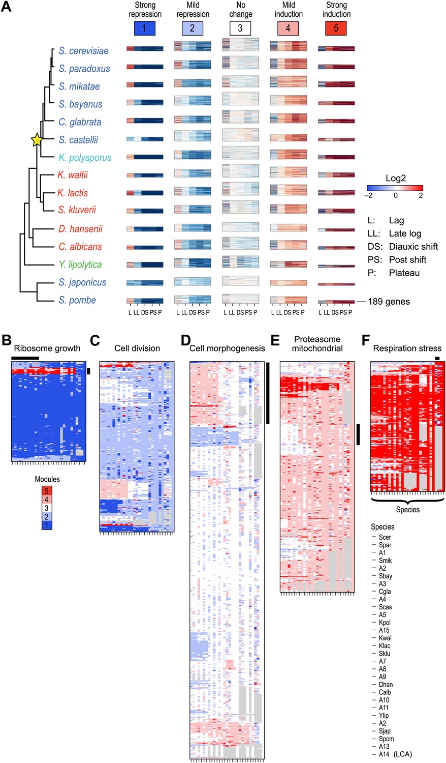
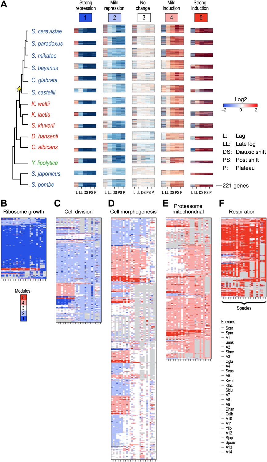
Arboretum reconstruction of expression module evolution (Analysis 1).
(A) Five expression modules identified by Arboretum in the transcriptional response to glucose depletion. Each row corresponds to a species (tree, left) and each major column to a module (1–5, labels top). Module labels are color coded by the regulation of the module’s genes following depletion, as noted on top, from bright blue (Module 1) for strong repression to bright red (Module 5) for strong induction. Each module’s height is proportional to the number of genes in the module. The five columns in each module are the expression levels at lag (L), late log (LL), diauxic shift (DS), post-shift (PS), and plateau (P) relative to mid-log phase. Red: induced; blue: repressed; white: no change. (B)–(F) Module assignments in all extant and ancestral species (see Figure 5B for ancestral node assignment). Each matrix corresponds to the genes in one of the five modules in the LCA (A14) (B: Module 1; C: Module 2; D: Module 3; E: Module 4; F: Module 5), and shows the module assignment of these genes in each of the extant and ancestral species from S. cerevisiae (leftmost column) to the LCA (rightmost column). The biological functions listed at the top of each module are representative labels chosen based on Gene Ontology terms enriched in all species in that module (Supplementary file 1). The range of FDR p values and fraction of genes in each module are as follows: Module 1: Ribosome biogenesis, p<5.28 × 10−48 to 1.25 − 10−119, fraction 37.3–61.6%. Module 2: cell division, p-value<3.51 × 10−02 to 4.52 × 10−02, fraction 9–33.6%. Module 3: cell morphogenesis, p<4.64 × 10−02 to 4.95 × 10−02, fraction 6.5–81%. Module 4: mitochondrial, p<3.20 × 10−02 to 4.90 × 10−02, fraction 2.4–37.9%; proteasome, p<3.85 × 10−04 to 3.97 × 10−02, fraction 1.6–15%. Module 5: respiration p<4.77 × 10−02 to 4.8 × 10−02, fraction 32.6–58.9%; response to stress, p<4.75 × 10−02 to 4.86 × 10−02, fraction 2.6–13.7%. Module assignment in each species is marked by a color code, as in the top of panel A (bright blue: Module 1; light blue: Module 2; white: Module 3; pink: Module 4; red: Module 5). Species are ordered by post-fix ordering (left-child, right-child and parent) of the species tree, as marked on the legend (bottom). Black bars indicate points of phylogenetically coherent divergence in expression of orthologous genes, as discussed in the text.
-
Figure 4—source data 1
Orthogroups included in the Aboretum run for analysis 1.
Shown are the genes used for Arboretum run excluding orthogroups with duplications (Analysis 1). Each column corresponds to an extant species. The string ‘Dummy’ separates the genes from different modules.
- https://doi.org/10.7554/eLife.00603.012
Figure 5
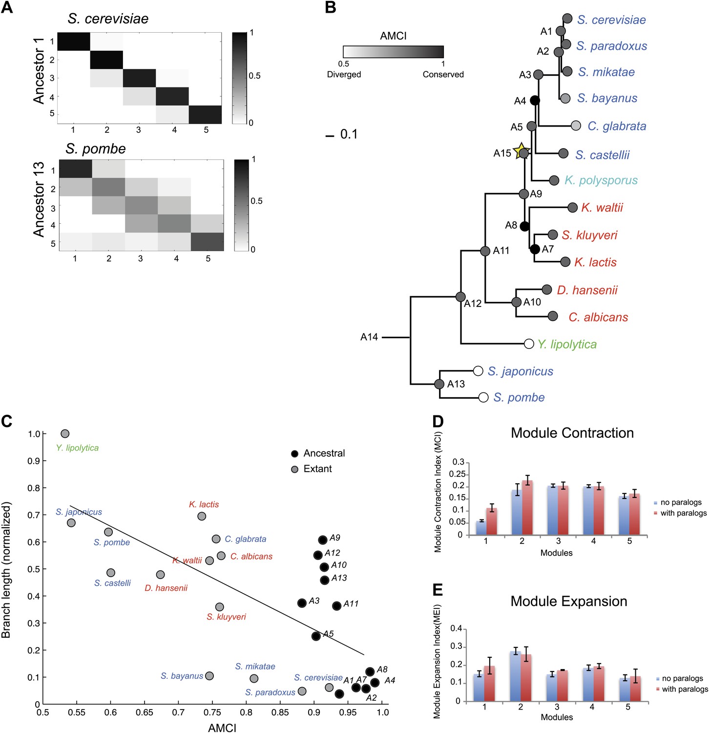
Conservation of modular organization.
(A) Module transition matrices. Shown are examples of transition matrices estimated by Arboretum for two species (S. cerevisiae, top and S. pombe, bottom). Each matrix specifies, for each module in each child species (columns), the probability with which a gene conserved its module assignment in that species’ immediate ancestor (rows), or was reassigned to another module. Columns: modules of the child species, rows: modules of the ancestor species. Probabilities are color coded from black (1) to white (0). Strong diagonal elements indicate high conservation with the immediate ancestor. The AMCI is calculated as the mean of the diagonal entries. (B) The Ancestral Module Conservation Index (AMCI). Shown is the AMCI, ranging from 0: least conserved (white circles) to 1: most conserved (black circles), for each extant and ancestral species. Tree is drawn to scale and species are color coded by carbon lifestyle as in Figure 1A. (C) AMCI decreases with increased phylogenetic distance. Shown is a scatter plot of the relationship, for each extant (grey) and ancestral (black) species, between its phylogenetic distance to its immediate ancestor (branch length, y axis) and its AMCI (x axis). Branch length is scaled by the maximum value to range between 0 and 1. The correlation between branch length and AMCI is −0.68 (p≤1.13 −× 10−4). The regression line is plotted. (D) and (E) Expansion and contraction of modules. Shown are the mean Module Contraction Index (MCI, D) and mean Module Expansion Index (MEI, E) for each Arboretum module (x axis), based on the proportion of genes that respectively leave or join each module at each phylogenetic point. Blue and red indicate the modules from Arboretum runs with only no duplicates (no paralogs) and including duplicates (with paralogs), respectively. Error bars were estimated from five Arboretum runs with different initializations.
Figure 6 with 1 supplement
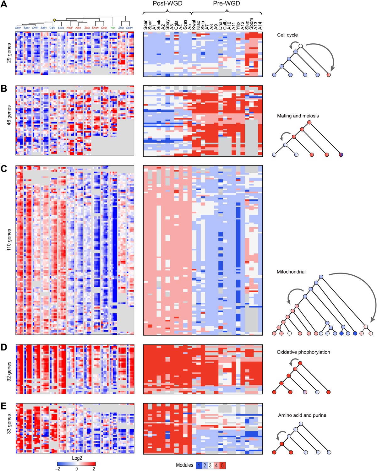
Conservation and rewiring of coherent functions across modules.
Shown are expression (left), Arboretum module assignments (middle) and a cartoon of the phylogenetic transition (right) for gene sets with coherent phylogenetic patterns. Each expression matrix is formatted as in Figure 3A, and each module assignment matrix as in Figure 4B–F. (A) Cell cycle genes, (B) mating and meiosis related genes, (C) mitochondrial genes, (D) oxidative phosphorylation genes, (E) amino acid and purine metabolism genes. Each module shows all the genes with a given phylogenetic pattern, and their labels (e.g., mitochondrial) were manually generated based on enrichment of GO terms.
Figure 6—figure supplement 1
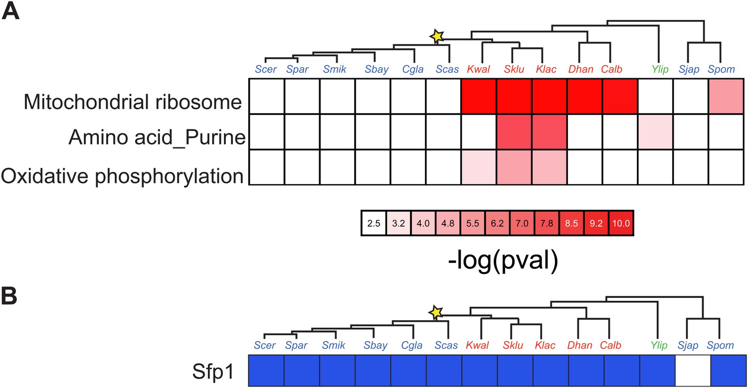
Enrichment of Sfp1 binding sites.
(A) in the promoters of genes with specific functions. Shown are the negative logarithm of the p value (red intensity) for a test of enrichment (see ‘Materials and methods’) of the Sfp1 motif in the promoters of genes for mitochondrial, purine and amino acid metabolism and oxidative phosphorylation functions (rows), across the 15 species (columns). (B) Shown is the enrichment of the Sfp1 binding sites (FDR < 0.05) in Arboretum Module 1 (‘growth module’).
Figure 7
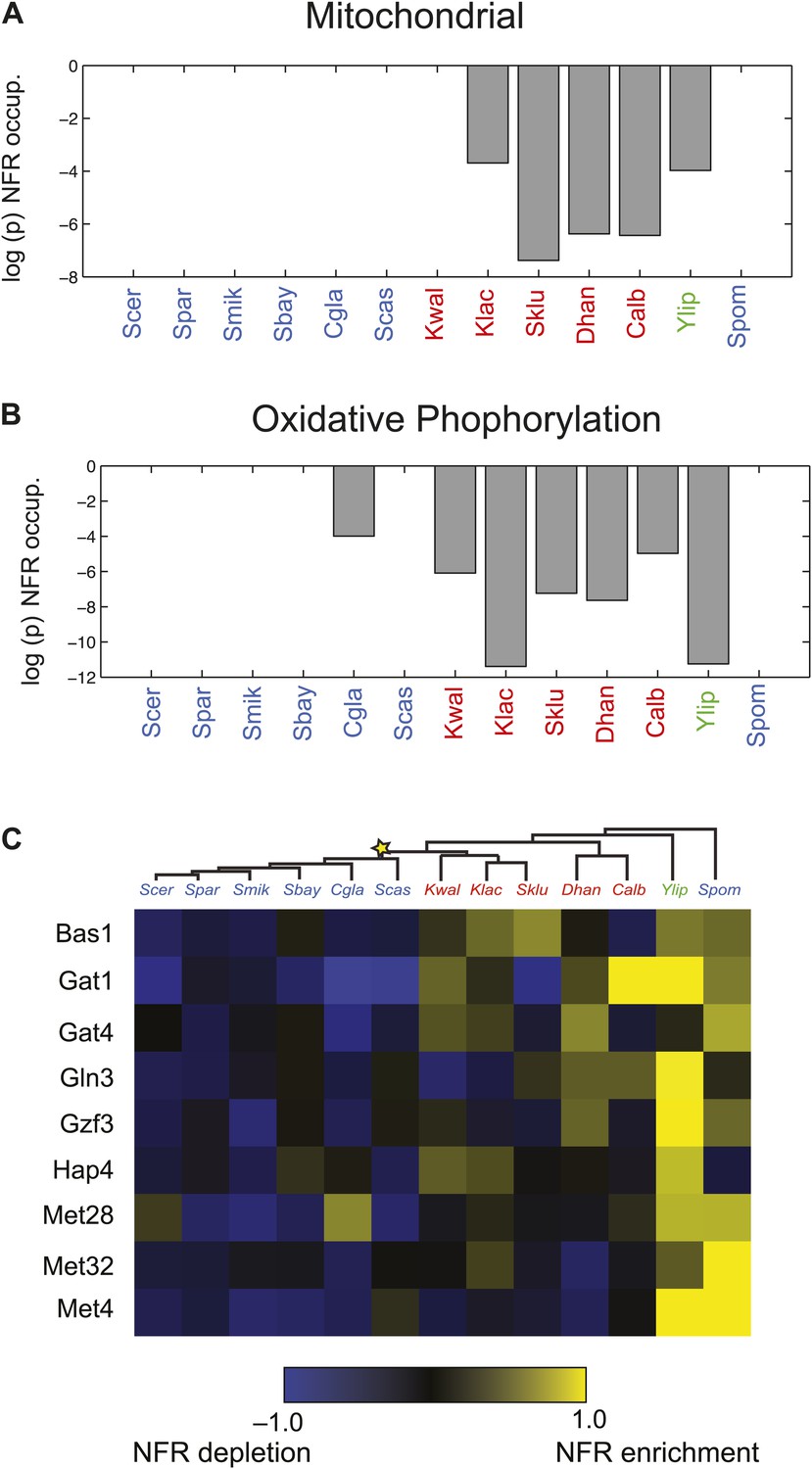
Changes in chromatin organization in mitochondrial, oxidative phosphorylation and amino acid metabolism genes.
Shift in NFR occupancy in re-wired respiratory genes (A and B). Shown are the logarithm of the p value of the KS-test (y axis) used to test if the genes in a given set (mitochondrial genes, A, and oxidative phosphorylation genes, B) have a significantly lower nucleosome occupancy at their 5′NFRs than that of all genome genes in each of 13 species (x axis) with nucleosome positioning data from Tsankov et al. (2010) and Xu et al. (2012). (C) Evolutionary repositioning of binding sites for key amino acid TFs relative to NFRs. For each of 13 species (columns, tree), shown are the enrichment (yellow) or depletion (blue) in NFRs of binding sites for several amino acid and purine metabolism TFs (rows) whose sites are depleted from NFRs in post-WGD species and enriched in pre-WGD species. The intensity of the color is proportional to the z-score estimated for each regulator from the fraction of all its binding sites that are in the NFR. Each row is centered by its mean value (see ‘Materials and methods’).
Figure 8
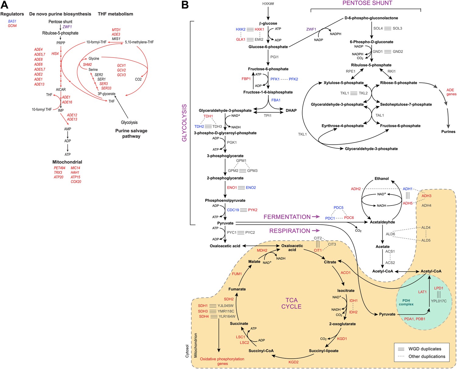
Purine and amino acid metabolic pathways are linked to carbon metabolism.
(A) Shown are the set of metabolic reactions in S. cerevisise associating purine biosynthesis and salvage and amino acid metabolism with carbon metabolism, and two key transcriptional regulators (left). Mitochondrial genes link respiration to purine metabolism. Glycolysis is linked to purine salvage by the metabolic intermediate 3-P-glycerate. De novo purine metabolism is linked to the pentose shunt through ribulose-5-phosphate. The genes in red are induced post-shift in S. cerevisiae and other post-WGD species, but their orthologs are repressed in pre-WGD species. Both Schizosaccharomyces species have three copies of ZWF1 (purple) that are strongly induced. (B) Shown are the major carbon pathways involved in the fermentation or respiration of glucose and their interconnectivity. Both WGD and other duplicate genes in each pathway are indicated. The genes in red are induced post-shift in S. cerevisiae and most of the other post-WGD species while those in green are repressed similar to their pre-duplication orthologs. Differences in trans regulators may further contribute to the reassignment of their targets between modules. While many of the regulators of glucose repression in S. cerevisiae are present across the phylogeny (Flores et al., 2000), the regulation of some has changed at the WGD and at the ancestor of the Schizosaccharomyces, consistent with the reassignment of their targets. For example, the glucose repressing MIG genes and the TUP1-CYC8 complex are strongly repressed following glucose depletion in most post-WGD species, whereas some respiration activators are strongly induced (CAT8 and HAP2,4,5 and SIP2 post-WGD, HAP2, MOT3, and SIP2 in S. pombe, data not shown). We observed no such changes in the expression of known regulators of amino acid and purine metabolism (data not shown). In some cases, duplication of key regulators followed by reassignment to a new module may have further contributed to new regulatory functions. For example, TPK1 and TPK3 are two WGD-derived paralogs encoding catalytic subunits of PKA, a major regulator of carbohydrate metabolism and stress responses (Zaman et al., 2008). TPK1 in strongly induced in the sensu stricto species, as is the single TPK gene in the Schizosaccharomyces. TPK3 is repressed in those species, conserving the expression pattern of its ortholog in all the respiratory pre-duplication species (data not shown).
Figure 9
Arboretum reconstruction of expression module evolution in the presence of paralogous genes (Analysis 2).
(A) Five expression modules identified by Arboretum in the transcriptional response to glucose depletion, when paralogous genes are included in the run. Each row corresponds to a species (tree, left) and each major column to a module (1–5, labels top). Modules labels are color coded by the regulation of the module’s genes following depletion, as noted on top, from bright blue (Module 1) for strong repression to bright red (Module 5) for strong induction. Each module’s height is proportional to the number of genes in that module. The five columns in each module are the expression levels at lag (L), late log (LL), diauxic shift (DS), post-shift (PS), and plateau (P) relative to mid-log phase. Red: induced; blue: repressed; white: no change. (B)–(F) Module assignments of all extant and ancestral species. Each matrix corresponds to the genes in one of the five modules in the LCA (B: Module 1; C: Module 2; D: Module 3; E: Module 4; F: Module 5), and shows the module assignment of these genes in each of the extant and ancestral species from S. cerevisiae (leftmost column) to the LCA (rightmost column). The biological functions listed at the top of each module are general classifiers based on Gene ontology terms enriched in all species in that module (Supplementary file 2). The range of FDR p values and fraction of genes in each module are as follows: Module1: ribosome biogenesis, p<1.07 − 10−52 to 1.56 × 10−112, fraction 32–53%. Module2: cell division, p<3.13 × 10−02 to 4.69 × 10−02, fraction 10.2–32%. Module 3: cell morphogenesis, p<4.48 × 10−02 to 4.56 × 10−02, fraction 22–78.7%. Module 4: mitochondrial, p<2.47 × 10−02 to 3.36 × 10−02, fraction 2.3–36.2%; proteasome, p<2.7 × 10−03 to 5.48 × 10−03, fraction 1.3–13.1%. Module 5: respiration, p<4.2 × 10−02 to 4.43 × 10−02, fraction 34.9–55%. Module assignment in each species is marked by a color code, as in the top of panel a (bright blue: Module 1, light blue: Module 2, white: Module 3, pink: Module 4, red: Module 5). Species are ordered by post-fix ordering (left-child, right-child and parent) of the species tree, as marked on the legend (bottom).
-
Figure 9—source data 1
Orthogroups included in the Aboretum run for analysis 2.
Shown are the genes used for Arboretum run including orthogroups in Analysis 1 as well as orthogroups with one duplication event (Analysis 2). The string ‘Dummy’ separates the genes from different modules.
- https://doi.org/10.7554/eLife.00603.019
Figure 10
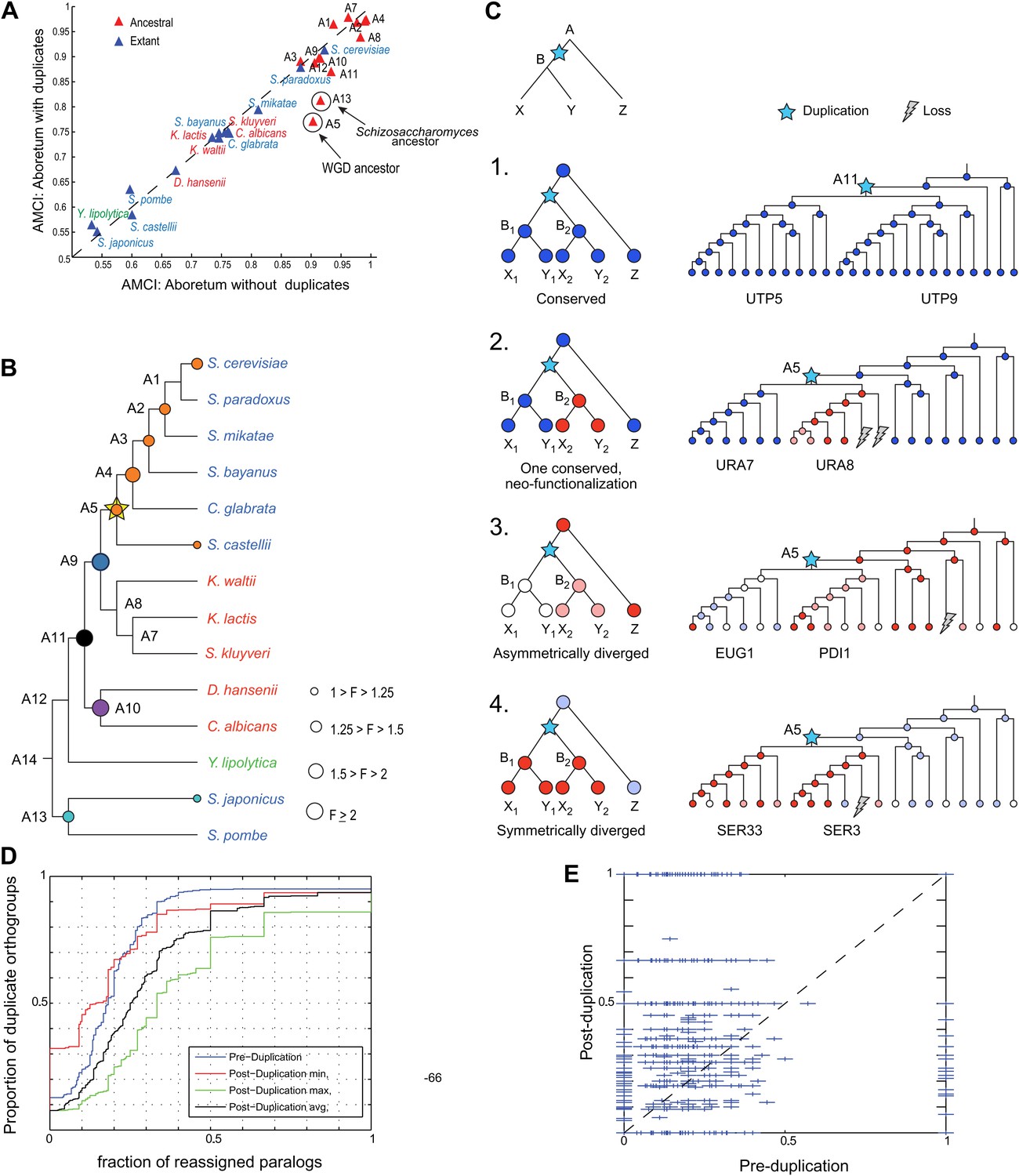
Regulatory evolution of paralogous genes.
(A) Paralogous genes contribute to regulatory divergence. Shown in a scatter plot of the AMCI values for each extant (blue) and ancestral (red) species as estimated by Arboretum in a run without paralogs (Analysis 1) (y axis) vs a run with paralogs (x axis). Inclusion of paralogous genes lowers the AMCI, especially at the WGD and Schizosaccharomyces ancestors (arrows). (B) Enrichment of paralogous genes among reassigned genes. Shown is for each species (ancestral and extant) the fold enrichment (F) of paralogs (circle size) among genes reassigned at that species. Only points at which there are significantly more paralogs that switch than expected by chance are shown (Hyper-geometric p<0.05). Circles are colored by the phylogenetic point of gene duplication (cyan: A13, black: A11, purple: A10, blue: A9, white: WGD ancestor A5). (C) Four possible regulatory fates of paralogous genes following duplication, relative to their immediate pre-duplication ancestor. Left: cartoon gene trees (left) and illustrative examples from our analysis (right) representing the module assignment (circles) of each paralog and their pre-duplication ortholog in each extant and ancestral species. Module assignment is color coded as in Figure 3 (Bright blue, light blue, white, pink, red from Module 1 to 5, respectively). Star: gene duplication. Lightning rod: gene loss. (1) Conserved: both paralogs (UTP5 and UTP9) conserve the ancestral assignment (Module 1); (2) Neo-functionalization: one paralog (URA7) maintains the ancestral assignment (Module 1) and the other (URA8) is assigned to a different module (Module 5); (3) Asymmetric divergence: both paralogs (EUG1, PDI1) are reassigned to distinct modules (Module 3, Module 4) than the ancestral one (Module 5). (4) Symmetric divergence: both paralogs (SER3, SER33) are reassigned to the same module (Module 5), distinct from the ancestral one (Module 1). (C) Cumulative distribution of module reassignment of genes before and after their duplication. Because after duplication there are two paralogs, each with its own re-assignment value, we compare the minimum (red, p<1 × 10⁻⁴), maximum (green, p<1 × 10−66), and average (black, p<1 × 10⁻¹⁸) of the number of re-assignments after duplication, with the re-assignments before duplication (blue). (D) Scatter plots showing for each gene its degree of module reassignment before duplication (x axis) vs the average degree of module reassignment of the two paralogs after duplication (y axis). All module reassignments for a gene are normalized by the number the species in which the gene is present (‘Materials and methods’).
-
Figure 10—source data 1
Gene Ontology enrichment in sets of duplicate genes that diverged from the pre-duplication ancestor.
Shown are the GO processes enriched in gene sets that switch their module assignment from their pre-duplication module. Each row corresponds to a GO process (column 1), and the subsequent columns indicate the phylogenetic point of duplication and numbers used to estimate the p value from the Hyper-geometric test.
- https://doi.org/10.7554/eLife.00603.021
Figure 11
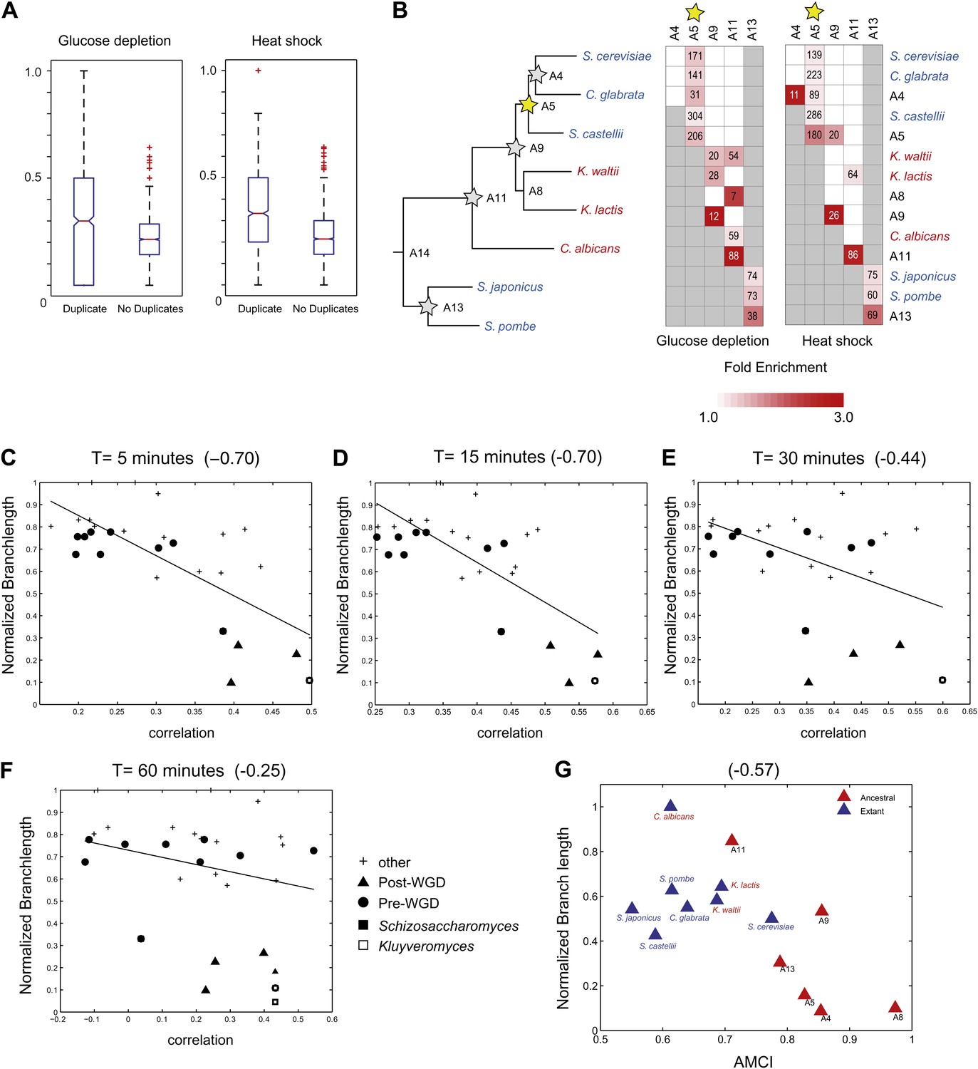
Similar evolutionary patterns in glucose depletion and heat shock.
(A) Increased re-assignment of paralogous genes. Box-plots showing the fraction of module re-assignments for genes from orthogroups with duplication events (Duplicate, left) and without duplication events (Singleton, right). Red plus: outliers that are ±2.7 SD from the mean. (B) Enriched re-assignment of paralogous genes at different phylogenetic points. Shown are the fold enrichment of paralogous genes among all the reassigned genes (red, scale bar) at different phylogenetic points (rows) for duplicates that arose at different ancestors (columns) for heat shock (left) and glucose depletion (right). The number in each cell represents the number of paralogous genes that arose at a given phylogenetic point (column) and were reassigned at a phylogenetic point (row). Numbers and fold enrichment are marked only at points with significantly more paralogs that are reassigned than expected by chance (Hypergeometric p<0.05). (C)–(F) correlation in expression decreases with phylogenetic distance. Shown are scatter plots relating—for each pair of species—their estimated phylogenetic distance (y axis) and the mean correlation between their matching global expression profiles (x axis) at matching time points (labeled on top). Legend shows the clade to which the pair belongs (if the same) or ‘other’ (if from different clades). Branch length was scaled by the maximum branch length to range from 0 to 1. The line is the least squares fit. The Pearson correlation coefficient is shown on top (C: p≤2.88 × 10⁻⁵; D: p≤2.86 × 10⁻⁵; E: p≤0.018; F: p≤0.19). (G) Module divergence scales with phylogenetic distance. Shown is a scatter plot of the relationship, for each extant (blue) and ancestral (red) species, between its phylogenetic distance to its immediate ancestor (branch length, y axis) and its AMCI (x axis). Branch length is scaled by the maximum value to range between 0 and 1. The correlation between branch length and AMCI is shown at top (p≤0.033).
Figure 12
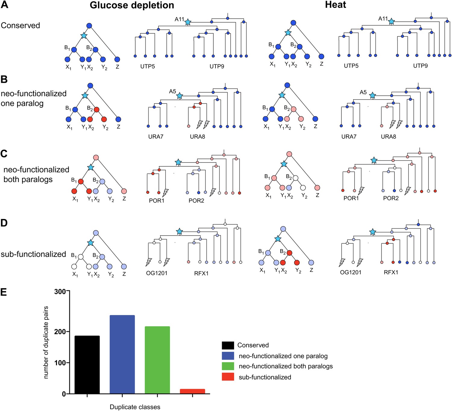
Regulatory evolution of paralogous genes in glucose depletion and heat shock.
(A)–(D) several regulatory fates of paralogous genes following duplication, relative to their immediate pre-duplication ancestor in each of glucose depletion and heat shock. For each condition shown are cartoon gene trees (left) and illustrative examples from our analysis (right) representing the module assignment (circles) of each paralog and their pre-duplication ortholog in each extant and ancestral species. Module assignment is color coded as in Figure 3 (Bright blue, light blue, white, pink and red from Module 1 to 5, respectively). Star: gene duplication. Lightning rod: gene loss. (A) Conserved: both paralogs (UTP5 and UTP9) conserve the ancestral assignment (Module 1) in both responses; (B) Neo-functionalized, one paralog: one paralog (URA7) maintains the ancestral assignment (Module 1) and the other (URA8) is assigned to a different module (Module 5) in both responses; (C) Neo-functionalized, both paralogs: both paralogs (POR1, POR2) are reassigned to distinct modules than the ancestral one, but in different ways in each response. (D) Sub-functionalization: In glucose depletion, one paralog (RFX1) maintains the ancestral assignment (Module 2) and the other (OG1201) is reassigned (Module 3). This pattern is reversed in heat shock. (E) Number of paralogs pairs in each of the classes.
Figure 13
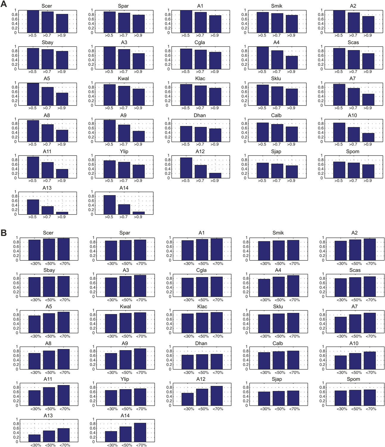
The per gene probability of Arboretum module assignments.
(A). Shown are the fraction of genes (y axis) that are assigned to the most likely module with probability of at least 0.5, 0.7 or 0.9 in each species (x axis). (B). Shown are the fraction of genes (y axis) whose probabilities of the second most likely assignment is less 30%, 50%, or 70% of the most likely assignment, that is q/p<x% where q is the probability of the second most likely assignment and p is the probability of the most likely assignment.
Figure 14 with 1 supplement
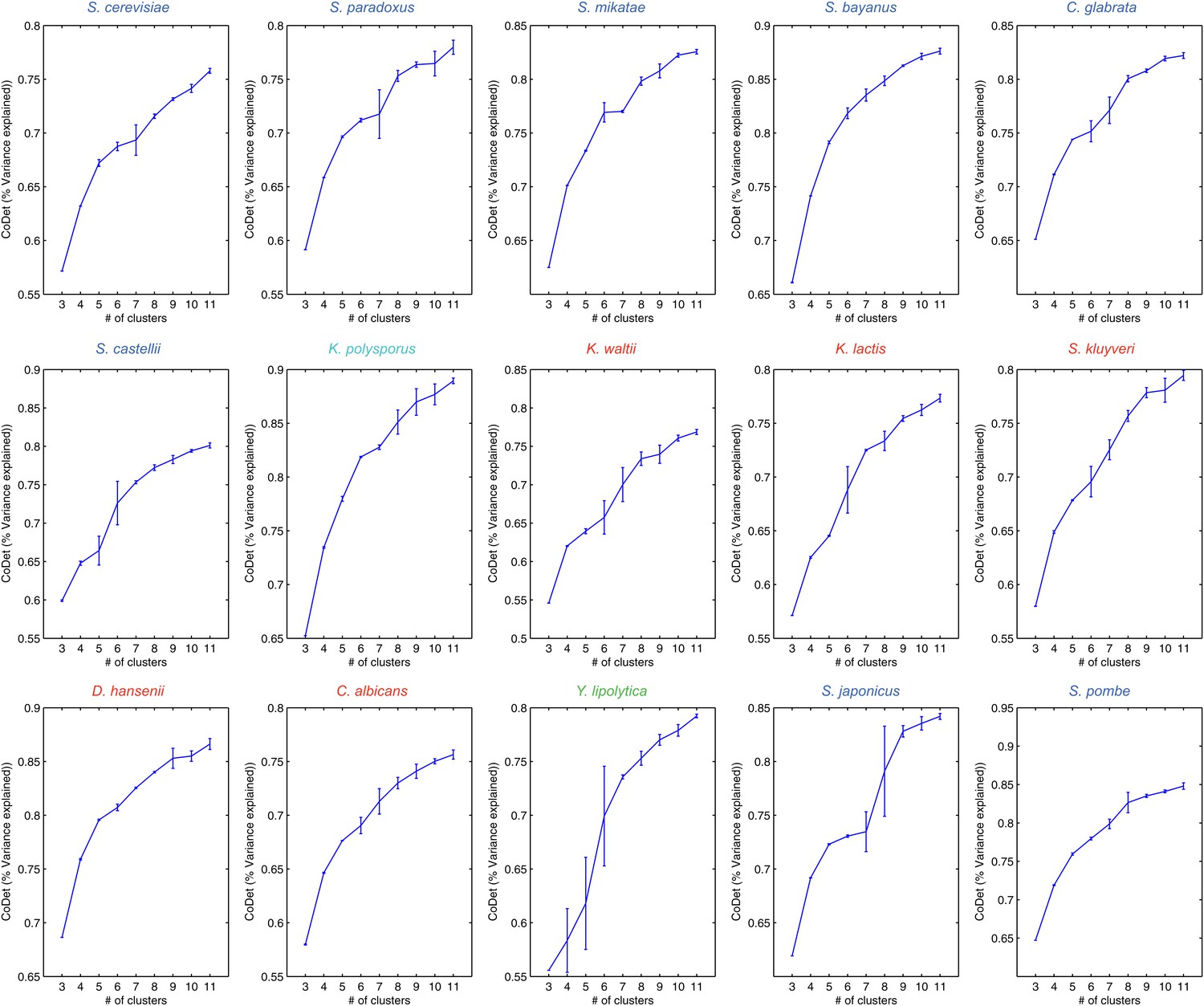
Variance captured in Arboretum modules as a function of the number of modules.
Shown are the mean and standard deviation of the coefficient of determination for each species, one per plot. Mean and standard deviation were calculated for different random initializations of Arboretum runs. Coefficient of determination (y axis) was measured for different values of the number of modules (x axis).
Figure 14—figure supplement 1
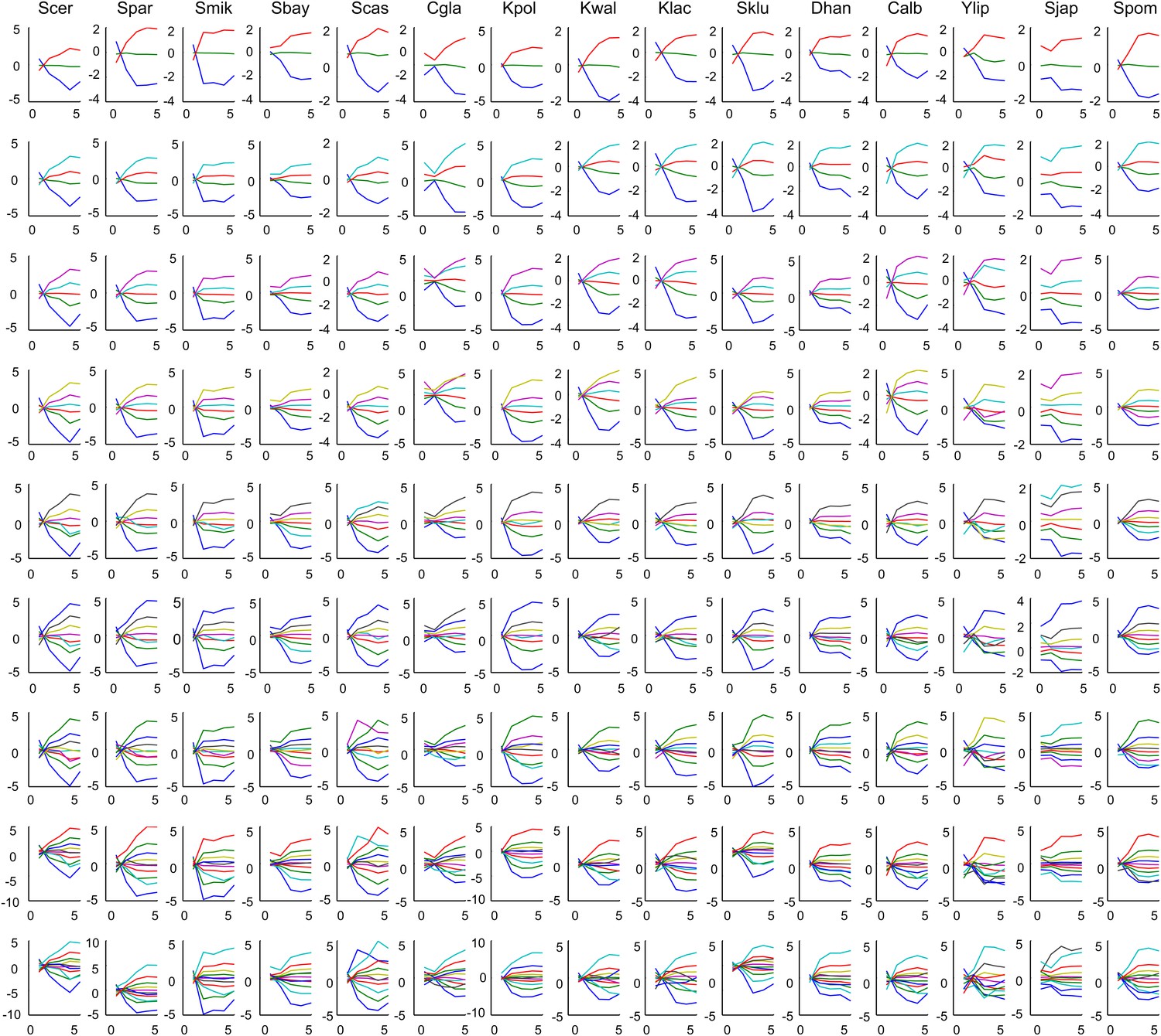
Mean expression of Aboretum modules as a function of different k values.
Each plot is the mean expression profile of a module. Each row corresponds to different k's and each column corresponds to a species.
Author response image 1
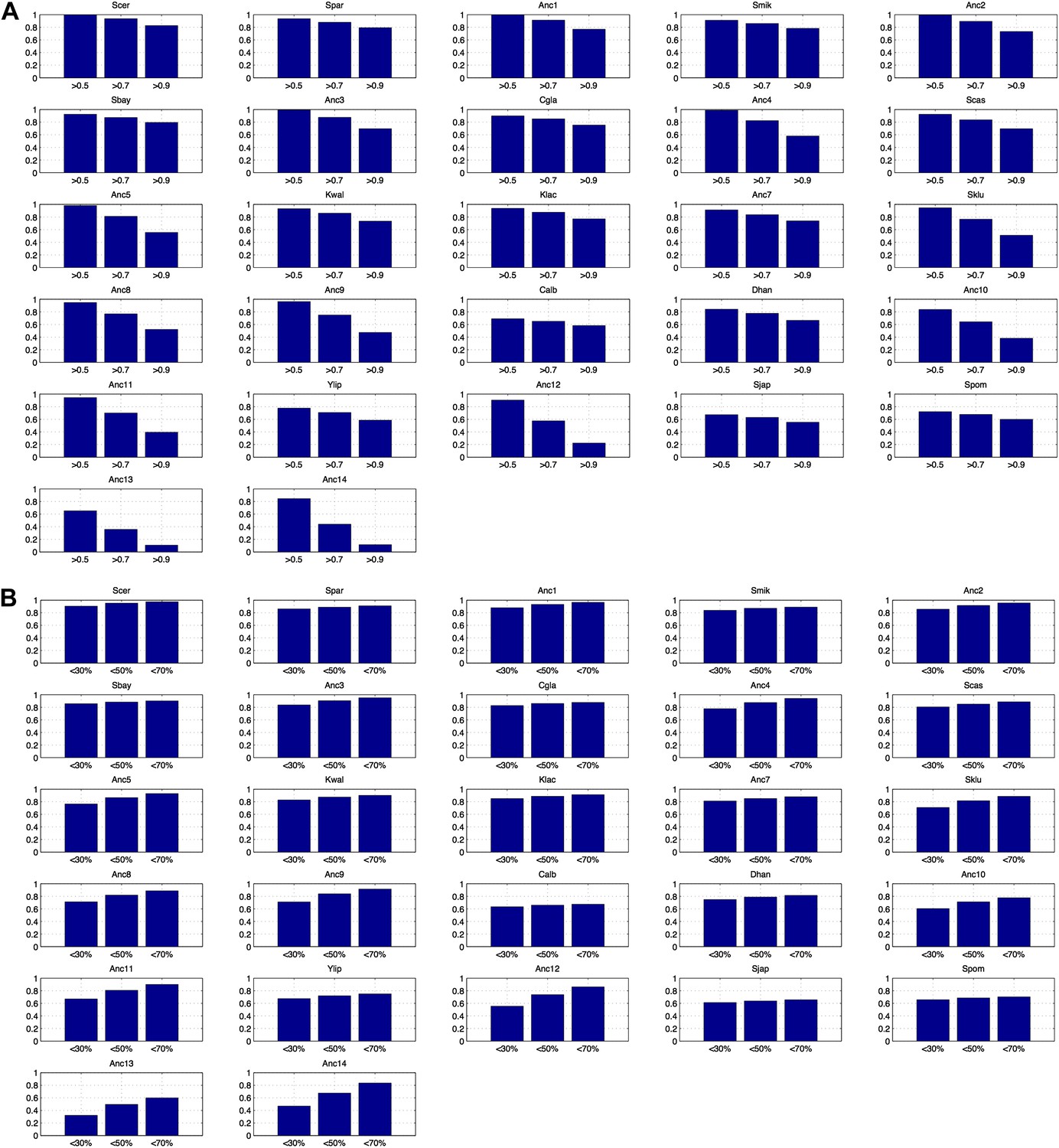
A. Shown are the fraction of genes (y-axis) that are assigned to the most likely module with probability of at least 0.5, 0.7 or 0.9 in each species (x-axis). B. Shown are the fraction of genes (y-axis) whose probabilities of the second most likely assignment is less 30%, 50%, or 70% of the most likely assignment, that is q/p <x% where q is the probability of the second most likely assignment and p is the probability of the most likely assignment.
Author response image 2
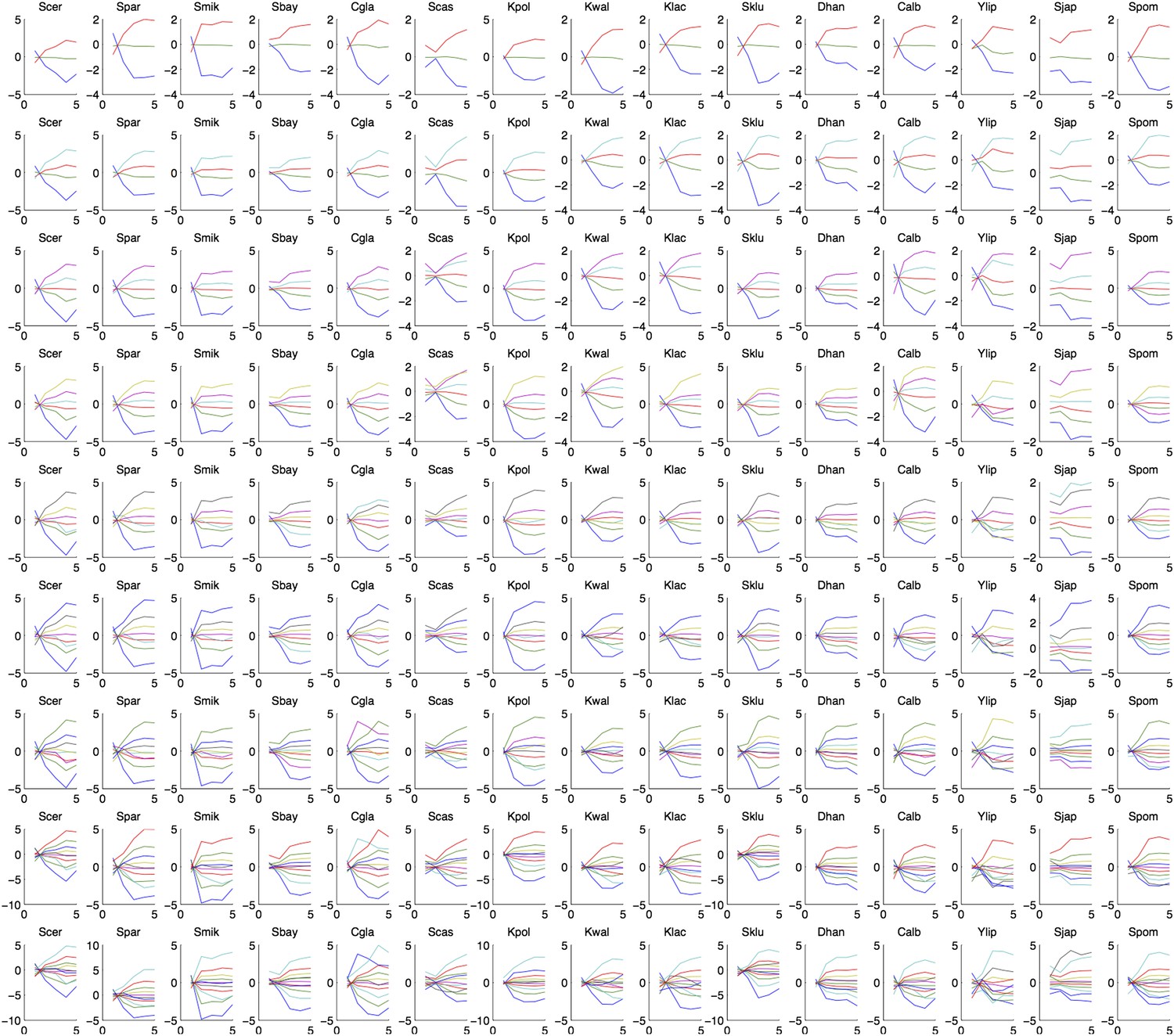
Each plot is the mean expression profile of a module. Each row corresponds to different k’s and each column corresponds to a species.
Author response image 3

Shown are expression heat maps of the 45 genes for which Arboretum inferred a lower module assignment in S. mikatae compared to S. bayanus. Each heat map shows the same 45 genes at different saturation levels log ratio −1 to 1 (top), −2 to 2 (middle), −3 to 3 (bottom).
Tables
Table 1
Number of genes and orthogroups
| Species | Total genes in species | Total genes on arrays | Total orthogroups on arrays | Total genes with tree*,† | Orthogroups available for analysis‡ | Genes available for analysis§ | Orthogroups analysis 1# | Genes analysis 1# | Orthogroups analysis 2¶ | Genes analysis 2¶ |
|---|---|---|---|---|---|---|---|---|---|---|
| S. cerevisiae | 6343 | 6257 | 4424 | 5508 | 4402 | 5464 | 2746 | 2746 | 3676 | 3964 |
| S. paradoxus | 5512 | 5504 | 4319 | 5256 | 4312 | 5244 | 2577 | 2577 | 3452 | 3720 |
| S. mikatae | 5697 | 5693 | 4251 | 5094 | 4251 | 5093 | 2513 | 2513 | 3382 | 3618 |
| S. bayanus | 5489 | 5483 | 4272 | 5191 | 4269 | 5188 | 2555 | 2555 | 3416 | 3679 |
| C. glabrata | 5338 | 5269 | 4126 | 4909 | 4119 | 4897 | 2534 | 2534 | 3394 | 3614 |
| S. castellii | 5693 | 5689 | 4277 | 5420 | 4257 | 5362 | 2574 | 2574 | 3461 | 3794 |
| K. polysporus | 5328 | 5324 | 4039 | 4539 | 4027 | 4525 | 2506 | 2506 | NA | NA |
| K. waltii | 5198 | 5194 | 4381 | 4849 | 4381 | 4848 | 2560 | 2560 | 3432 | 3497 |
| K. lactis | 5328 | 5323 | 4435 | 4888 | 4428 | 4879 | 2572 | 2572 | 3455 | 3537 |
| S. kluyveri | 5321 | 5320 | 4393 | 4879 | 4386 | 4865 | 2496 | 2496 | 3364 | 3444 |
| D. hansenii | 7938 | 6893 | 4050 | 4635 | 4034 | 4608 | 1903 | 1903 | 2551 | 2634 |
| C. albicans | 6163 | 6107 | 4858 | 5692 | 4858 | 5692 | 2324 | 2324 | 3110 | 3232 |
| Y. lipolytica | 6756 | 6672 | 4260 | 4886 | 4258 | 4874 | 2138 | 2138 | 2855 | 2921 |
| S. japonicus | 5297 | 5149 | 3863 | 4248 | 3861 | 4246 | 1878 | 1878 | 2487 | 2557 |
| S. pombe | 5068 | 5060 | 4208 | 4751 | 4208 | 4750 | 2001 | 2001 | 2487 | 2746 |
-
Shown are the total number of genes in each species (defined as the sum of genes on arrays and with orthology, ‘Materials and methods’). The number of genes, genes that have orthologs in another species, and the classes of genes that were measured on the species-specific arrays (1) total number of genes (2) total number of orthogroups (3) non-singleton (those present S. cerevisae and in at least one other species). Also shown is the number of genes and orthgroups resulting after filtering based on a missing value cut of 50% (see ‘Materials and methods’). The number of genes and orthogroups per species used in the Arboretum analyses 1 and 2 (without and with duplication).
-
*
Gene trees = orthogroups = orthology.
-
†
This class includes non-singletons that are represented on the microarray.
-
‡
Orthogroups represented on the microarray and satisfy missing values cutoff (50%).
-
§
Genes represented on the microarray and satisfy missing values cutoff (50%).
-
#
Analysis 1: Figures 5–9 (present in at least one species in addition to S. cerevisiae, and did not incur duplication).
-
¶
Analysis 2: Figures 10–13 (present in at least one species in addition to S. cerevisiae, and incurred at most one duplication).
-
Total number of orthogroups: 7459.
Table 2
Sample volumes for RNA extraction and metabolite analysis
| RNA extraction | Metabolite analysis | ||||||
|---|---|---|---|---|---|---|---|
| Phase | Total sample vol. (ml) | No. tubes | Vol./tube (ml) | Vol. MeOH/tube (ml) | Vol./tube (ml) | Vol. MeOH/tube (ml) | Vol. Water/tube (ml) |
| Lag | 50 | 4 (2 Met, 2 RNA) | 12.5 | 18.75 | 12.5 | 30 | 7.5 |
| Log | 60 | 5 (3 Met, 2 RNA) | 15 | 22.5 | 10 | 30 | 10 |
| Early late log | 12 | 4 (3 Met, 1 RNA) | 6 | 9 | 2 | 9 | 4 |
| Late log | 12 | 4 (3 Met, 1 RNA) | 6 | 9 | 2 | 9 | 4 |
| Diauxic shift | 6 | 4 (3 Met, 1 RNA) | 3 | 4.5 | 1 | 9 | 5 |
| Post shift | 6 | 4 (3 Met, 1 RNA) | 3 | 4.5 | 1 | 9 | 5 |
| Late post shift | 6 | 4 (3 Met, 1 RNA) | 3 | 4.5 | 1 | 9 | 5 |
| Plateau | 6 | 4 (3 Met, 1 RNA) | 3 | 4.5 | 1 | 9 | 5 |
-
Shown are the appropriate culture and methanol and water volumes used in the ‘cold’ methanol quenching procedure for cells prior to RNA and intracellular metabolite extraction.
Additional files
-
Supplementary file 1
Gene Ontology terms enriched in Aboretum modules (analysis 1) in each species.
Shown are the Gene Ontology (GO) terms that are enriched in each Aboretum module (from Analysis 1 without duplicate genes) in each ancestral and extant species. The genes that contributed to the GO enrichments are listed using the names of the S. cerevisiae orthologs.
- https://doi.org/10.7554/eLife.00603.028
-
Supplementary file 2
Gene Ontology terms enriched in Aboretum modules (analysis 2) in each species.
Shown are the Gene Ontology (GO) terms that are enriched in each Aboretum module (from Analysis 2 with duplicate genes) in each ancestral and extant species. The genes that contributed to the GO enrichments are listed using the names of the S. cerevisiae orthologs.
- https://doi.org/10.7554/eLife.00603.029
Download links
A two-part list of links to download the article, or parts of the article, in various formats.
Downloads (link to download the article as PDF)
Open citations (links to open the citations from this article in various online reference manager services)
Cite this article (links to download the citations from this article in formats compatible with various reference manager tools)
Evolutionary principles of modular gene regulation in yeasts
eLife 2:e00603.
https://doi.org/10.7554/eLife.00603


