The mesh is a network of microtubule connectors that stabilizes individual kinetochore fibers of the mitotic spindle
- Warwick Medical School, United Kingdom
- University of Liverpool, United Kingdom
Figures
Figure 1 with 2 supplements
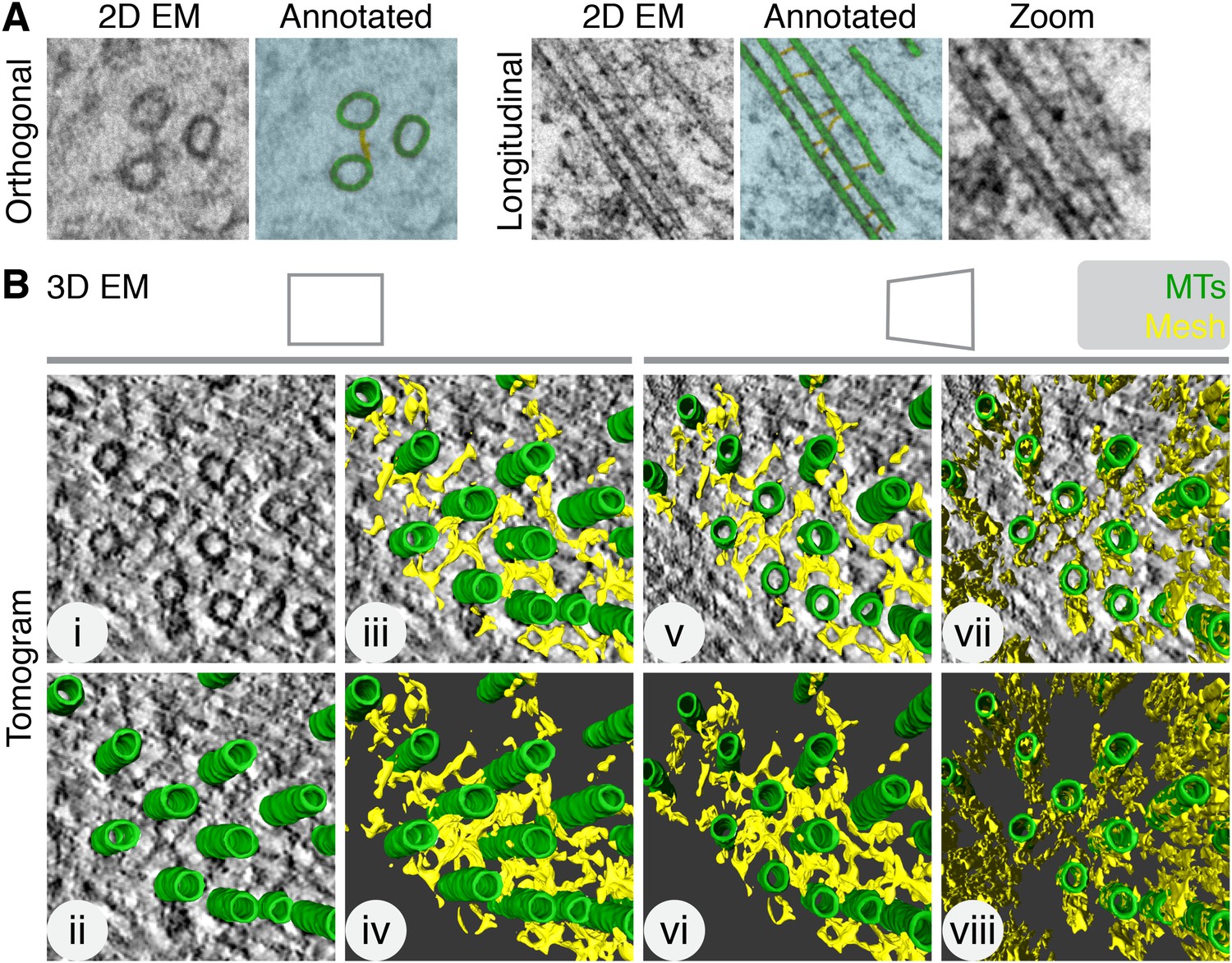
Intermicrotubule connectors in K-fibers are ‘bridges’ in 2D and a ‘mesh’ in 3D.
(A) 2D views of inter-MT bridges in sections taken orthogonally or longitudinally to the spindle axis. In the annotated version, MTs (green) and inter-MT bridges (yellow) are shown on a blue background. Zoom of longitudinal section is a 2× expansion of the lower part of the 2D EM view. (B) Orthoslice of a tomogram generated from a tilt series of a single section through a K-fiber preserved using HPF/FS (i). Overlaid is a hand-rendered 3D representation of MTs (green) (ii) and associated mesh (yellow) (iii). The model is shown alone (iv). For (v–viii), the tomogram is tilted to show the MT axis. In v and vi, the overlay and model are shown. In vii and viii, the same view is shown but with the mesh detected by the automated segmentation method. Note that sections taken >1 µm away from the kinetochore are shown in this and all subsequent figures. Tomogram thickness, 45.6 nm. For scale, MTs are 25 nm in diameter.
Figure 1—figure supplement 1
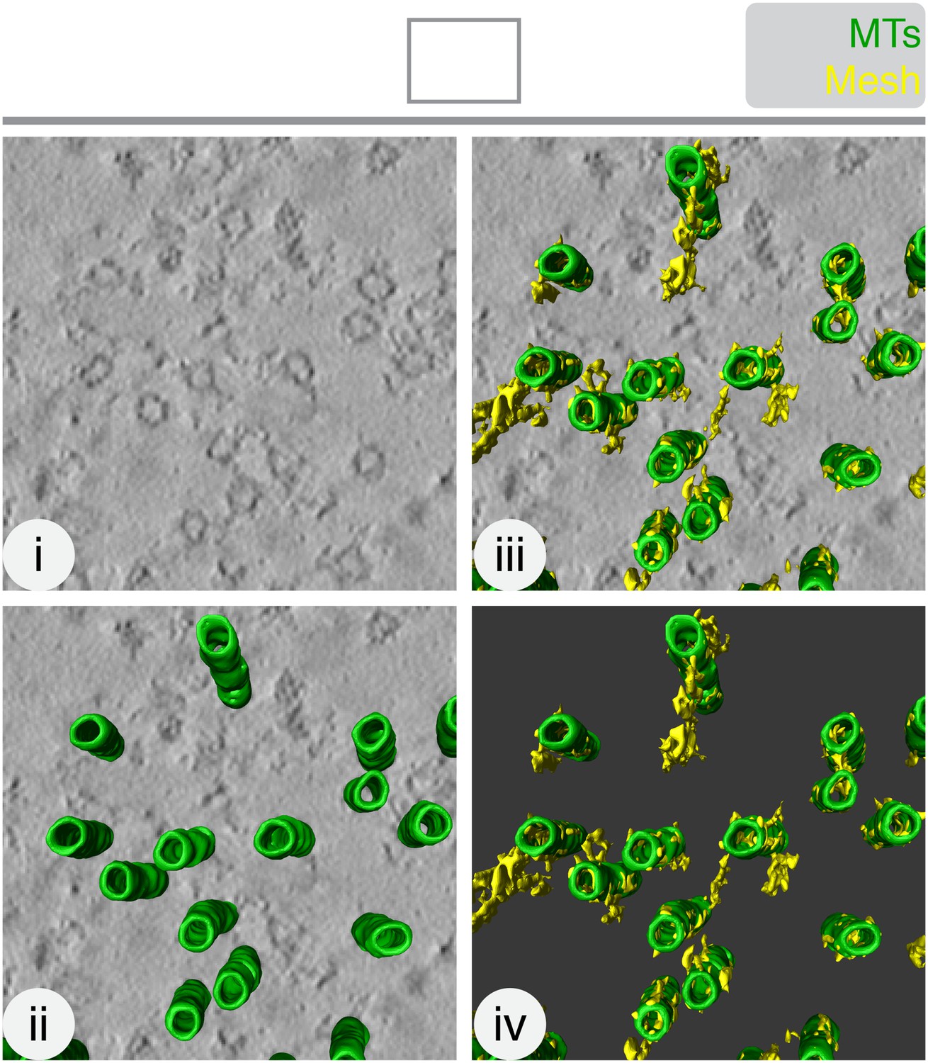
The mesh is visible, but not well preserved, in chemically-fixed K-fibers.
Orthoslice of a tomogram generated from a tilt series of a single section through a K-fiber fixed with glutaraldehyde (i). Overlaid is a hand-rendered 3D representation of MTs (green) (ii) and mesh segmented by automated detection (yellow) (iii). The model is shown alone (iv). Tomogram thickness, 51.3 nm. For scale, MTs are 25 nm in diameter.
Figure 1—figure supplement 2
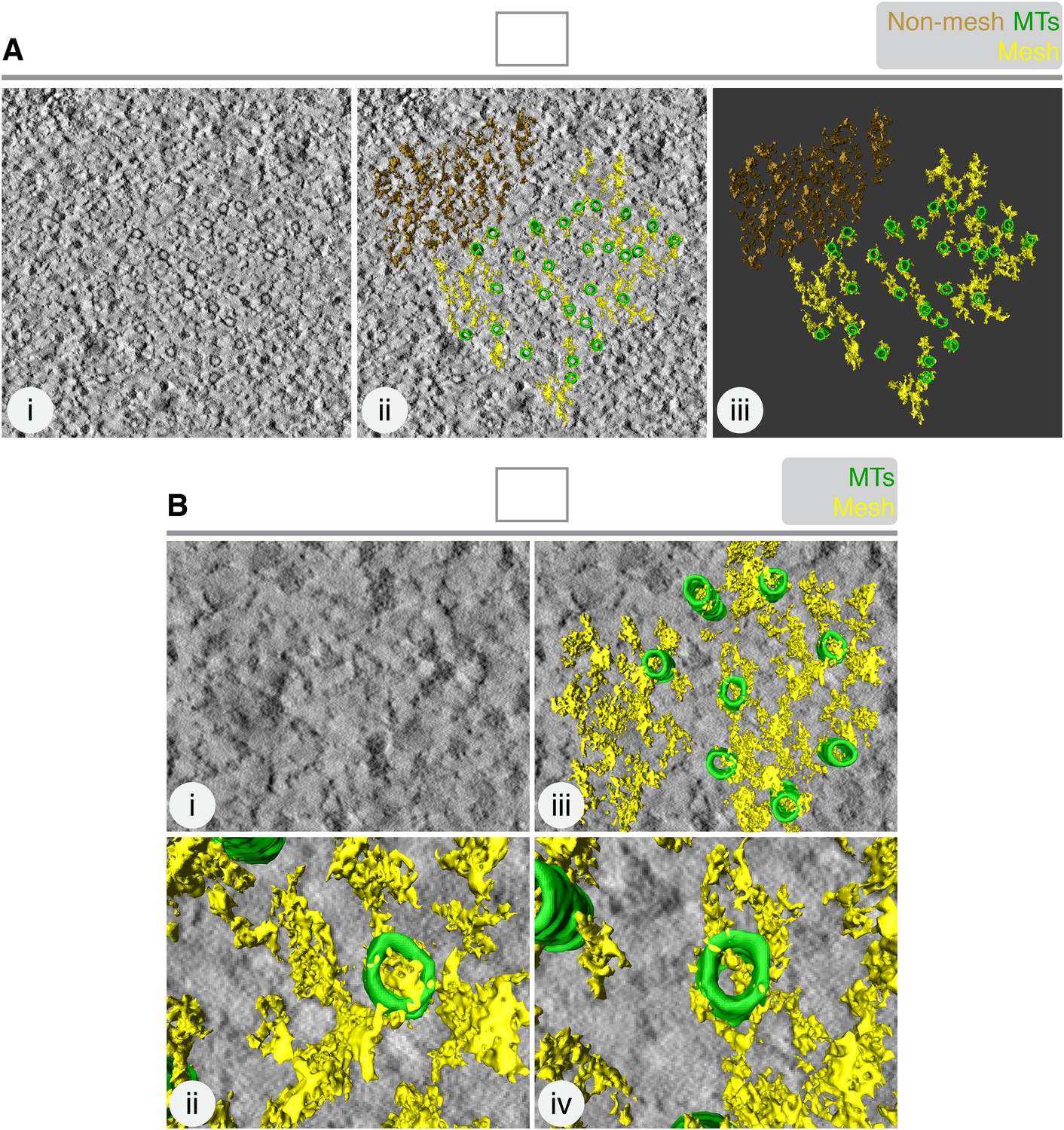
The mesh is associated with K-fiber MTs.
(A) 3D rendering of ‘non-mesh’ (brown) in a tomogram of a single K-fiber. Single orthoslice (i), with added rendering (MTs, green; mesh, yellow) (ii) and model alone (iii), is shown. Rendering the mesh involves segmenting density that is attached to the MTs. Here, density to the upper right of the K-fiber was rendered, although it was not touching MTs. The result is a particulate 3D structure that is dissimilar to the K-fiber mesh. (B) Translation of MT map from the tomogram in A, to the upper right corner. Mesh detection was performed as described in ‘Materials and methods’. Single orthoslice view (i), with added rendering (MTs, green; mesh, yellow) (ii). Zoomed views of two MTs and associated ‘pseudo-mesh’ are shown in (iii and iv). Note that the mesh passes through the MTs and is more particulate than the K-fiber mesh. Tomogram thickness, 35.2 nm.
Figure 2
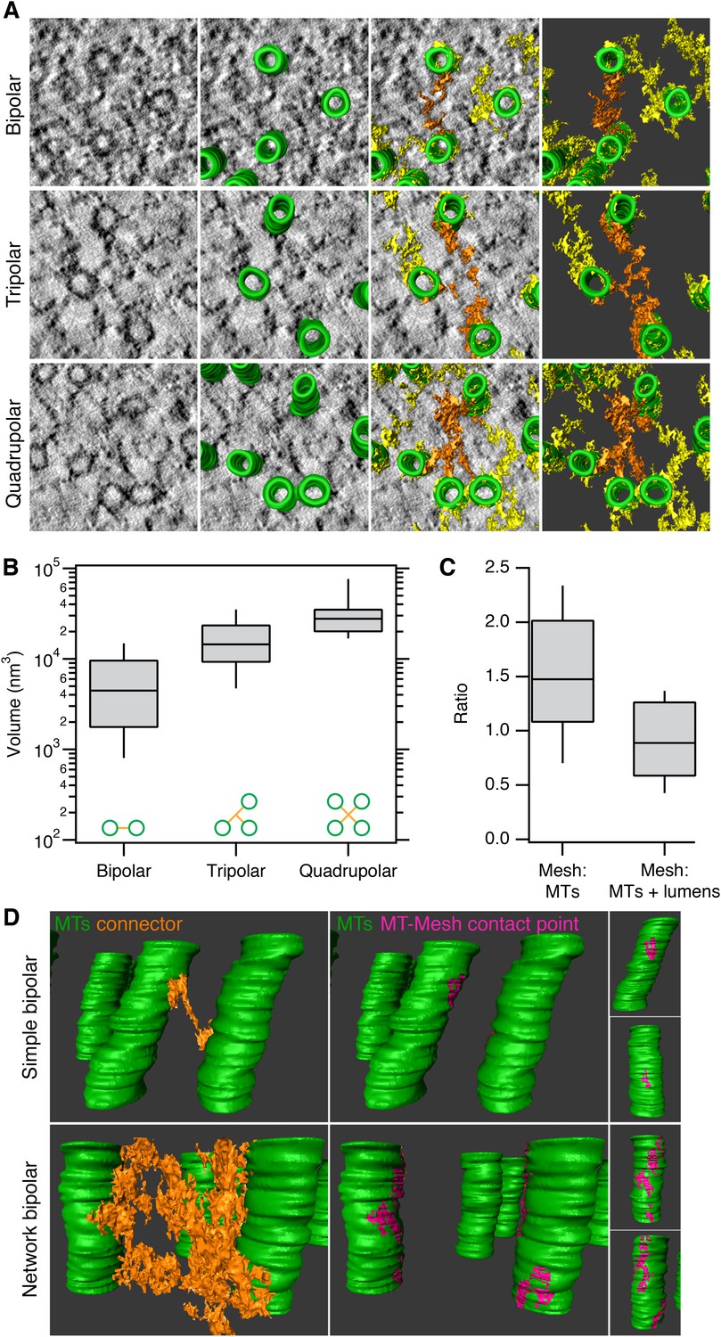
Inter-MT linkages are defined connectors with heterogeneous MT-mesh contacts.
(A) Examples of bipolar, tripolar, and quadrupolar connectors within the mesh. Single orthoslices from tomograms showing examples of different connectors. MTs are hand-rendered (green), mesh is automatically detected (yellow, see ‘Materials and methods’), and example connectors are highlighted orange. Tomogram thickness, 51.3 nm (bipolar) and 35.2 nm (tripolar and quadrupolar). (B) Box plots to show the volume of bipolar, tripolar, and quadrupolar connectors within the mesh from multiple tomograms. (C) Box plot to show the ratio of the volume of mesh relative to MTs (walls only) or MTs + lumens (‘filled-in’ MTs). Box plots show the median, 75th and 25th percentile, and whiskers show 90th and 10th percentile. (D) Heterogeneity of contacts between mesh and MTs. Two pairs of MTs are shown with a simple bipolar connector (above) or with a more complex connection (below). MTs (green) are shown with a single component of the mesh (orange). The contact points between the selected mesh and the MTs are shown in pink. Note the extensive mesh-MT contacts in the lower example. Tomogram thickness, 66.4 nm (simple) 64.8 nm (network). For scale, MTs are 25 nm in diameter.
Figure 3 with 1 supplement

Analysis of MT packing within a K-fiber.
(A) Box plots showing the number of MTs per K-fiber, the cross-sectional K-fiber area, and the density of MTs in the K-fiber. Nfiber = 26 (control), 37 (TACC3 OE). Box plots show the median, 75th and 25th percentile, and whiskers show 90th and 10th percentile. p values from Welch's t-test are shown. (B) Spatial maps of MTs (circles) in a representative K-fiber from a control (left) or TACC3 overexpressing cell (right) color-coded to show (i) the distance to the nearest neighbor or (ii) overlaid on a heatmap to show the number of MTs within 105 nm (center-to-center distance), 80 nm (edge-to-edge distance). (C) Histogram to show the frequency of distances to the nearest neighboring MT (i). A representation of the change in average (median) MT spacing to the nearest neighboring MT that is caused by TACC3 overexpression (ii). NMTs = 500–1324. (D) Analysis of tubulin intensity in the vicinity of kinetochores by confocal microscopy. Box plot to show the distribution of median values per cell of tubulin intensities in a sphere surrounding the kinetochore (i). Box plots show the median, 75th and 25th percentile, and whiskers show 90th and 10th percentile. p values from one-way Anova with Tukey's post hoc test are shown. Ncell = 20–25, Nkinetochore = 2823–3533. Schematic diagram of the changes in K-fibers induced by TACC3 overexpression (ii). K-fibers are thicker because MTs that are not stably attached to the kinetochore are recruited to the K-fiber bundle.
Figure 3—figure supplement 1
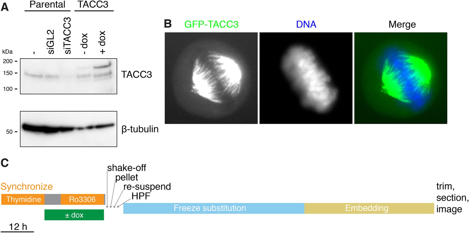
Inducible expression of GFP-TACC3 in HeLa cells to alter the composition of mesh.
(A) Western blot to show the extent of overexpression of TACC3 caused by inducing the expression of GFP-TACC3 in a stable TetOn HeLa cell line using 0.5 μg/ml doxycycline for 24 hr. The blot was probed for TACC3 and tubulin (as a loading control). (B) Widefield fluorescence micrographs of cells inducibly expressing GFP-TACC3. Note the strong fluorescence on K-fibers of the mitotic spindle. (C) Workflow to show the preparation of metaphase cells for analysis by 3D EM. Cells were synchronized and GFP-TACC3 expression was induced before release from RO3306 for 30–40 min. Mitotic cells were shaken off, pelleted, resuspended, and frozen under high pressure. Following freeze substitution and embedding, cells were trimmed and sectioned before imaging by electron microscopy. For details, see ‘Materials and methods’.
Figure 4 with 1 supplement
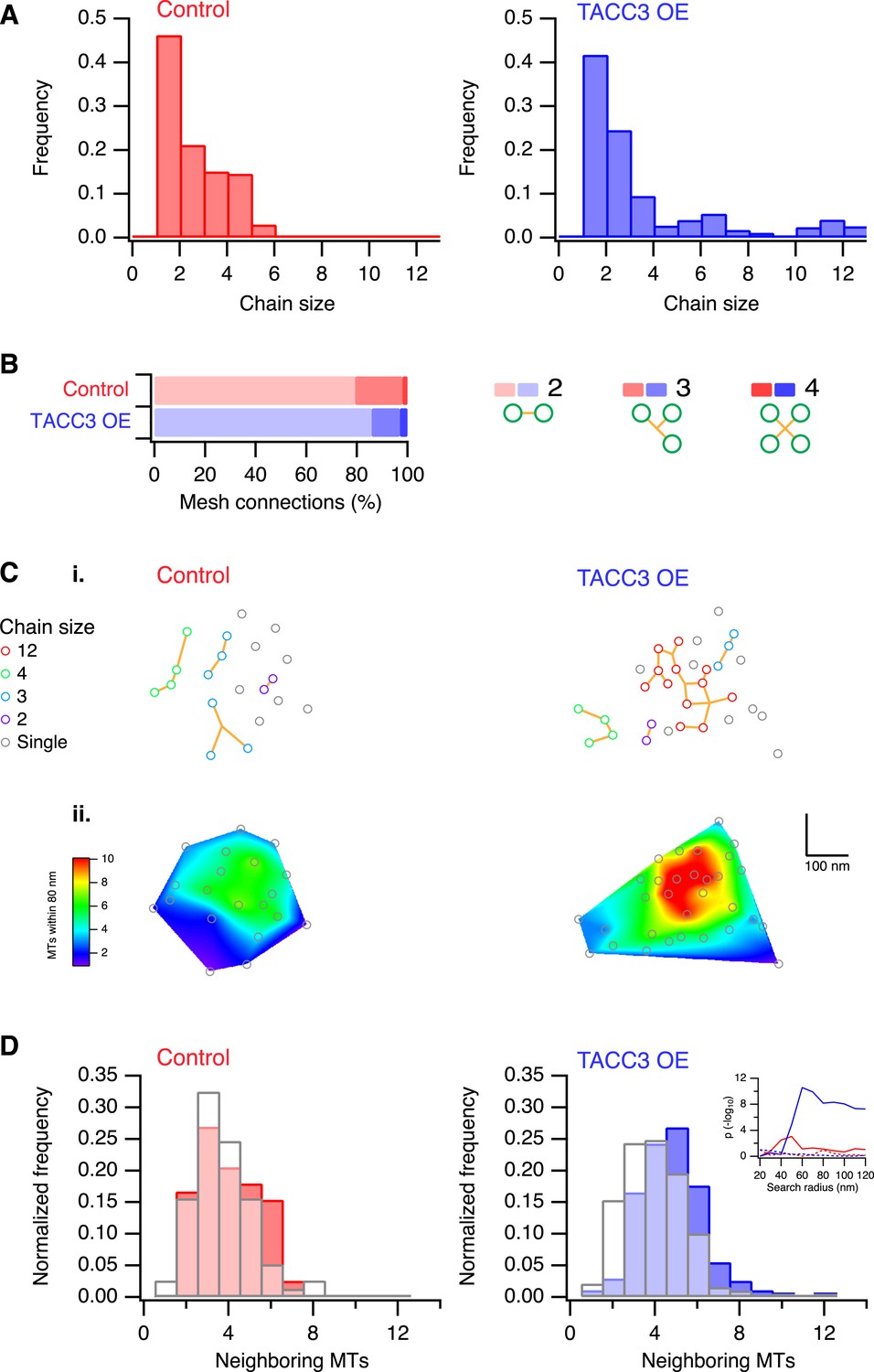
Analysis of MTs captured by mesh, their connectivity, and proximity.
(A) Histogram to show frequency of MT chain sizes detected in single section tomograms. MT chains are collections of MTs that are connected by mesh within a section. Note that single MTs do not feature. (B) Bar chart to show the proportion of mesh that is bipolar, tripolar, and tetrapolar, as a percentage of total mesh connections. (C) Analysis of MT connectivity and proximity. (i) Spatial maps of MTs (circles) in a representative K-fiber from a control (left) or TACC3 overexpressing cell (right). Chains of MTs are shown in color, gray circles show MTs that are not detectably connected to other MTs by mesh. Orange lines represent the mesh connections schematically (see Figure 4—figure supplement 1). (ii) Spatial maps are shown overlaid on heatmaps for the same fibers to show the number of MTs within 105 nm (center-to-center distance), 80 nm (edge-to-edge distance). Note that single (unchained) MTs are attached to the mesh, but that the MT to which they are attached is outside of the section. Tomogram thickness, 43.6 nm (Control), 28.8 nm (TACC3 OE). (D) Histogram to show frequency of MTs with a given number of neighboring MTs within 100 nm (center-to-center distance). MTs connected to others by mesh are shown in color, and single MTs are shown in white. Inset shows the p-value for comparisons calculated using search radii from 20 nm to 120 nm (center-to-center distance). Dotted lines show the same analysis following randomization of the chain membership data.
Figure 4—figure supplement 1

Examples of MTs chains and associated mesh.
Two example tomograms, which were annotated by 3D rendering and used to make the 2D maps illustrating MT position and chain membership in Figure 4C. MTs are colored as in Figure 4C, mesh associated with chained MTs is orange, other mesh is shown in yellow. Single orthoslice from the tomogram with rendered material is shown above, the MTs and mesh associated with chained MTs is shown below. Note that single (unchained) MTs are attached to the mesh, but that the MT/MTs to which they are attached are outside of the section. Tomogram thickness, 43.6 nm (Control), 28.8 nm (TACC3 OE). For scale, MTs are 25 nm in diameter.
Figure 5 with 2 supplements

Bundling of MTs in vitro by mesh components.
(A) Cartoon to illustrate two potential models for mesh function. In the passive model (left), MT distances are set by some other factor, and the mesh fills in the gaps to connect MTs. In the influential model (right), the mesh bundles MTs by favoring close spacing, this in turn influences MT spacing. (B) Representative fluorescence micrographs of rhodamine-labeled MTs incubated with the indicated proteins. Control (210 nM MBP-His6, 100 nM GST), PRC1 (2 µM His6-PRC1), and Mesh complex (10 nM MBP-ch-TOG-His6, 100 nM clathrin, 100 nM GST-TACC3-His6, 100 nM MBP-GTSE1-His6), all phosphorylated by TPX2(1–43)/Aurora-A. Scale bar, 10 µm. (C) Representative electron micrographs of MTs incubated with the indicated proteins as described in A. Pelleted material was chemically fixed, embedded in resin, sectioned, and imaged. Scale bar, 50 nm.
Figure 5—figure supplement 1

MT bundling using purified components.
Representative fluorescence micrographs of rhodamine-labeled MTs incubated with the indicated proteins. In all experiments, control was 210 nM MBP-His6 and 100 nM GST, and the total amount of protein was supplemented with MBP-His6 and GST to reach equimolarity. All samples were phosphorylated with Aurora A kinase and GST-TPX2(1–43). (A) MT bundling induced by higher concentrations of MBP-ch-TOG-His6, a range of 1–100 nM is shown. (B) Variability in MT bundling induced by higher concentrations of MBP-GTSE1-His6, a range of 1–100 nM is shown for two experiments. In one experiment, bundling is seen at 50 nM, and in another, no bundling is seen for concentrations up to 100 nM. (C) Combination of 10 nM MBP-ch-TOG-His6 with 1, 5, or 10 nM MBP-GTSE1 does not induce bundling. (D) Significant bundling observed with clathrin (100 nM), GST-TACC3-His6 (100 nM), MBP-ch-TOG (10 nM), and either 1, 5, or 10 nM MBP-GTSE1-His6. C and D were performed in parallel. Scale bar, 10 µm. (E) Coomassie blue-stained gels of purified protein components separated by SDS-PAGE. Molecular weights are indicated to the left.
Figure 5—figure supplement 2
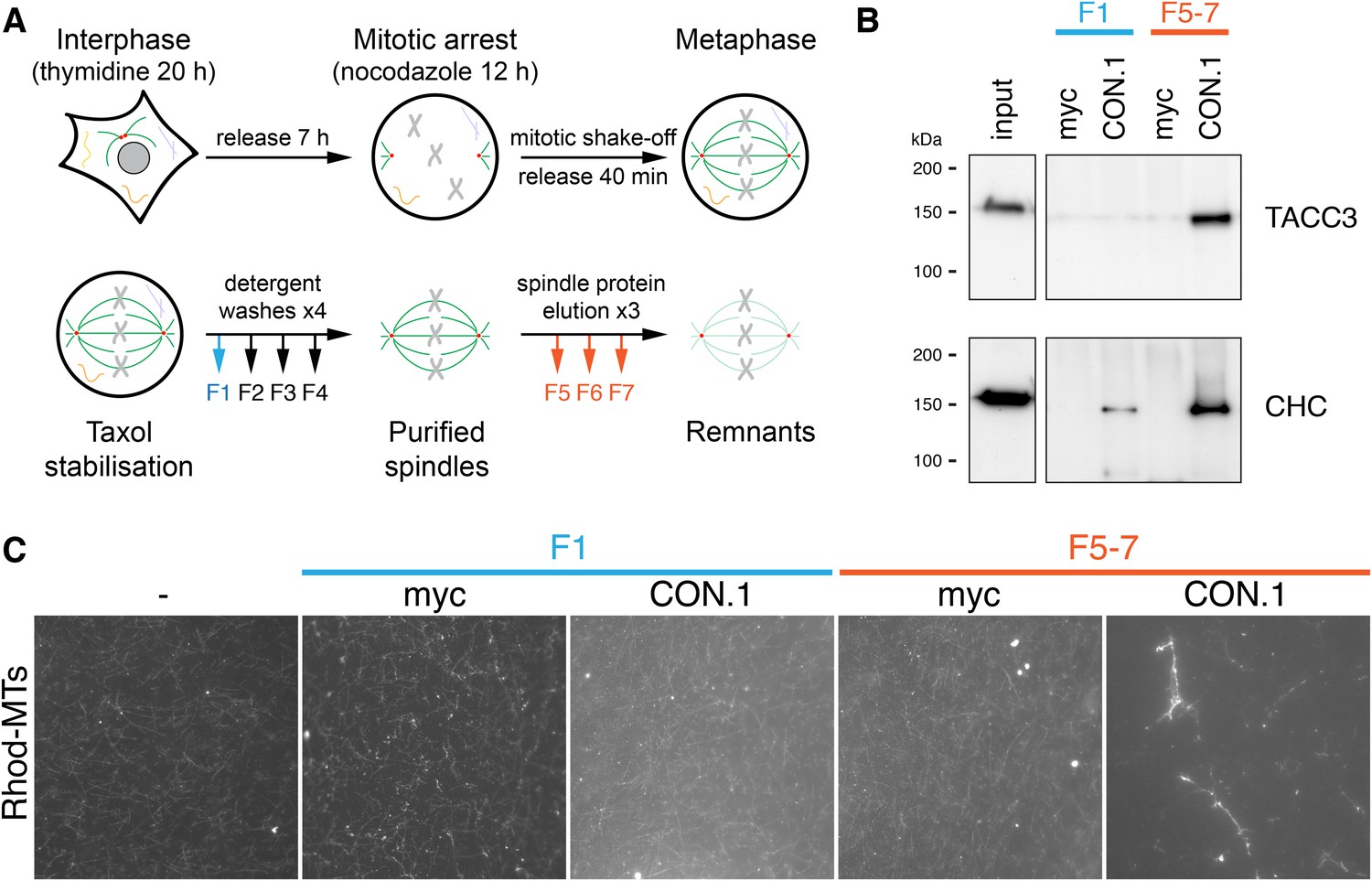
MT bundling using mesh complex immunoisolated from mitotic HeLa cells.
(A) Schematic diagram of the procedure to release mitotic spindle proteins from mitotic spindles at metaphase (described in Booth et al., 2011). (B) Western blot to show specific co-immunoprecipitation of TACC3/clathrin from spindle fractions (F5-7) but not from mitotic cytosol (F1) using an anti-clathrin light chain (CON.1). No immunoprecipitation of clathrin or TACC3 was seen with a control antibody (anti-myc). Western blots were probed with anti-TACC3 (rabbit polyclonal) or anti-clathrin heavy chain (CHC, TD.1). (C) Representative fluorescence micrographs of rhodamine-labeled MTs incubated with beads from the immunoprecipitation shown in B. Significant bundling was seen for clathrin IPs from F5-7 only. No bundling activity was seen with control IPs or clathrin IPs from F1. Beads are out of frame for clarity. Scale bar, 10 µm.
Figure 6
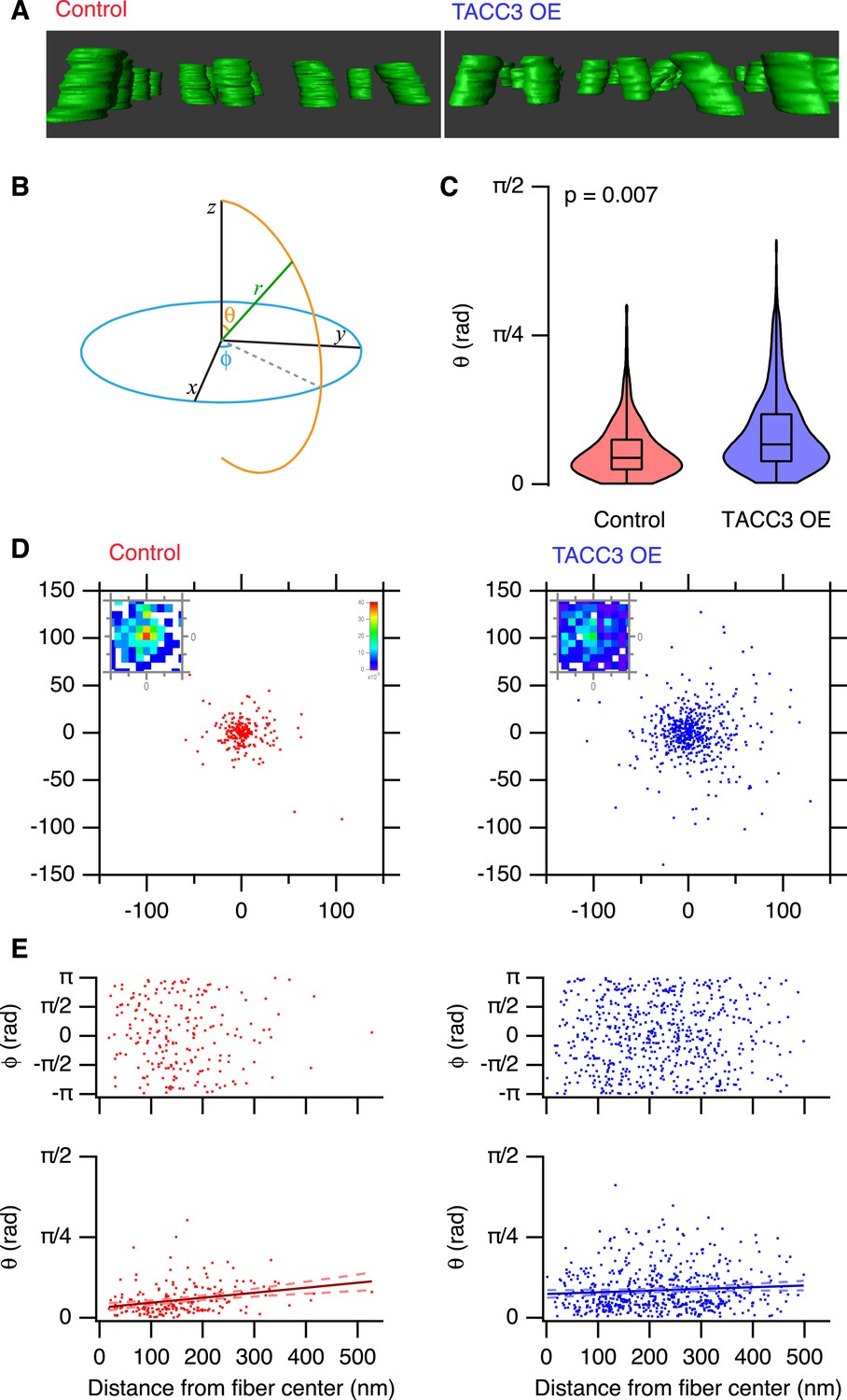
Analysis of MT trajectories within a K-fiber.
(A) Representative ‘side views’ of rendered MTs in single tomograms of individual K-fibers from control (left, red, Video 2) or TACC3 OE (right, blue, Video 3) cells. Tomogram thickness, 66.4 nm (Control) trimmed to 34.2 nm, 34.2 nm (TACC3 OE). For scale, MTs are 25 nm in diameter. (B) Aide memoire of the spherical coordinate system. Trajectories of MTs (green line) in K-fibers were defined and normalized via Euler's rotation (see ‘Materials and methods’) such that the overall trajectory of all fibers pointed to the zenith. Measurements of polar angle (θ) and azimuthal angle (φ) were made from the normalized sets and are presented in C–E. (C) Violin plots of the polar angles for MTs in K-fibers from control and TACC3 overexpressing cells. Box plots show the median, 75th and 25th percentile, and whiskers show the minimum and maximum. Violins show a kernel density estimate of the data and are trimmed to the minima and maxima. Comparison of the median MT angle from each K-fiber, Wilcoxon Rank Sum Test, p = 0.007, Nfiber = 12–15. (D) Illustration of the deviation of MTs from the fiber axis caused by TACC3 overexpression. Cartesian coordinates of the intersection of individual MT vectors that start from a common origin (0, 0, 0), with an x-y plane at z = 100 nm. To account for the difference in number of MTs, the insets show a normalized 2D histogram of these coordinates cropped to a 40 × 40 nm square centered at 0, 0, 100. (E) Plots of azimuthal angle (above) and polar angle (below) as a function of distance from the fiber center (defined as described in the ‘Materials and methods’). Line of best fit is shown with 95% confidence bands (dashed line), r2 = 0.07 (control), and 0.007 (TACC3 overexpression).
Figure 7 with 1 supplement

Mitotic consequences of TACC3 overexpression.
(A) Cartoon representation of the stages of mitosis captured in live-cell imaging experiments. Cells expressing H2B-mCherry were staged as indicated with the transition to prometaphase marked by nuclear envelope breakdown; transition to metaphase marked by alignment of the last chromosome to the metaphase plate; to anaphase marked by first sign of chromosome segregation and transition to telophase marked by decondensation of H2B-mCherry. These events allowed us to assign prometaphase-to-metaphase (PM-M, dark green), metaphase-to-anaphase (M-A, light green), and anaphase-to-telophase (A-T, light blue). (B) Mitotic stage duration for individual cells. Time taken to go from prometaphase-to-metaphase (PM-M), metaphase-to-anaphase (M-A), or anaphase-to-telophase (A-T) is shown for control (red, above) or GFP-TACC3 overexpressing (blue, below) cells expressing H2B-mCherry. Each line represents a single cell. The time when the last chromosome aligned was set as 0 (metaphase). Cells that did not achieve metaphase halt at 0. Note that the time axis is truncated to show a 4 hr window centered on metaphase. Ncell = 163–169, Nexp = 4. (C) Still images of example cells from live-cell imaging experiments to determine mitotic progression. Detection of H2B-mCherry is shown on an inverted grayscale. Time in min is shown and the colored bars represent the staging, as in A and B. (D) Box plots to summarize mitotic progression experiments. Time taken to go from prometaphase-to-metaphase (PM-M), metaphase-to-anaphase (M-A), or anaphase-to-telophase (A-T) is shown for control (red) or GFP-TACC3 overexpressing (blue) cells. Whiskers show 90th and 10th percentiles.
Figure 7—figure supplement 1
Mitotic consequences of TACC3 depletion.
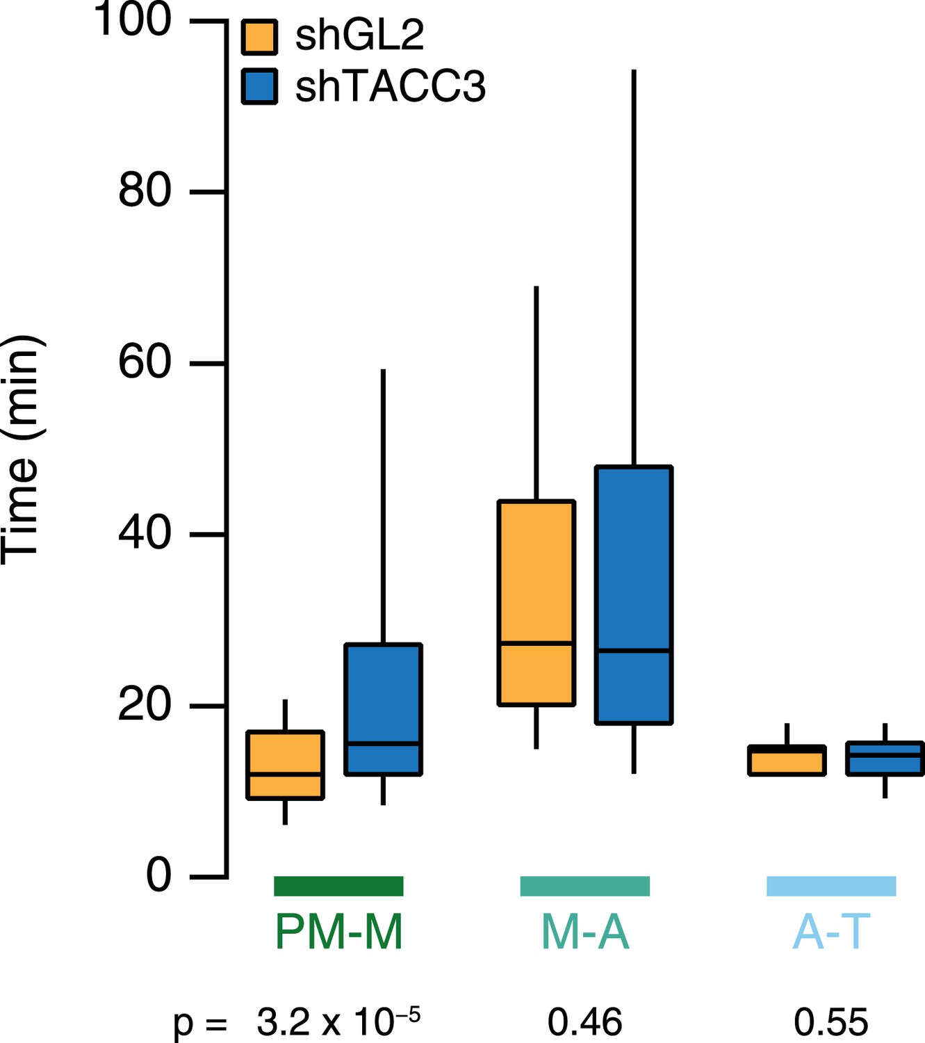
Box plots to summarize mitotic progression experiments. Time taken to go from prometaphase-to-metaphase (PM-M), metaphase-to-anaphase (M-A), or anaphase-to-telophase (A-T) is shown for control (orange) or TACC3-depleted (blue) HeLa cells using shRNA-mediated knockdown. Whiskers show 90th and 10th percentiles. Ncell = 122–138, Nexp = 2.
Author response image 1
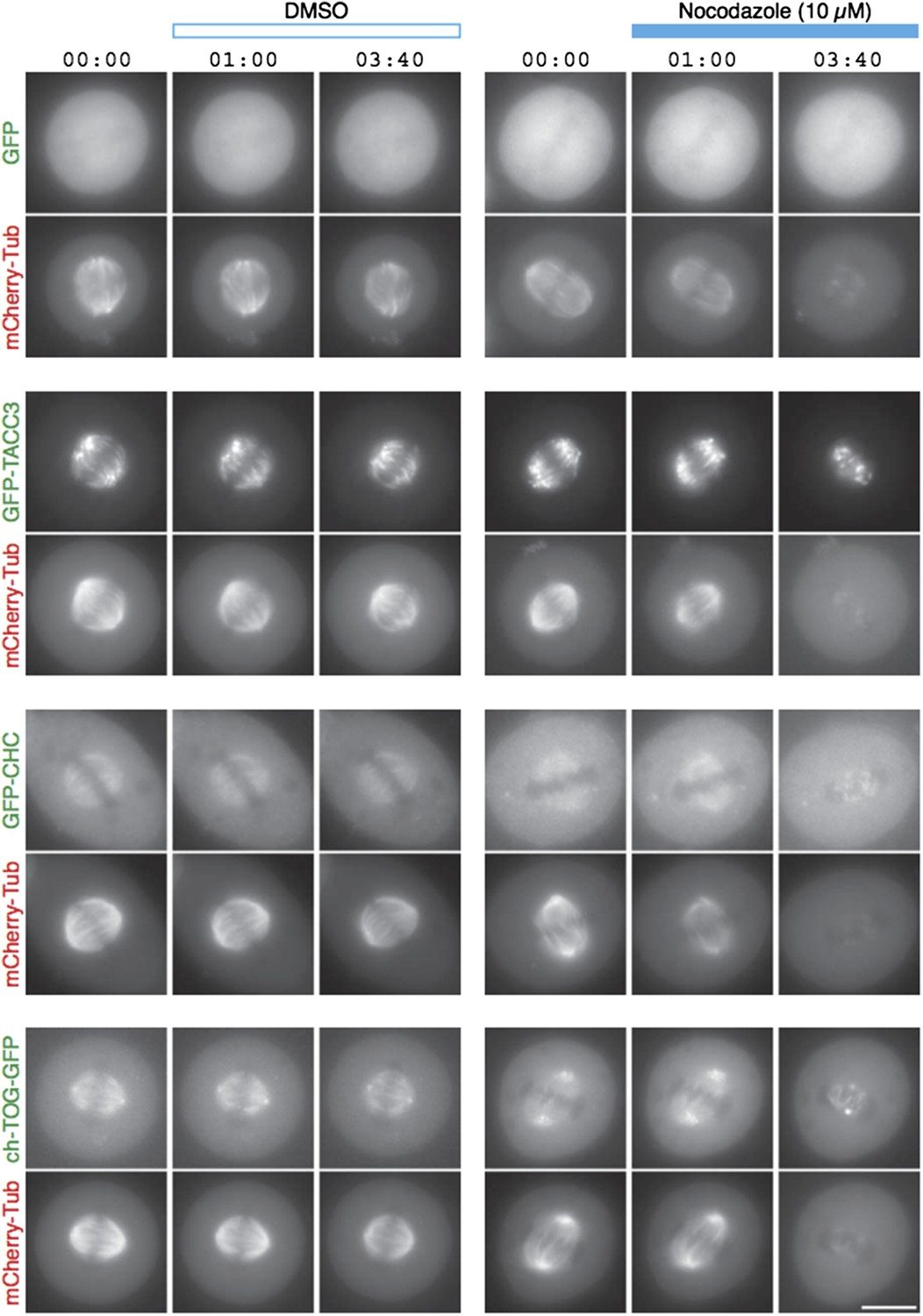
TACC3 mesh complex does not persist in a “spindle matrix” after depolymerization of MTs.
Still images from live-cell imaging experiments to visualize metaphase HeLa cells expressing mCherry-tubulin and the indicated GFP-tagged protein. Cells were exposed to DMSO (control, left) or nocodazole (10 µM, right) after 1 min. MT depolymerization, monitored by mCherry-tubulin, caused mislocalization of clathrin and ch-TOG. When over-expressed, GFP-TACC3 forms aggregates in the absence of MTs.
Author response image 2
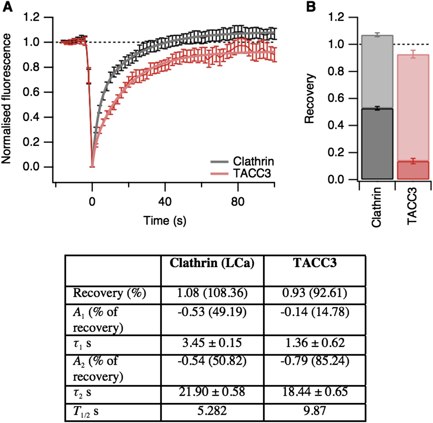
Fluorescence recovery after photobleaching (FRAP) analysis of TACC3 dynamics in mitotic cells.
(A) Average FRAP traces for metaphase cells expressing GFP-tubulin and either mCherry-clathin light chain a or mCherry-TACC3. Plots show the mean ± s.e.m. fluorescence that is scaled to examine the recovery following photobleaching. N = 10 cells. Recovery was best fit by a double exponential function (thick line). (B) Stacked bar chart to show the proportion of recovery by fast (dark) and slow (light) processes. The bar indicates the scaled co-efficient, error bars are ± S.D. of the fitting procedure. Kinetic parameters for the fits are shown below.
Videos
Video 1
Example of the K-fiber mesh from a normal HeLa cell at metaphase.
Tomogram of a K-fiber. The mesh (yellow) is shown by manual rendering and by automated rendering. MTs (green) were rendered by hand. All segmentation was smoothed in Amira.
Video 2
Example of MT organization in a K-fiber from a control cell.
Tomogram of a K-fiber. MTs (green) were rendered by hand. All segmentation was smoothed in Amira.
Video 3
Example of MT organization in a K-fiber from a GFP-TACC3 expressing cell.
Tomogram of a K-fiber. MTs (green) were rendered by hand. Pale green is used to highlight two highly deviant MTs. All segmentation was smoothed in Amira.
Additional files
-
Source code 1
Custom written code in IgorPro 6.36 (Wavemetrics) was used for all analysis and plotting.
- https://doi.org/10.7554/eLife.07635.020
Download links
A two-part list of links to download the article, or parts of the article, in various formats.
Downloads (link to download the article as PDF)
Open citations (links to open the citations from this article in various online reference manager services)
Cite this article (links to download the citations from this article in formats compatible with various reference manager tools)
The mesh is a network of microtubule connectors that stabilizes individual kinetochore fibers of the mitotic spindle
eLife 4:e07635.
https://doi.org/10.7554/eLife.07635


