Temporal structure in associative retrieval
- University College London, United Kingdom
Figures
Figure 1

Task design and behavior.
Subjects participated in a sensory preconditioning task comprising three phases: Association, Reward and Decision. (A) In the Association phase, subjects were exposed to pairs of stimuli (presented sequentially). One member (called Si) of each pair was taken from one of three classes (faces, bodies, and scenes); the other member (Sd) was a fractal. In the Reward phase, some of the fractals (labelled Sd+) were paired with reward; the others (labelled Sd−) were not. Through the pairing, this implicitly established a separation between Si+ and Si−. In the Decision phase, subjects chose between Si+ and Si− within the same category, or between Sd+ and Sd−. All photos shown are from pixabay.com and are in the public domain. (B) In the Decision phase, subjects displayed a strong preference for Sd+ over Sd− (p = 6.9 × 10⁻⁴, one-sample t-test). There was no preference at the group level for Si+ over Si−, but we exploited the variability between subjects for value-related analyses. The change in relative liking from before to after the experiment was more positive for Sd+ than Sd− (p = 0.04, one-sample t-test); but there was no significant difference between the changes for Si+ and Si−. Bar heights show group means and dots show individual subjects. Error bars show standard error of the mean.
Figure 2

Event-related field (ERF) discriminates between categories (face/body/scene) at time of Si presentation.
Sensors became category-discriminative in two waves. (A) The first time, relative to stimulus onset, when the relationship between ERF amplitude and category membership became significant by ANOVA (significance threshold set at 95% of peak-level (across all sensors and all time) log10(p) of 100 shuffles) at each of 275 sensors. Many occipital and temporal sensors first became predictive of Si category between 90 and 230 ms post stimulus onset, followed by some parietal and frontal sensors ranging from 330–550 ms post stimulus onset. Open circles indicate the sensors that never reached 95% peak-level. (B) Histogram of how many sensors first became significantly discriminative at each time following stimulus presentation.
Figure 3 with 6 supplements
Multivariate analysis reveals two temporal components of evoked response to visual stimuli.
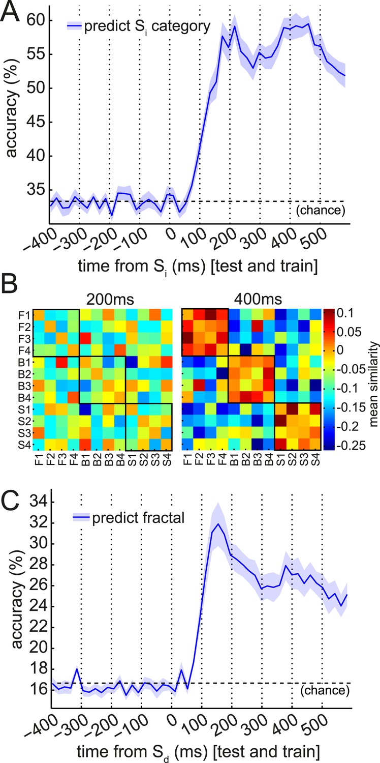
(A) Multivariate decoding performed well to predict the category of photograph (Si) in the Association phase. Cross-validated linear SVM prediction accuracy using all 275 sensors at each time bin is shown. A pattern of two distinct peaks in classifier accuracy around 200 ms and 400 ms after Si onset is evident. (B) At 200 ms after Si onset, there was no difference in representational similarity between same-category and different-category Si objects (left panel, p = 0.2 by t-test between subjects). At 400 ms, representational similarity was higher for same-category than different-category objects (right panel, p = 5 × 10⁻⁷). F1–F4, B1–B4 and S1–S4 refer to the unique faces, bodies and scenes presented during the Association phase. (C) When discriminating fractal identity (i.e., a 6-way classification problem of stimuli with no natural categories), performance was sharply peaked before 200 ms after fractal onset. Shaded area shows standard error of the mean.
Figure 3—figure supplement 1
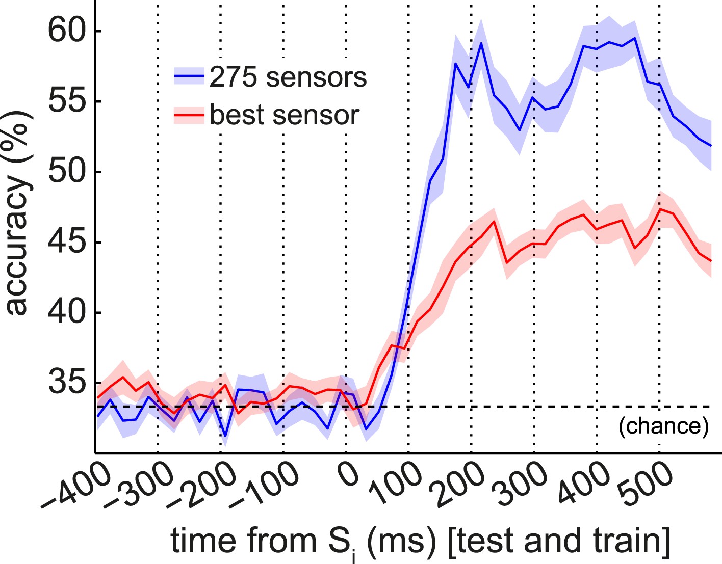
Univariate classification using best sensor.
We tested the capacity of the most discriminative single sensor (selected separately for each subject) to predict the Si category, using linear support vector machines (SVM) with a single feature. The accuracy of this univariate classifier peaked at 47.4 ± 1.3% in cross-validation (red trace). (When using a nearest-mean univariate classifier rather than a univariate SVM, accuracy peaked at 45.6 ± 1.9%.) We constructed independent null distributions at each time bin by repeating this procedure 100 times with randomly shuffled category labels. At 200 ms post-stimulus, the median of the null distribution was 37.0% accuracy (greater than 1/3rd due to allowing the best sensor for each subject), while the 95th percentile of the null distribution was 38.6%. Blue line shown is multivariate SVM performance, from Figure 3A, for comparison.
Figure 3—figure supplement 2
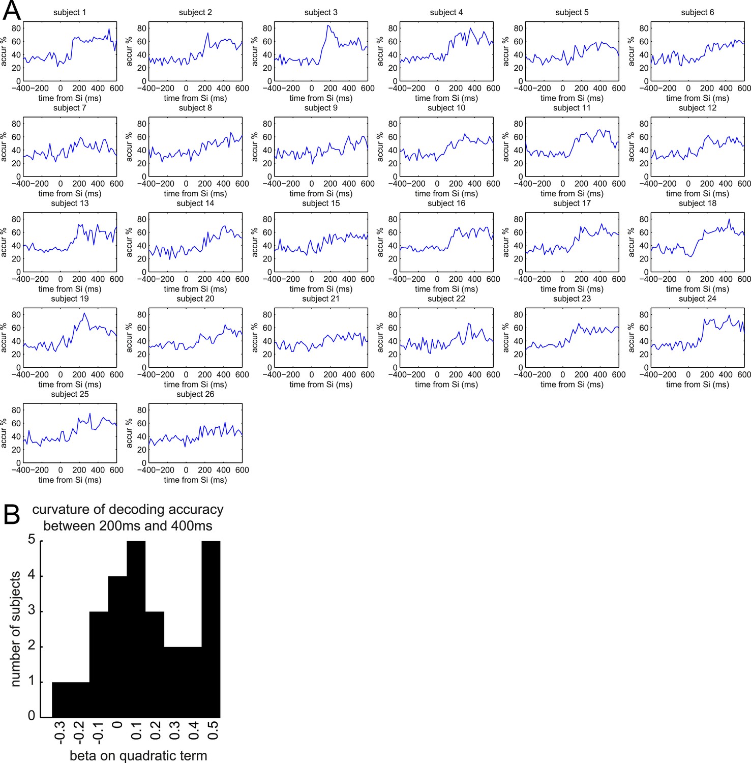
Multivariate classification of Si for individual subjects.
(A) Classification accuracy in predicting Si category in Association phase for individual subjects. (B) We fit regression models to each subject's accuracy curve (between 200 ms and 400 ms), with constant, linear, and quadratic terms. This histogram shows the estimated betas on the quadratic term. Positive beta indicates positive curvature of the accuracy curve between 200 ms and 400 ms. No individual subject reached Bonferroni-corrected significant betas on the quadratic term of the regression.
Figure 3—figure supplement 3
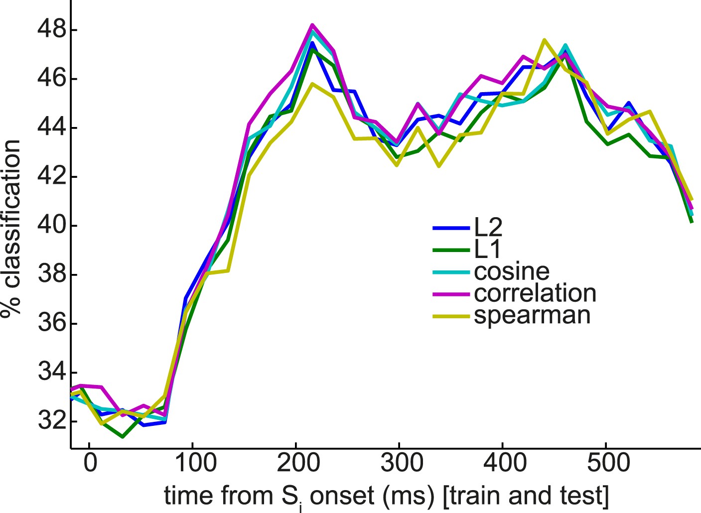
Nearest-mean multivariate classifiers, under a variety of distance metrics, underperform SVM but extract a similar pattern of multiple peaks in classification performance.
Compare to SVM applied to the same classification problem in Figure 3B, blue trace.
Figure 3—figure supplement 4
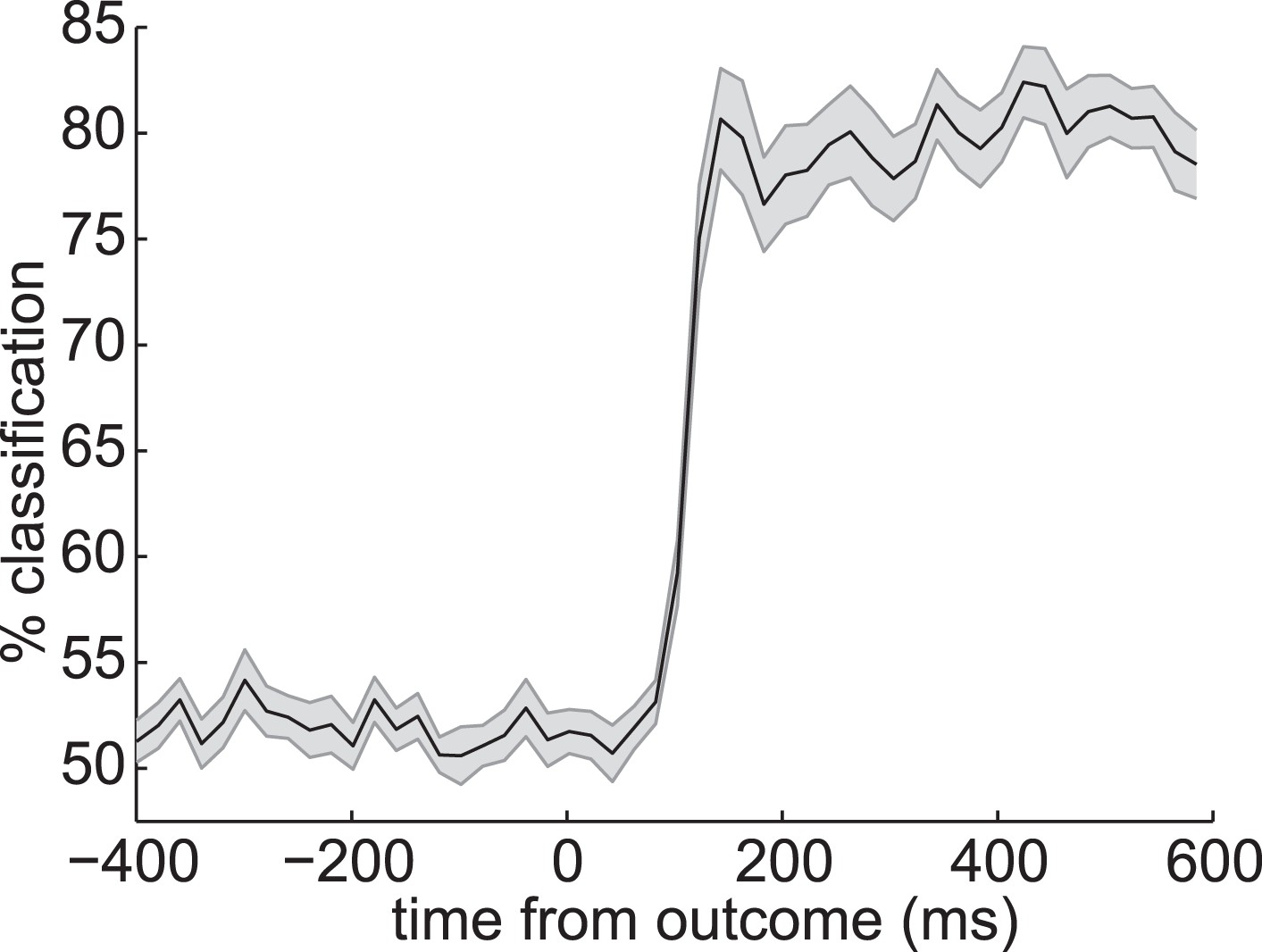
Decoding outcome identity.
At the time of outcome, there was a strong neural representation of the identity of the outcome itself (the coin or blue square). Together with Figure 3D, this suggests that the neural signal at time of Sd and outcome strongly encoded a representation of the on-screen stimulus.
Figure 3—figure supplement 5
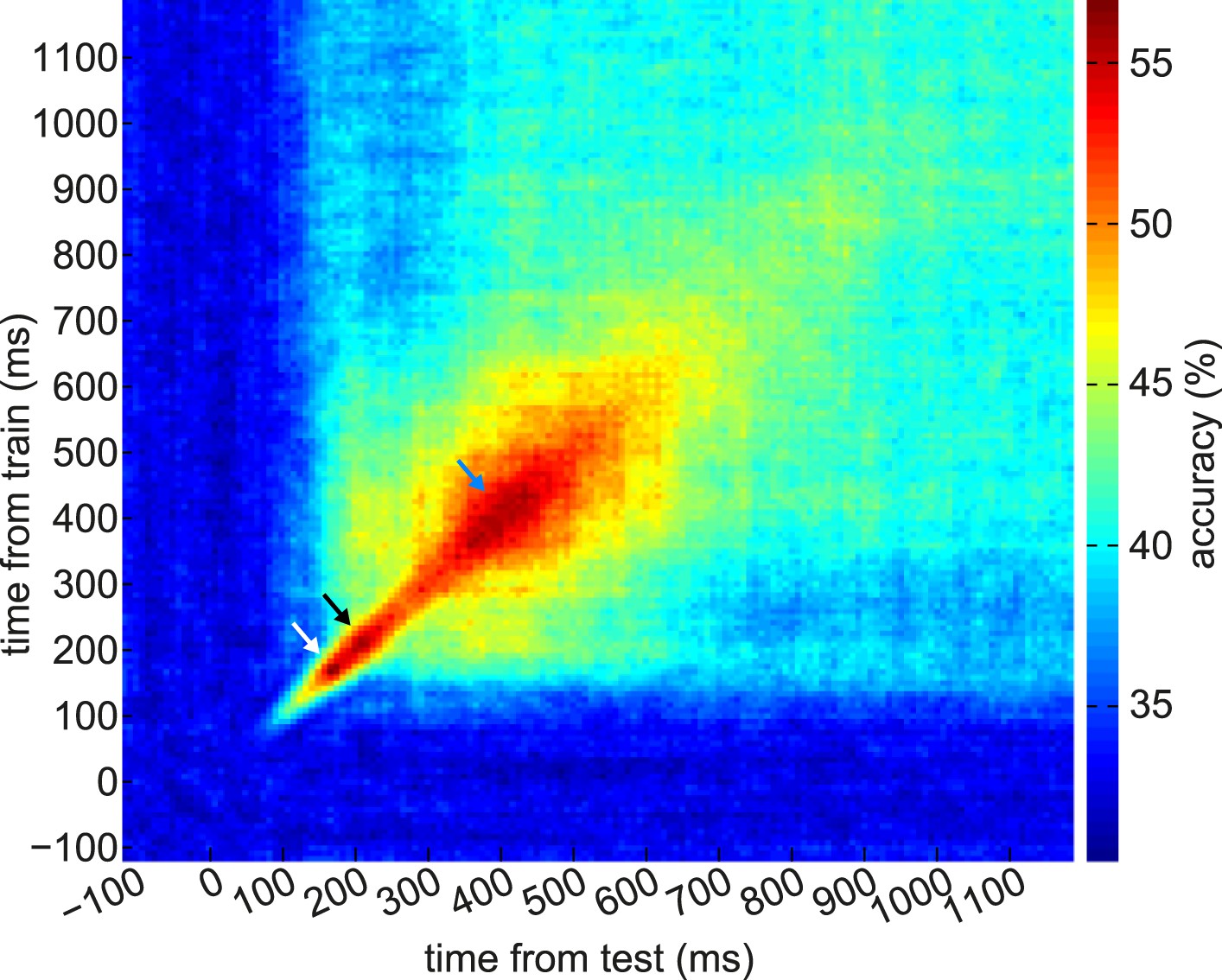
Generalization of instantaneous representational patterns over time, with finer temporal binning.
Here we trained classifiers on every time bin relative to the onset of Si in the Association phase, and tested at every time bin relative to the same onsets. For this figure we binned the data into 8 ms bins rather than the 20 ms bins used in the rest of the paper. Each cell of this grid shows cross-validated prediction accuracy, so the diagonal is equivalent to Figure 3B, blue trace (except that this figure has finer temporal binning). Later classifiers generalized better over time than earlier classifiers. We note the possibility that the 200 ms peak of classification might be decomposed into further sub-peaks (white and black arrows); however, we were unable to statistically separate these sub-peaks, due to variability between subjects. The peak at 400 ms is evident (blue arrow). Absolute classification accuracy is lower than with more coarsely binned data, likely due to a poorer signal to noise ratio.
Figure 3—figure supplement 6
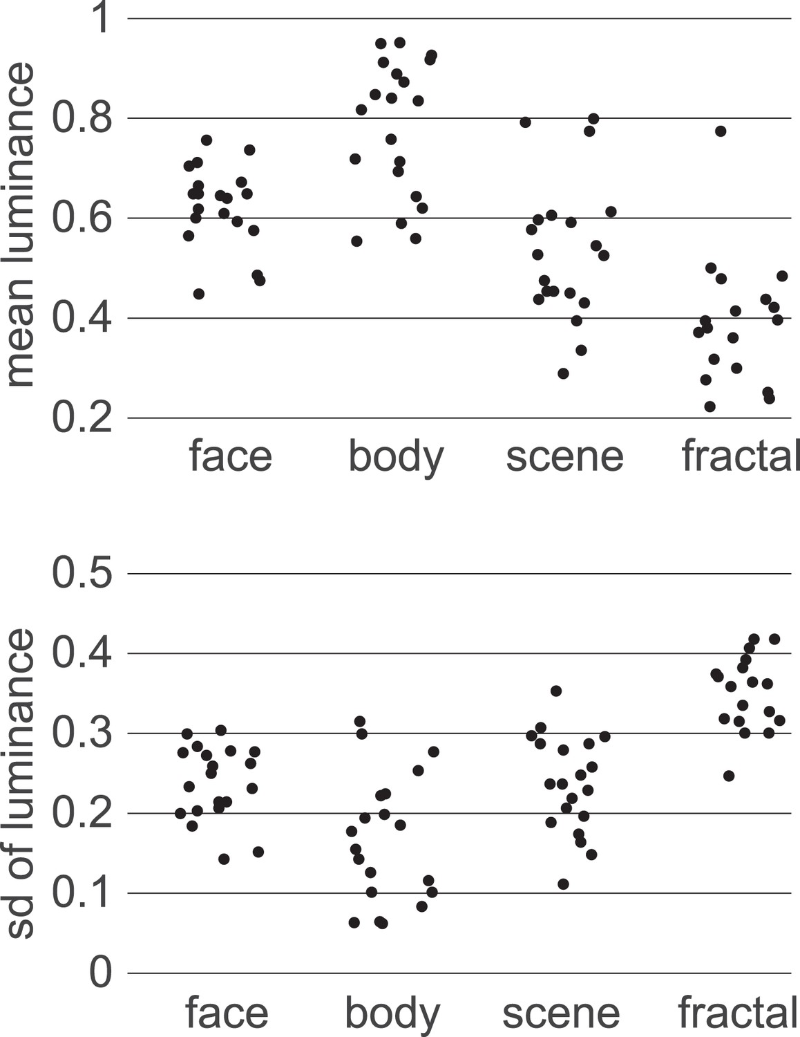
Image statistics.
Image types varied in low-level visual properties as well as shape. The methods we used are agnostic as to the kinds of features that drove the neural representation of category.
Figure 4
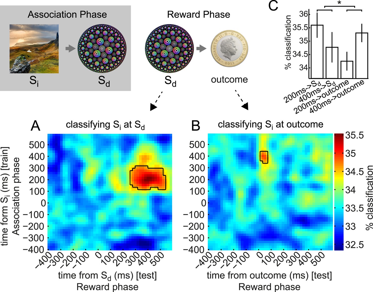
Early and late components of associated object representation retrieved at time of cue and outcome, respectively.
During the Reward phase, the 200 ms component of the Si representation was retrieved for an extended period from shortly after Sd was presented, while the 400 ms component of Si representation was retrieved around the time the outcome was presented. (A) Classifiers trained around 200 ms after Si presentation in Association phase and tested around 400 ms after Sd presentation in Reward phase decode the object category previously associated with the Sd. Photo is from pixabay.com and is in the public domain. (B) Classifiers trained around 400 ms after Si presentation and tested 70 ms after outcome presentation decode the object category previously associated with the Sd. In A and B, black outlines show p = 0.05 peak-level significance thresholds (empirical null distribution generated by 1000 random permutations of training category labels, see Methods for more details). (C) Peak classification accuracy in the 200 ms and 400 ms rows of A and B. By 2-way ANOVA, there was no main effect of 200 ms vs 400 ms or of Sd vs outcome, but there was a significant interaction (p = 0.04). Error bars show standard error of the mean.
Figure 5
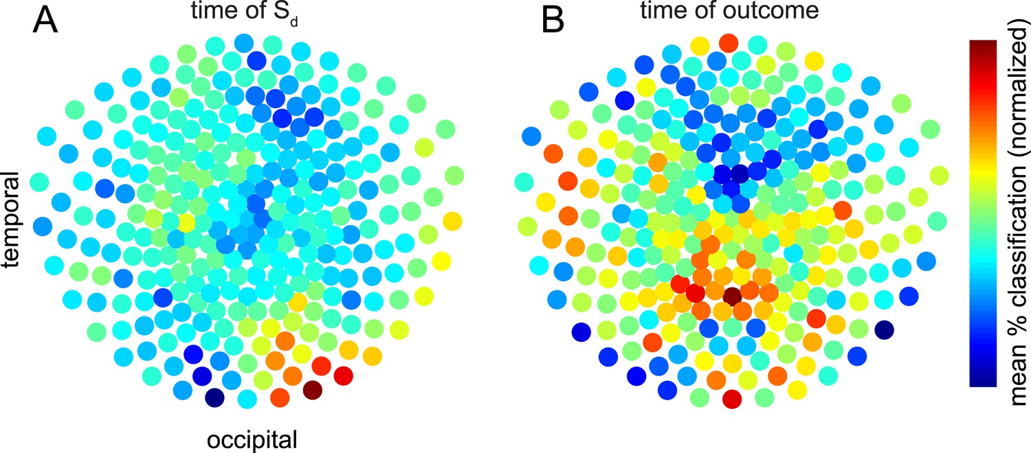
Contributions of sensors to retrieval.
To explore which brain areas carried the information about Si that was retrieved at the time of Sd and outcome, we copied the procedure of training linear category classifiers on presentation of Si, and predicting the category at the time of Sd or outcome—but instead of using all 275 sensors, we repeated the analysis 2000 times using subsets of 50 sensors randomly selected on each iteration. The contribution of sensor s was taken to be the mean of all prediction accuracies (within 60 × 60 ms temporal ROIs containing the peak time bins) achieved using an ensemble of 50 sensors that included s. Intriguingly, the information about the category of Si retrieved at the time Sd was presented emerged primarily from occipital sensors (A), while the information about the category of Si retrieved at the time the outcome was shown appeared more strongly in parietal and temporal sensors (B). In the difference between the two conditions, no individual sensor survived correction for multiple comparisons. However, a linear SVM was reliably able to classify whether a spatial pattern belonged to Sd or outcome (71.2% accuracy, p = 0.002 by one-sided binomial test against chance classification).
Figure 6
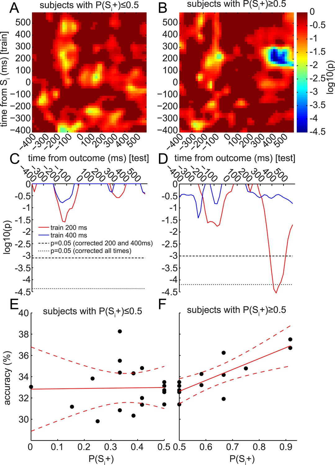
Retrieval of early component of Si representation predicts value updating across subjects.
At the group level, only the 400 ms component was significantly retrieved at the time of outcome (cf. Figure 4B). However, at the single-subject level, the degree of retrieval of the 200 ms component correlated with value updating. As in Figure 4B, the accuracy of classifiers trained at each time bin around Si (in the Association phase) was tested at each time bin around the time of outcome (in the Reward phase) to predict the category of the Si associated with the Sd preceding the outcome. In each time*time bin, this accuracy was regressed, across subjects, against the behavioral preference for Si+ over Si− from the Decision phase (i.e., P(Si+)). As we only explored positive correlations, one-tailed log10 p-values of the regression are reported. (A) In subjects who preferred Si− over Si+, there were no correlations between the degree of preference and the degree of reinstatement of Si at outcome. (B) In subjects who preferred Si+ over Si−, there was a strong correlation between the degree of preference and the degree of reinstatement. This correlation peaked at around 400 ms after outcome onset. (C, D) Red and blue traces show single rows of panels A and B at 200 and 400 ms. Significance was tested by randomly shuffling subject identities to obtain a null distribution of peak-level log10 p-values. Thresholds are shown at 95% of the null distribution of the peak-level of 200 and 400 ms rows, and at 95% of the null distribution of peak-level of all rows. (E, F) Raw classification accuracies underlying the correlations in A–D, when training at 200 ms after Si onset and testing at 400 ms after outcome onset. Each point is a subject.
Download links
A two-part list of links to download the article, or parts of the article, in various formats.
Downloads (link to download the article as PDF)
Open citations (links to open the citations from this article in various online reference manager services)
Cite this article (links to download the citations from this article in formats compatible with various reference manager tools)
Temporal structure in associative retrieval
eLife 4:e04919.
https://doi.org/10.7554/eLife.04919


