Evolutionary genomics of epidemic visceral leishmaniasis in the Indian subcontinent
- Institute of Tropical Medicine, Belgium
- Wellcome Trust Sanger Institute, United Kingdom
- National University of Ireland Galway, Ireland
- BP Koirala Institute of Health Sciences, Nepal
- Banaras Hindu University, India
- University of Western Australia, Australia
- Charité Universitätsmedizin Berlin, Germany
- University of Glasgow, United Kingdom
- Northeastern University, United States
- Université Libre de Bruxelles, Belgium
- Indian Institute of Chemical Biology, India
- University of Antwerp, Belgium
Figures
Figure 1 with 2 supplements
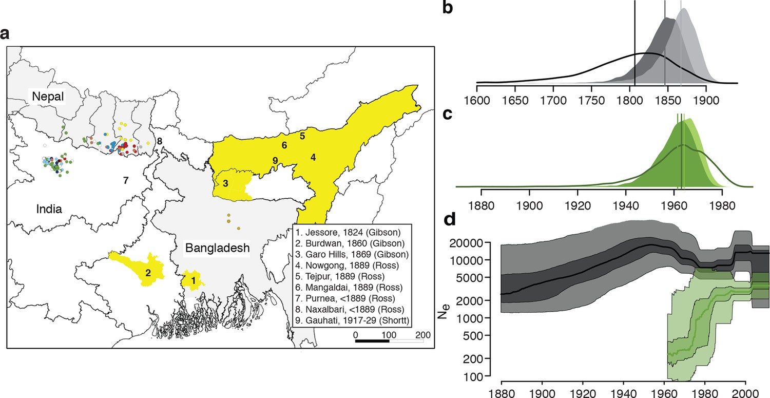
History and geography of Indian subcontinent L. donovani.
(a) Location of the patients from which the 204 L. donovani genomes were isolated, and of historical Kala-Azar outbreaks. Genetic groups of the parasite isolates are indicated by the colour of the dots representing them, matching those in Figure 2a,c. Sampling dates and locations are summarised in Figure 1—figure supplement 1, and detailed information about each strain including GPS coordinates are given in the source data file. Citations are to historical primary literature reviewed and cited in (Gibson, 1983). Posterior probability distributions of estimated ages for the oldest split in (b) the main population in Bihar and Nepal and (c) the ISC5 group associated with Sb resistance. Dark shading shows estimates under a strict molecular clock, light shading from relaxed molecular clock and lines show relaxed clock results with Bangladeshi and putative hybrid isolates included. (d) Estimated effective population size through time for ISC5 population (green) and the rest of the parasite population (black/grey). Lines show median of posterior distributions, dark and light shading cover 50% and 95% of the posterior density respectively. Dates for all splits on this phylogeny and other results of phylogeographic analysis are shown in Figure 1—figure supplement 2.
Figure 1—figure supplement 1
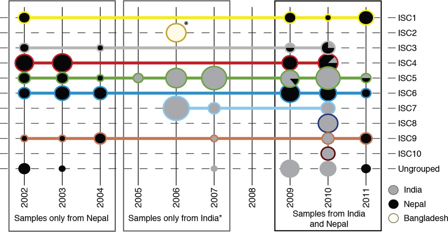
Sampling of genetic groups.
Pie charts indicate the number of samples in each year (columns), for each genetic group (rows) coming from each country (grey shading). Horizontal lines connect and surround isolates of each group, with colours matching the groups shown in panels (b) and (c). *8 samples from Bangladesh were all sampled in 2006, and form a distinct population to Nepalese and Indian isolates (ISC2).
Figure 1—figure supplement 2

Full results of discrete-space, constant population size molecular clock Bayesian phylogeography analysis of core population.
(a) Maximum posterior probability phylogeny, with tips coloured by country of origin for sample (green for India, blue for Nepal), and branches coloured by maximum posterior probability of country reconstructed in discrete phylogeography model. Values on nodes indicate posterior probability of assigned country/colour, with filled circles marking nodes with probability 1. Other panels represent posterior probability distributions for rates of migration (lineage switches per month) from (b) Nepal to India and (c) from India to Nepal. Note the mode (maximum posterior probability estimate) for migration from Nepal is zero, but non-zero migration in the reverse direction is supported.
Figure 2 with 4 supplements

Genealogical history of L. donovani from the ISC.
(a) Maximum-likelihood tree based on SNPs called for 191 strains (see Figure 2—figure supplement 1) from the core population in the Indian subcontinent. Samples are coloured by population assignment, with putative hybrid strains not clustered in the main groups in black. Further analysis confirms the hybrid ancestry of some of these isolates (Figure 2—figure supplement 2). (b) Unrooted phylogenetic network of the L. donovani complex based on split decomposition of maximum-likelihood distances between isolates described here, reference genome isolates and two published Sri Lankan isolates (Zhang et al., 2014). (c) Model-based clustering of 191 isolates from the core population reveals six discrete monophyletic groups, and some groups and other samples of less certain ancestry. Coloured bars show the fraction of ancestry per strain assigned to a given cluster, with colours assigned to the population most closely related to each cluster. More detailed population clustering analysis shows largely congruent results (Figure 2—figure supplements 3 and 4).
Figure 2—figure supplement 1

Flowchart of SNP detection using COCALL.
Overview of the SNP detection method COCALL (COnsensus of SNP CALL). COCALL finds genetic variants that show a concordant signal over five different SNP callers (Cortex, Freebayes, GATK, Samtools Mpileup and Pileup). See supplementary methods for details.
Figure 2—figure supplement 2
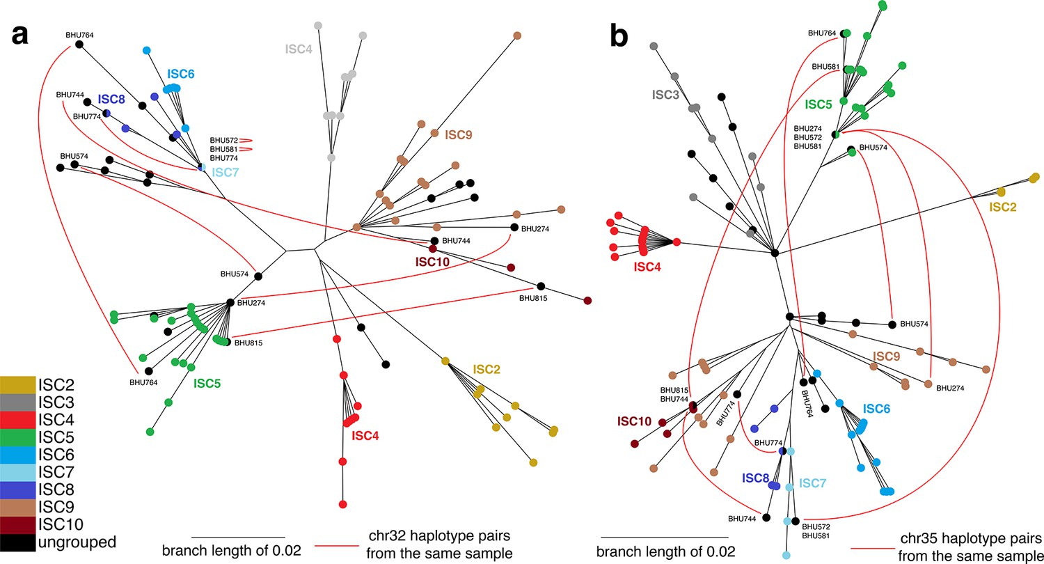
Haplotype networks for core population isolates.
Haplotype networks indicate putative hybrids as isolates with ancestry from multiple distinct populations. Chromosomal haplotype neighbour-joining networks of the phased data for the core population were constructed using the R ape package. Each node represents one haplotype variant for (a) chromosome 32 and (b) chromosome 35, coloured by group. Black lines are network edges and red lines connect haplotype variants from the same isolate for selected isolates where haplotypes appear in different parts of the network (with isolate names shown). Six ungrouped isolates (BHU815/0, BHU764/0cl1, BHU274/0, BHU574cl4, BHU581cl2, BHU572cl3) have mixed ancestry from ISC5 and other groups, and two (BHU744/0 and BHU774/0) have a mix of ISC6/7/8/9/10 haplotypes. No mixing among ISC2/3/4 was evident.
Figure 2—figure supplement 3

Haplotype similarity for core population isolates.
Heatmap showing the mean expected number of haplotypes shared between pairs of core population isolates. Samples listed on the y-axis are haplotype donors to those on the x-axis. 18,747 phased genotypes at 2397 SNPs sites were computed with Chromopainter v0.0.2 using recombination rates from PHASE for 79 haplotype chunks with c=0.00054 effective chunks. This image confirms six discrete populations ISC2-7 and illustrates complex ancestry in certain samples not belonging to these groups.
Figure 2—figure supplement 4
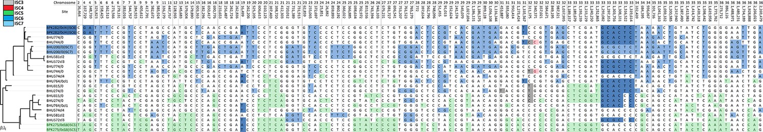
Mosaic ancestry patterns in eight putative hybrid L. donovani isolates.
Representative samples from three potentially parental groups (BPK282/0cl4, ISC6; BHU200/0, ISC7; BPK275/0cl18, ISC5) were compared to eight putative hybrid samples (BHU815/0, BHU764/0cl1, BHU274/0, BHU574cl4, BHU581cl2, BHU572cl3, BHU744/0 and BHU774/0). To the left is a maximum-likelihood tree constructed with RAxML showing the evolutionary history of the aligned haplotypes. The table shows a set of SNPs for which ChromoPainter assigned ancestry probability values >0.4 in any of these eight hybrids. Individual SNPs are coloured if the sample had an ancestry probability >0.4: uncoloured ones represent those observed in multiple ISC populations. All isolates have mixed ancestry from the two groups, but four isolates (BHU574cl4, BHU764/0cl1, BHU815/0 and BHU274/0) have haplotypes that appear to have a more complex origin.
Figure 3 with 3 supplements
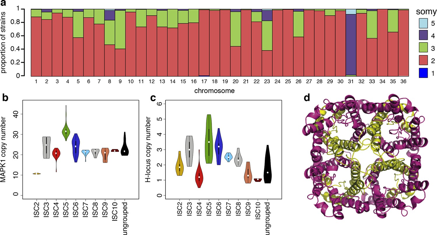
Structural variations in ISC L. donovani.
(a) Stacked barplots per chromosome showing the proportion of ISC strains that are monosomic, disomic, trisomic, tretrasomic or pentasomic for the respective chromosome. A full breakdown of somy per strain is presented in Figure 3—figure supplement 3, and a complete catalogue of other structural variants in Figure 3—figure supplement 1. Violin plots showing the copy number of MAPK1 (b) and H-locus (c) per ISC group, except for ISC1 where these amplicons were absent. These amplicons are intra-chromosomal (Figure 3—figure supplement 2). (d) Tetrameric protein model of the transport protein aquaglyceroporin-1. The C-terminus part that is affected by the 2-nucleotide frameshift found in all ISC5 isolates is shown in magenta. Image was created using PyMOL version 1.50.04 (Schrödinger).
Figure 3—figure supplement 1
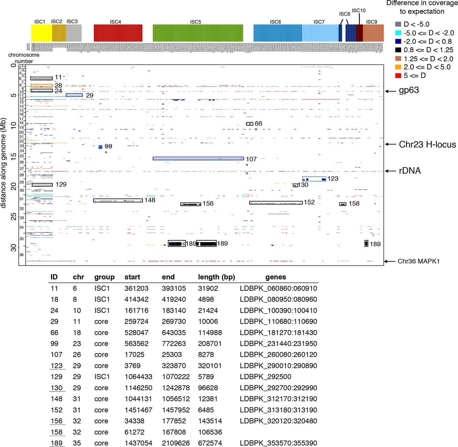
Copy number variants in all 206 genomes.
The position in the genome is shown on the y-axis, while individual isolates are shown on the x-axis. Colours of each copy number variant (CNV) represent the haploid depth variation (D) compared to the median depth for that chromosome (see legend for colour key). When the depth of the majority of the strains is high like the episome in ch23, this appears as a reduced depth in the strains that lack the episome. The length of each CNV is reflected by its length along the y-axis (i.e. thickness of the line). Four major CNVs – gp63, rDNA, an episome in ch23 and the MAPK amplification – are indicated with arrows. Group-specific copy number variants were highlighted with a box and numbered – detailed information about these CNVs are given in the table. The 206 samples included here are 204 ISC samples with L. infantum JPCM5 (MCAN/ES/1998/LLM-877) and L. donovani LV9 (MHOM/ET/1967/HU3) for reference.
Figure 3—figure supplement 2
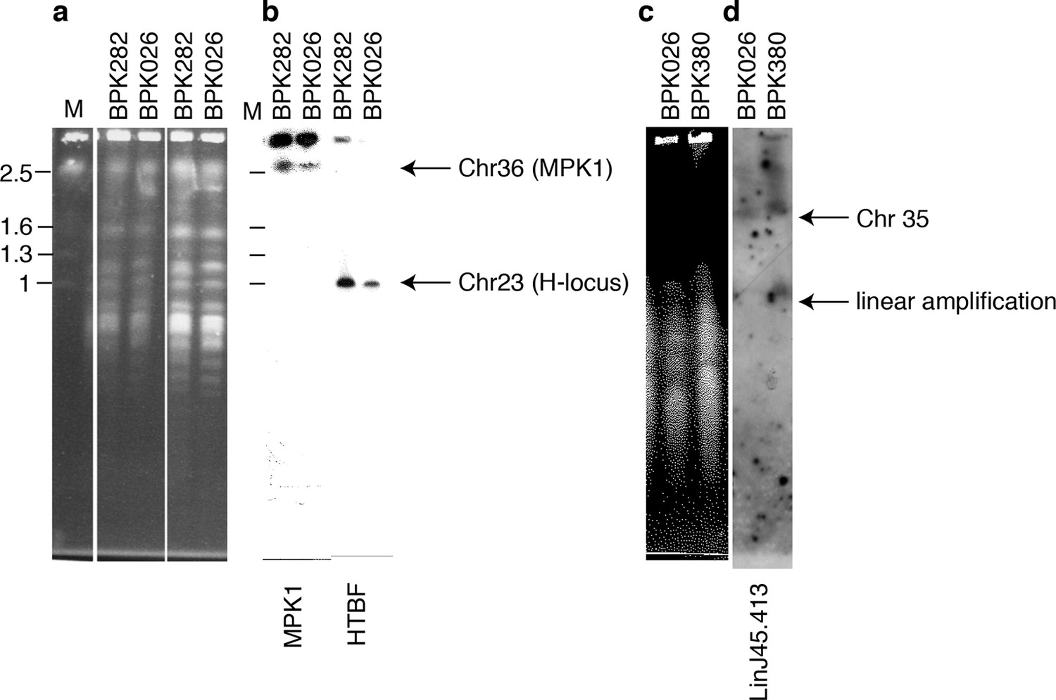
Copy number variation by intrachromosomal tandem duplication or extrachromosomal linear amplification in clinical isolate.
(a, c) Chromosomes from L. donovani BPK282/0cl4 (ISC6), BPK380/0 (ISC9) and BPK026/0cl5 (ISC1) were separated by pulsed-field gel electrophoresis (PFGE). (b) The MAPK1-locus and H-locus were detected by southern blot hybridization with probes specific for MAPK1 or HTBF, respectively. Hybridization was only observed in fragments of lengths equal to those of chr36 (~2.5 Mb) and chr23 (~1 Mb) and no additional smaller fragments were observed, indicating the absence of extra-chromosomal amplifications. (d) In contrast, linear extrachromosomal amplification (as evidenced by a second and smaller band) is shown for chromosome 35 in BPK380/0 by hybridization of a probe specific to the LinJ35.4130 gene.
Figure 3—figure supplement 3
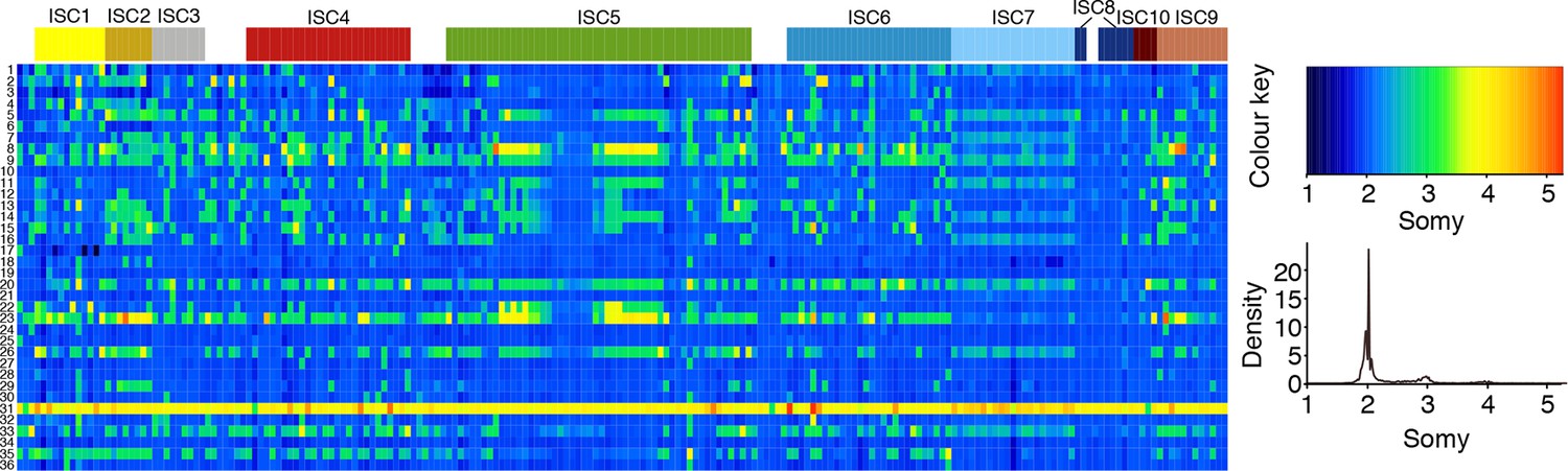
Chromosome number variation in L. donovani in the ISC.
Average number of chromosomes found within each cell culture for each of the 36 chromosomes (y-axis) and each of the 204 L. donovani strains (x-axis). Samples are coloured by population assignment following Figure 1c, with strains not clustered in the main populations shown in white.
Figure 4
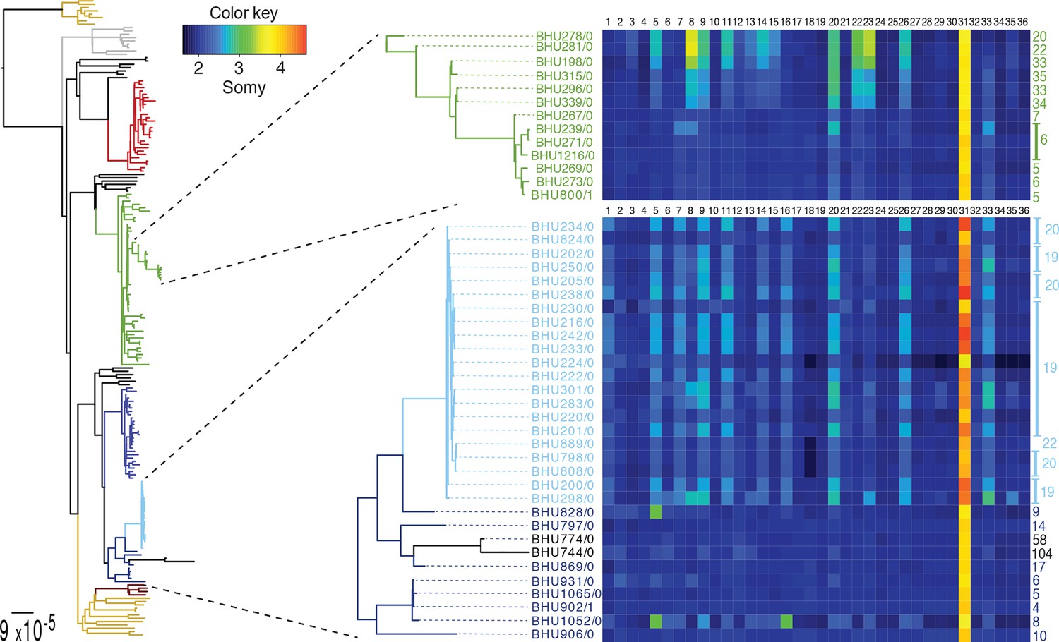
SNP heterozygosity and somy variation in two subclades.
Two subclades show an expansion of polysomic strains from disomic ancestors (below) and an expansion of disomic strains from polysomic ancestors (above). Somy variation per chromosome (1–36; above heatmap) and the total number of heterozygote SNPs (right to heatmap) are shown for each individual strain.
Tables
Table 1
Small indels. The first half of the table summarises the numbers and types of indels detected in each group. The second half of the table shows the proportion of samples within a cluster that share each group-specific coding-region indel.
| 1. Number of indels | ISC002 | ISC003 | ISC004 | ISC005 | ISC006 | ISC007 | ISC008 | ISC009 | ISC010 | ||
| Total number ofindels found within each group | 58 | 60 | 73 | 79 | 65 | 55 | 55 | 84 | 60 | ||
| Number of group-specific Indels shared by part of the strains of that group | 9 | 5 | 11 | 12 | 7 | 0 | 8 | 22 | 7 | ||
| Number of group-specific Indels shared by all the strains of that group | 6 | 1 | 3 | 3 | 0 | 0 | 0 | 0 | 2 | ||
| Number of group-specific Indels within coding regions | 0 | 1 | 2 | 3 | 4 | 0 | 1 | 3 | 1 | ||
| 2. Indels within coding region | |||||||||||
| Gene ID | Gene product | Position | Type | ||||||||
| LdBPK_310030 | Aquaglyceroporin | Ld31_0007774 | 2 | 0.04 | |||||||
| LdBPK_310030 | Aquaglyceroporin | Ld31_0007735 | 2 | 1 | |||||||
| LdBPK_310030 | Aquaglyceroporin | Ld31_0007662 | 1 | 0.04 | |||||||
| LdBPK_310030 | Aquaglyceroporin | Ld31_0008099 | 2 | 0.11 | |||||||
| LdBPK_291860 | Putative historie H2A | Ld29_0816454 | -2 | 0.25 | |||||||
| LdBPK_040410 | Conserved hypothetical protein | Ld04_0155491 | 3 | 0.08 | |||||||
| LdBPK_070540 | Conserved hypothetical protein | Ld07_0230487 | -3 | 0.12 | |||||||
| LdBPK_190080 | Conserved hypothetical protein | Ldl9_0015151 | 1 | 0.04 | |||||||
| LdBPK_261790 | Conserved hypothetical protein | Ld26_0651748 | 4 | 0.11 | |||||||
| LdBPK_301000 | Conserved hypothetical protein | Ld30_0311376 | -1 | 0.02 | |||||||
| LdBPK_310690 | Conserved hypothetical protein | Ld31_0241951 | -3 | 0.11 | |||||||
| LdBPK_332580 | Conserved hypothetical protein | Ld33_0995960 | 1 | 0.04 | |||||||
| LdBPK_366590 | Conserved hypothetical protein | Ld36_2473775 | -3 | 0.25 | |||||||
| LdBPK_110650 | hypothetical, unknown function | Ldll_0245832 | -3 | 0.56 | |||||||
| LdBPK_292330 | hypothetical, unknown function | Ld29_1008496 | -3 | 0.08 | |||||||
Table A1.1
Number of putative SNPs detected by different numbers of SNP calling tools. A threshold mean number of callers ≥3 was used, which was elevated to ≥4 at soft-masked regions.
| #SNP callers | Count | Cumulative count | Freq | Cumulative Freq |
|---|---|---|---|---|
| 1 | 32,072 | 32,072 | 0.822 | 0.822 |
| 1.4 | 154 | 34,475 | 0.004 | 0.884 |
| 1.5 | 498 | 34,973 | 0.013 | 0.896 |
| 2 | 965 | 36,160 | 0.025 | 0.927 |
| 2.5 | 38 | 36,244 | 0.001 | 0.929 |
| 3 | 476 | 36,757 | 0.012 | 0.942 |
| 3.5 | 114 | 36,935 | 0.003 | 0.947 |
| 4 | 1,019 | 38,046 | 0.026 | 0.975 |
| 4.5 | 179 | 38,347 | 0.005 | 0.983 |
| 5 | 438 | 39,015 | 0.011 | 1 |
Table A1.2
The fraction of discordant true and false SNPs between COCALL and GATK population-based variant calling. COCALL had a greater proportion of true SNPs – confirmed by visual inspection of mapping reads – both in terms of the number of variant sites, and across the population of samples.
| SNP caller | Sites | Mutations | ||
|---|---|---|---|---|
| True | False | True | False | |
| COCALL | 106 | 33 | 991 | 118 |
| 76.3% | 23.7% | 89.4% | 10.6% | |
| GATK population caller | 33 | 106 | 118 | 991 |
| 23.7% | 76.3% | 10.6% | 89.4% | |
Table A1.3
The rate of SNP calling for different combinations of read libraries of samples BPK282/0cl4, BPK087/0cl11 and BPK275/0cl18. BPK282/0cl4 was the reference genome strain and so should possess only heterozygous SNPs, and so its variant discovery rate was substantially lower. COCALL identified more rare variant SNPs in mixed libraries.
| Read library combinations | Unique to COCALL | Shared | Unique to GATK population caller | ||
|---|---|---|---|---|---|
| BPK282/0cl4 | BPK275/0cl18 | BPK087/0cl11 | |||
| 89% | 11% | 14 | 140 | 6 | |
| 80% | 20% | 7 | 182 | 7 | |
| 70% | 30% | 6 | 191 | 7 | |
| 60% | 40% | 9 | 193 | 7 | |
| 50% | 50% | 7 | 194 | 7 | |
| 40% | 60% | 5 | 196 | 6 | |
| 30% | 70% | 7 | 191 | 6 | |
| 20% | 80% | 7 | 178 | 8 | |
| 11% | 89% | 9 | 145 | 6 | |
| 89% | 11% | 10 | 50 | 5 | |
| 80% | 20% | 11 | 112 | 5 | |
| 70% | 30% | 5 | 129 | 4 | |
| 60% | 40% | 7 | 131 | 5 | |
| 50% | 50% | 7 | 131 | 6 | |
| 40% | 60% | 6 | 132 | 6 | |
| 30% | 70% | 5 | 133 | 6 | |
| 20% | 80% | 4 | 130 | 6 | |
| 11% | 89% | 4 | 127 | 6 | |
| 89% | 11% | 15 | 64 | 3 | |
| 80% | 20% | 14 | 107 | 4 | |
| 70% | 30% | 4 | 129 | 3 | |
| 60% | 40% | 4 | 132 | 3 | |
| 50% | 50% | 3 | 133 | 4 | |
| 40% | 60% | 3 | 132 | 5 | |
| 30% | 70% | 4 | 131 | 4 | |
| 20% | 80% | 3 | 130 | 5 | |
| 11% | 89% | 3 | 126 | 6 | |
Table A1.4
The probabilities of observing alleles at a specific frequency in the core population and ISC1. We assessed whether or not the SNPs we discovered in our sample of ISC L. donovani were likely to be representative of the variation existing in the wider population of parasites circulating in the ISC. We first assessed the chance of discovering alleles at frequency f as 1-(1-f)^2n in the core population (n=191) and ISC1 (n=12) sample sets (Gutenkunst et al., 2009). As a second approach, we evaluated the chance of sampling at least one derived allele in n sampled chromosomes (as above) assuming these come from a population of size N=1000 following a hypergeometric distribution (Tennessen et al., 2012). Both approaches confirm we have good power (>99% probability) of sampling alleles with population frequencies as low as 1.2% in the core population, but are likely to miss many variants in ISC1.
| Allele Frequency | P(derived allele)=1-(1-f)2n | | ||
|---|---|---|---|---|
| P(derived allele)=1 – | ||||
| Core population | ISC1 | Core population | ISC1 | |
| 0.001 | 0.318 | 0.024 | 0.382 | 0.024 |
| 0.002 | 0.535 | 0.047 | 0.618 | 0.047 |
| 0.003 | 0.683 | 0.07 | 0.91 | 0.07 |
| 0.004 | 0.784 | 0.092 | 0.945 | 0.092 |
| 0.005 | 0.853 | 0.113 | 0.966 | 0.115 |
| 0.006 | 0.9 | 0.134 | 0.979 | 0.136 |
| 0.007 | 0.932 | 0.155 | 0.987 | 0.157 |
| 0.008 | 0.953 | 0.175 | 0.992 | 0.177 |
| 0.009 | 0.968 | 0.195 | 0.997 | 0.197 |
| 0.01 | 0.978 | 0.214 | 0.999 | 0.217 |
| 0.012 | 0.99 | 0.252 | 0.999 | 0.254 |
| 0.015 | 0.997 | 0.304 | 0.999 | 0.307 |
| 0.021 | 0.999 | 0.399 | 0.999 | 0.403 |
| 0.024 | 0.999 | 0.442 | 1 | 0.446 |
| 0.029 | 0.999 | 0.507 | 1 | 0.511 |
| 0.038 | 0.999 | 0.605 | 1 | 0.61 |
| 0.039 | 0.999 | 0.615 | 1 | 0.619 |
| 0.04 | 1 | 0.625 | 1 | 0.629 |
| 0.049 | 1 | 0.701 | 1 | 0.705 |
| 0.065 | 1 | 0.801 | 1 | 0.805 |
| 0.092 | 1 | 0.901 | 1 | 0.904 |
| 0.173 | 1 | 0.99 | 1 | 0.99 |
| 0.272 | 1 | 1 | 1 | 1 |
Table A1.5
The percentage of SNP pairs for all pairs on the same chromosome for which both SNPs occur within a block, for different block sizes (kb) for Cortex, GATK, Samtools Mpileup and Pileup (Supplementary Table 6). Singletons may have clustered for Samtools Pileup, but not for Cortex, GATK or Samtools Mpileup. The mean distance was calculated the average distance between SNPs of the given type on the same chromosome. Non-rare SNPs were those found in three or more samples.
SNP Caller | SNP type | Block size (kb) | ||||||||
|---|---|---|---|---|---|---|---|---|---|---|
0.01 | 0.1 | 0.5 | 1 | 5 | 10 | 50 | 100 | 500 | ||
Cortex | Non-rare | 0.0 | 0.3 | 0.9 | 1.1 | 1.7 | 3.4 | 9.6 | 17.0 | 61.5 |
Doubletons | 1.5 | 1.5 | 1.5 | 1.5 | 3.1 | 3.1 | 10.8 | 13.8 | 64.6 | |
Singletons | 0.0 | 0.0 | 0.0 | 0.0 | 3.8 | 3.8 | 23.1 | 30.8 | 80.8 | |
All | 0.0 | 0.3 | 0.9 | 1.1 | 1.7 | 3.3 | 9.6 | 17.0 | 61.5 | |
GATK | Non-rare | 0.0 | 0.1 | 0.2 | 0.3 | 1.1 | 2.1 | 9.3 | 17.8 | 64.4 |
Doubletons | 1.3 | 1.3 | 1.3 | 1.3 | 1.3 | 1.3 | 5.3 | 13.3 | 61.3 | |
Singletons | 0.0 | 0.0 | 0.0 | 0.0 | 1.1 | 3.2 | 11.8 | 18.3 | 77.4 | |
All | 0.0 | 0.1 | 0.2 | 0.3 | 1.1 | 2.1 | 9.3 | 17.8 | 64.4 | |
Samtools Mpileup | Non-rare | 0.0 | 0.1 | 0.3 | 0.4 | 1.2 | 2.2 | 9.5 | 17.9 | 64.4 |
Doubletons | 0.0 | 0.0 | 0.0 | 0.0 | 6.7 | 6.7 | 6.7 | 20.0 | 60.0 | |
Singletons | 0.0 | 0.0 | 0.0 | 0.0 | 9.1 | 9.1 | 9.1 | 9.1 | 81.8 | |
All | 0.0 | 0.1 | 0.3 | 0.4 | 1.2 | 2.2 | 9.5 | 17.9 | 64.4 | |
Samtools Pileup | Non-rare | 0.0 | 0.1 | 0.2 | 0.3 | 1.1 | 2.1 | 9.3 | 17.8 | 64.4 |
Doubletons | 2.6 | 3.3 | 3.3 | 3.3 | 5.3 | 6.6 | 11.8 | 21.1 | 63.2 | |
Singletons | 0.8 | 4.4 | 5.2 | 5.2 | 5.7 | 6.3 | 13.4 | 24.9 | 71.6 | |
All | 0.0 | 0.1 | 0.2 | 0.3 | 1.1 | 2.1 | 9.3 | 17.8 | 64.5 | |
Table A1.6
The transition (Ti) and transversion (Tv) mutation rates and Ti/Tv ratio across five SNP callers (Cortex, Freebayes, GATK, Samtools Mpileup, Samtools Pileup). SNP sets were selected from the intersection of the SNP calling methods marked X on the corresponding columns (for example, the first row uses the intersection of SNPs called by all five methods). The independent genome assembly and haplotype-based variant calling scheme utilised by Cortex complemented other calling methods based on Smalt assemblies well, based on the increase of the Ti/Tv ratio.
| Cortex | Freebayes | GATK | Samtools mpileup | Samtools pileup | Ti | Tv | Ti/Tv |
|---|---|---|---|---|---|---|---|
| X | X | X | X | X | 9141 | 3336 | 2.74 |
| X | X | X | X | 9229 | 3411 | 2.71 | |
| X | X | X | X | 9150 | 3418 | 2.68 | |
| X | X | X | 9239 | 3499 | 2.64 | ||
| X | X | X | X | 9323 | 3832 | 2.43 | |
| X | X | X | 9418 | 3951 | 2.38 | ||
| X | X | X | 9339 | 3960 | 2.36 | ||
| X | X | 9436 | 4127 | 2.29 | |||
| X | X | X | X | 9194 | 4426 | 2.08 | |
| X | X | X | 9221 | 4591 | 2.01 | ||
| X | X | X | 9289 | 4628 | 2.01 | ||
| X | X | 9342 | 4841 | 1.93 | |||
| X | X | X | 9507 | 6899 | 1.38 | ||
| X | X | 9642 | 7536 | 1.28 | |||
| X | X | 10,399 | 13,101 | 0.79 | |||
| X | 13,351 | 28,388 | 0.47 | ||||
| X | 1,904,004 | 3,340,432 | 0.57 | ||||
| X | 152226 | 553,889 | 0.27 | ||||
| X | 41,107 | 137,315 | 0.30 | ||||
| X | 42,902 | 153,295 | 0.28 |
Table A2.1
Somy status of 36 chromosomes in 206 strains (204 with JPCM5 and LV9). The range of monosomy, disomy, trisomy, tetrasomy and pentasomy was defined to be the haploid normalized chromosome depth dch of dch < 0.65, 0.65 ≤ dch < 1.25, 1.25 ≤ dch < 1.75, 1.75 ≤ dch < 2.25 and 2.25 ≤ dch < 2.75.
| Count | Percentage | |
|---|---|---|
| Monosomy | 2 | 0.03 |
| Disomy | 5851 | 78.90 |
| Trisomy | 1229 | 16.57 |
| Tetrasomy | 310 | 4.18 |
| Pentasomy | 24 | 0.32 |
Table A2.2
Pearson’s correlation (r2) between SNP, CNV, indels and somy diversity. The dependency of the correlation on the normalised pairwise distance is shown: this was determined from the median normalised pairwise distance based on SNP data. The Mantel correlation tests showed values that were consistent with the correlations.
| Type | #samples | Normalised pairwise distance threshold | Correlation (r2) | P value |
|---|---|---|---|---|
| SNP-INDEL | 191 | 0 | 0.433 | 0.00E+00 |
| 57 | 0.15 | 0.301 | 2.91E-254 | |
| 33 | 0.3 | 0.271 | 8.23E-77 | |
| 191 | Mantel test | 0.420 | 0.001 | |
| PLO-SNP | 191 | 0 | 0.073 | 0.00E+00 |
| 57 | 0.15 | 0.152 | 2.69E-118 | |
| 33 | 0.3 | 0.304 | 9.62E-88 | |
| 191 | Mantel test | 0.060 | 0.001 | |
| PLO-INDEL | 191 | 0 | 0.024 | 3.88E-197 |
| 57 | 0.15 | 0.040 | 2.43E-30 | |
| 33 | 0.3 | 0.072 | 1.96E-19 | |
| 191 | Mantel test | 0.016 | 0.001 | |
| CNV-SNP | 191 | 0 | 0.289 | 0.00E+00 |
| 57 | 0.15 | 0.263 | 7.53E-218 | |
| 33 | 0.3 | 0.393 | 4.52E-120 | |
| 191 | Mantel test | 0.272 | 0.001 | |
| CNV-PLO | 191 | 0 | 0.121 | 0.00E+00 |
| 57 | 0.15 | 0.150 | 1.96E-116 | |
| 33 | 0.3 | 0.183 | 1.59E-49 | |
| 191 | Mantel test | 0.103 | 0.001 | |
| CNV-INDEL | 191 | 0 | 0.099 | 0.00E+00 |
| 57 | 0.15 | 0.087 | 2.34E-66 | |
| 33 | 0.3 | 0.108 | 1.04E-28 | |
| 191 | Mantel test | 0.084 | 0.001 |
Table A2.3
Correlation between CNV and ploidy of chromosomes in 206 strains: the duplication threshold was 0.5. p values <0.02 were observed for chromosomes 1, 2, 3, 17, 19, 20, 21 and the whole genome.
| Correlation (r2) | P value | |
|---|---|---|
| chromosome | 0.027 | 7.03E-46 |
| 1 | 0.039 | 4.23E-03 |
| 2 | 0.202 | 1.21E-11 |
| 3 | 0.074 | 7.81E-05 |
| 4 | 0.003 | 4.31E-01 |
| 5 | 0 | 9.30E-01 |
| 6 | 0.004 | 3.86E-01 |
| 7 | 0.003 | 4.68E-01 |
| 8 | 0.001 | 6.05E-01 |
| 9 | 0.001 | 7.32E-01 |
| 10 | 0.015 | 7.77E-02 |
| 11 | 0.002 | 4.88E-01 |
| 12 | 0.005 | 3.16E-01 |
| 13 | 0.001 | 6.57E-01 |
| 14 | 0.001 | 7.31E-01 |
| 15 | 0.001 | 7.42E-01 |
| 16 | 0.009 | 1.81E-01 |
| 17 | 0.036 | 6.06E-03 |
| 18 | 0.005 | 3.23E-01 |
| 19 | 0.077 | 5.41E-05 |
| 20 | 0.064 | 2.51E-04 |
| 21 | 0.027 | 1.87E-02 |
| 22 | 0.009 | 1.87E-01 |
| 23 | 0.007 | 2.42E-01 |
| 24 | 0 | 9.68E-01 |
| 25 | 0.009 | 1.87E-01 |
| 26 | 0.017 | 5.97E-02 |
| 27 | 0.009 | 1.85E-01 |
| 28 | 0.001 | 6.80E-01 |
| 29 | 0.009 | 1.67E-01 |
| 30 | 0.003 | 4.28E-01 |
| 31 | 0.004 | 3.77E-01 |
| 32 | 0.005 | 3.28E-01 |
| 33 | 0.011 | 1.41E-01 |
| 34 | 0.001 | 7.61E-01 |
| 35 | 0.011 | 1.35E-01 |
| 36 | 0.016 | 7.38E-02 |
Additional files
-
Supplementary file 1
DNA samples and their origin.
DNA samples are ordered according to their classification into genetic populations as described in the materials and methods section. The number after the last forward slash in the isolate name indicates when the sample was isolated from the patient in terms of months after onset of a one-month treatment. Patients were followed up for 12 months to assess treatment outcome, with a few exceptions that were lost to follow up and for which the last known outcome is shown mentioning the last recorded time point. The SSG activity index is calculated by dividing the IC50 of a specific strain by the IC50 of BPK206/0cl10 (a sensitive control included in all SSG-susceptibility tests). Activity indexes above 3 are considered to indicate SSG-resistance. MIL: Miltefosine, SSG: sodium stibogluconate, P: passage number, x: unknown number of passages between isolation and shipment to research institute for DNA preparation.
- https://doi.org/10.7554/eLife.12613.017
-
Supplementary file 2
(a) Numbers and types of mutations in the core population compared to genetically distinct strains LV9 (MHOM/ET/1967/HU3) and JPCM5 (MCAN/ES/1998/LLM-877), as well as the ISC1/2. N/S ratio denotes the number of nonsynonymous SNPs divided by the synonymous ones.
The 'LV9+JPCM5-191 lineage' refers to homozygous SNPs occurring in the core population ancestral branch only since its divergence with LV9 and JPCM5. The 'ISC1-191 lineage' refers to fixed homozygous SNPs between all of the core population and all of ISC1. The 'ISC2-183 lineage' refers to fixed homozygous SNPs between ISC2 (Bangladesh) and ISC3/4/5/6/7/8/9/10 and ungrouped isolates (India or Nepal). (b) Number of SNPs unique to each population or lineage. SNPs were determined as unique where their intraspecific frequency was >0.95 and <0.05 in all other samples (excluding ungrouped samples). The number of samples did not reflect the number of SNPs or haplotypes: haplotype diversity was >0.99 for all groups except ISC7 (0.34). (c) Genes ordered by ID with two or more SNPs and π/kb>1. The non-synonymous variant V185M in a NADH-flavin oxidoreductase/NADH oxidase gene (LdBPK_120730) was present here in the ISC1/2/3 as well as previously being observed in Kenyan L. donovani (Downing et al., 2012). 956 genes had at least one SNP, of which 566 had SNPs that were not singletons. Only 63 genes contain ≥2 SNPs and 12 genes contain ≥3 SNPs. (d) Mean numbers of SNP differences within and between groups. Rows and columns denote comparisons: within populations, the mean number of SNPs between strain pairs (π) is shown; and between populations, the mean number of SNPs between samples from each population is given. Within the core population, there was an excess of singletons (Tajima’s D=-2.2, p<0.01, Fu and Li's D=-0.78, Fu and Li’s F=-1.87: the values were the same with either JPCM5 or LV9 as the outgroup). 62.6% of SNPs occurred in one sample only and the correlation of the number of homozygous and heterozygous SNPs per sample was small (r2=0.005). 291 distinct haplotypes out of a maximum possible of 382 were resolved in the phased SNPs, with a resulting haplotype diversity (Hd) of 0.994. Nepalese samples were on average more diverse compared to the Indian ones (π=84.3 per Mb vs 66.5, Hd=0.996 vs 0.982). ISC6 was restricted to Nepal (π=12.2 per Mb). (e) Branch distances between groups using the 2 population (f2) statistic. The scaled correlation in allele frequencies were computed for each reference group (top row) and groups (first column). ISC9 and ISC10 were examined together as one group. The distribution of allele sharing across ISC3/4/5/6 in subsets of trios was compared to that for ISC2 using F-statistics. The relative pairwise correlation in allele frequencies between populations using the f2 test indicated ISC2 as the most consistently divergent population and also highlighted distinctive allele frequencies in the recently emerged Indian ISC7 group. In contrast, groups with possible admixture (ISC9 and ISC10) had much shorter branch lengths. (f) f4 ratios for candidate admixed populations for mixture from ISC5, ISC6 and ISC7.Each ratio was computed as with A and B as either ISC6 or ISC7. Populations X were the 6 samples identified as possible mixtures of the ancestors of ISC5 and ISC6/7: BHU815/0, BHU764A1, BHU274/0, BHU574cl4, BHU581cl2, and BHU572cl3. The gene flow from ISC5 was the f4 ratio and that from B (ISC6 or ISC7) was 1-f4. As expected, if ISC6 and 7 grouped together relative to other groups (f4>0). f4 statistics were considered to support a particular relationship between four individual isolates if 0.05<f4<0.05. ISC2 clustered with ISC3 much more frequently (66.7%) than any other (ISC4, ISC5, ISC6 all 22.2% each). ISC3 had drift patterns more similar to ISC4 (44.4%) than ISC6 (22.2%) or ISC5 (0%). ISC4 had greater correlation with ISC5 (44.4%) than ISC6 (22.2%). ISC5 and ISC6 had more similar drift in 66.7% of tests. These values are consistent with the relationship (ISC2,(ISC3,(ISC4,(ISC5,ISC6))))) shown by the phylogenetic analysis. Admixture levels were measured for the six ISC5-ISC6/7 hybrids as a single population using f4 ratios with ISC2, ISC3 and ISC4 as outgroups. The six hybrids were BHU815/0, BHU764A1, BHU274/0, BHU574cl4, BHU581cl2 and BHU572cl3. The fraction of ancestry attributed to ISC5 was 54–56% and to ISC6 was 44–46% for ISC5-ISC6 mixing, and the alternative ISC5-ISC7 mixture had ISC5 at 59–61% and ISC7 at 39–41%. (g) Diagnostic SNPs for ISC7. 20 mutations were unique to ISC7 compared to the other genetically homogeneous populations (ISC2/3/4/6/7/8/9/10) with a ISC7 frequency >0.98 and a non-ISC7 frequency <0.02. Six were nonsynonymous. These SNPs coincided with a distinct chromosome copy number pattern in ISC7. SNPs were assigned to the 5’ and 3’ UTR if they are within 1 Kb of the start or end of the gene (respectively). ISC7 was a recent radiation restricted to India (π=1.8 per Mb). (h) Diagnostic SNPs for ISC5. 32 mutations were unique to ISC5 compared to the other genetically homogeneous populations (ISC2/3/4/6/7/8/9/10), with ISC5 frequency >0.95 and a non-ISC5 frequency <0.05. Eight changes were nonsynonymous. *Nine were previously associated with antimonial resistance, including four samples from this ISC5 dataset (Downing et al., 2011): six of these would change the amino acid sequence. SNPs were assigned to the 5’ and 3’ UTR if they are within 1 Kb of the start or end of the gene (respectively). (i) Diagnostic SNPs for disomic clade within ISC5. 16 diagnostic SNPs unique to a subset of the ISC5 associated with an expansion of disomic strains from polysomic ancestors (BHU1216/0, BHU239/0, BHU271/0, BHU267/0, BHU800/1, BBU269/0, and BHU273/0). Each SNP had a read-depth allele frequency >0.978 within this group and a frequency <0.04 in the other strains not in this group. These SNPs coincided with a distinct chromosome copy number pattern in this group. Ref is the reference genome BPK282/0cl4 allele and Var is the observed derived one. (j) Linkage disequilibrium (LD) and SNP density across chromosomes in the core population. LD was computed as the r2 values between SNP pairs. SD is the standard deviation. The number of homozygous (hom) and heterozygous (het) mutations per chromosome across all 191 samples is shown. LD was markedly higher for chromosome 31, and lower for 1, 6, 7, 8 and 10. The number of recombinant pairs was largest on chr31 (469), which had the highest somy level and was the most SNP-dense chromosome. (k) A genomic map of SNPs in the core population whose ancestry could be assigned to a population. Using the 191x6 ChromoPainter model, the 610 ancestry-informative SNPs were examined to highlight those with probabilities of being donated given ISC group was >0.4: ISC2 (gold), ISC3 (grey), ISC4 (red), ISC5 (green), ISC6 (blue) and ISC7 (light blue). The representative samples used for the 191x6 ChromoPainter model were BD09 (ISC2), NEP123/6 (ISC3), BPK087/0cl1 (ISC4), BPK275/0cl18 (ISC5), BPK282/0cl4 (ISC6) and BHU200/0 (ISC7). SNPs with probabilities <0.4 are uncoloured. For chr32 and chr35, most recombinant pairs could be attributed to the eight ungrouped hybrid isolates. (l) Number and heterozygosity of ancestry-informative SNPs per isolate. The number of homozygous (hom) and heterozygous (het) SNPs distinguishing each core sample (191 total) from six representative samples from each genetically distinct ISC population: ISC2 (BD09), ISC3 (NEP123/6), ISC4 (BPK087/0cl1), ISC5 (BPK275/0cl18), ISC6 (BPK282/0cl4) and ISC7 (BHU200/0). There were 610 informative SNPs with an ancestry probability threshold >0.4. The relative ratio of homozygous and heterozygous SNPs denoted the genetic relatedness of the strains. Samples possessing recent common ancestry with the representative strains had few homozygous SNPs but the same rate of heterozygous SNPs compared to other representative samples. Similarly, samples possessing recent common ancestry with multiple representative samples had fewer homozygous SNPs and no change in the heterozygous SNPs. This was apparent for highlighted ungrouped samples BHU815/0, BHU764A1, BHU274/0, BHU574cl4, BHU581cl2, BHU572cl3 (all ISC5/6/7: green and blue); and BHU744/0, BHU774/0 (ISC6/7: blue). In many groups haplotype segments were shared across isolates widely separated in sampling date. For example, in ISC3, 35 haplotype segments were shared between NEP123/6 (2004), BPK507/0 (December 2009), BPK515/0, BPK518/0 and BPK519/0 (all February 2010); 53 haplotype segments were shared between BPK157/0cl5 (October 2002) and BPK602/0 (February 2011) (both ISC9); 44 between BPK280/0 (August 2003) and BPK615/0 (March 2011; both ungrouped); 31 between BHU274/0 (ungrouped, August 2007) with BHU1199/0 (ISC9, November 2010). (m) Distribution of copying probabilities of SNPs in two representative isolates. Expected copying probabilities from Chromopainter assigning ancestry to SNPs from BHU581/0 (Ungrouped, left) and BPK275/0cl18 (ISC5, right) using probabilities derived from a model assigning SNP ancestry to representative samples from ISC2/3/4/5/6/7. Each column shows the percentage of SNPs assigned to each percentage probability of being donated from each population (eg ISC2) for a particular sample (eg BHU581/0). If many SNPs had high probabilities of being donated from a particular population, this implied that sample shared a recent ancestor with that population. BHU581/0 was a putative ISC5/6/7 hybrid, and had 9.4% of its SNPs with ancestry from ISC6 or ISC7, 7.2% from ISC7, and 10.9% from ISC5. In contrast, BPK275/0cl18 was the representative sample for ISC5, and 44.3% of its SNPs had confident ancestry from ISC5. No SNPs from any comparison were assigned probabilities between 50–95%, hence these rows are omitted from the table. These ancestry patterns indicated that BPK035/0cl1-BPK043/0cl2, BHU1011/0-BHU770/0cl1, BPK280/0-BPK615/0 and BPK158/0cl9 represented ISC4-related isolates but not mixtures. BHU774/0 and BHU744/0, showed evidence of both ISC6- and ISC7-derived segments. The six ungrouped samples (BHU274/0, BHU815/0, BHU764/0cl1, BHU574cl4, BHU572cl3 and BHU581cl2) were sampled between February 2007 and February 2010 and had high numbers of heterozygous SNPs. High heterozygosity could be symptomatic of genetically distinct parents in a hybrid. For example, if BHU572cl3 and BHU581cl2 (both May 2009) were mixes of ISC5 (BHU573/0, May 2009) and ISC7 (BHU200/0, July 2006) then only 16 out of 280 genotypes (BHU572cl3) and 15 out of 278 genotypes (BHU581cl2) would be unexplained. This was evaluated for different haplotype sharing options and matched the timing of samples (BHU572cl3, BHU574cl4 and BHU581cl2 in relation to BHU573/0; BHU815/0 in relation to BHU816/0). SNPs assigned to populations with a high probability in the 191x6 model provided a framework for predicting strain membership as well as admixture. Comparing the relative difference in distributions of homozygous and heterozygous SNPs between candidate parents within the sample set was sufficient to identify shared ancestry where related lineages were sampled, and visible in the aligned genotypes of the six strains with segments of both ISC5 and ISC6 ancestry. (n) Percentage of haplotype segment copies shared within and between groups. Recipients are shown as columns and donors as rows. Groups with complex ancestries received more segments than they donated: ISC8 from ISC5, ISC6 and ISC7; ISC3, ISC9 and ISC10 from ISC5. These 'recipient' groups were also associated with long external branch lengths in phylogenies. The expected probability per SNP in each population for the 191x191 co-ancestry analysis indicated that strains assigned to populations by Structure were assigned the same one with FineStructure (ISC2/3/4/5/6/7): ISC2 (copying probability >99%), ISC3 (>97%), ISC4 (>98%), ISC5 (>99%), ISC6 (>90%) and ISC7 (>97%). Genetically heterogeneous groups showed a higher rate of segments were received than donated from specific populations: ISC8 from ISC5 (11.3% vs 1.7%), ISC6 (16.6% vs 4.7%) and ISC7 (16.5% vs 6.2%). ISC9 (10.0% vs 0.8%) and ISC10 also received more from ISC5 (11.1% vs 2.5%). ISC5 also donated more to ISC3 (11.0% v 1.9%) suggesting possible ancestral genetic exchange, which may be associated with the long branch lengths leading to ISC3. (o) Four-gamete test for recombination. Four gamete tests showed evidence of recombination in the core population and ISC1. 2043 from 117,055 (1.75%) SNP pairs had a recombination signature in the core population. For the subset of 2,015 SNPs with no missing data R=0.7/Mb. The 8 hybrids were BHU815/0, BHU764A1, BHU274/0, BHU574cl4, BHU581cl2, BHU572cl3 (all ISC5+ISC6/7), BHU744/0 and BHU774/0 (both ISC6/7 only). Recombination was evident at 25% of SNPs in ISC1 (184,827 out of 739,581 SNP pairs) based on the four gamete test. This signature varied over 13-fold from chr31 (54.2% of pairs) to chr23 (4%). (p) SNP and indel association with SbV resistance. Fisher exact tests evaluated the association of SbV-resistance with SNPs (coded as the number of derived mutations: 0, 1 or 2) and indels (coded as the diploid number of inserted or deleted (-) basepairs). (q) SNP association with in-vitro SSG phenotype. SNPs with derived alleles in multiple ISC groups with 6+ non-reference genotypes for which the absolute difference in SSG-R and SSG-S allele frequency was >0.1 with the OR (odds ratio) >4 and Benjamini-Hochberg-Yekutieli corrected t-test p value <0.005. SNPs are ordered by chromosome and position. The SSG phenotypes were assessed as ln(EC50) values for the derived (D) and reference (R) alleles. To avoid arbitrarily categorising the sample in vitro SbV phenotypes as R and S using a given threshold EC50 value, we compared the log-scaled EC50 values of each allele pair at the 57 SNPs identified using t-tests (p<0.005): the SbV-R alleles had log-scaled EC50 values of 1.13–1.84 compared to S ones of 0.01–0.50 (Supplementary file 1). Consequently, the 57 SNPs together have power to differentiate SbV-R and SbV-S phenotypes. (r) SNP association with clinical outcome from SSG treatment. SNPs with derived alleles in multiple ISC groups with 6+ non-reference genotypes for which the absolute difference in SSG-cure and SSG-failure allele frequency was >0.1 with the OR (odds ratio) >4. The SNPs are ordered by chromosome and position. The SSG phenotypes were assessed for the derived (D) and reference (R) alleles. We examined lines for which the patient was treated with SSG and was either cured (n=21) or treatment failed (n=14: death, relapse, no response to treatment) to test a null hypothesis that SSG outcome and SNPs were unlinked. An alternative hypothesis was that SSG-cure patients could be infected with SbV-S parasites, and SSG-fail with SbV-R (Supplementary file 2). 32 SNPs were associated with SSG cure (OR>4), including 11 nonsynonymous SNPs, but none at a significant level due to the small sample size. (s) Relative strength of purifying selection between ISC populations. Relative strength of purifying selection between ISC populations (columns 1 and 2) as ascertained as the relative rate of accumulation of derived alleles computed as R for all (top), nonsynonymous (middle) and synonymous (bottom) sites. We tested for differential selective pressures among the ISC groups where observed values of R statistics deviated by at least four standard errors (SE) from the expected value of 1 (Do et al 2015). The genome-wide values are shown along with the weighted block jackknife confidence intervals (lower, median, upper). Derived alleles were more frequent in ISC4 than ISC5, suggesting stronger purifying selection in ISC5. Comparing ISC2 (Bangladesh) to ISC3-7 (Nepal/India), we found a genome-wide (RG) excess of derived alleles had accumulated in the latter (RG=0.74, 6.15*SE). This was not directly attributable to selection because the difference was present in both nonsynonymous (RN=0.59, 4.42*SE) or synonymous sites (RS=0.66, 10.82*SE). ISC3/4/5/6 shared genetic ancestors dating to approximately the same origin, so a comparison of their rates should indicate variation in the relative accrual of derived alleles. Despite possessing the largest sample size (n=52) of all ISC populations, ISC5 gained significantly fewer derived alleles genome-wide compared to ISC3 (RG=0.75, 11.39*SE), ISC4 (RG=0.65, 7.37*SE) and to a lesser extent, ISC6 (RG=0.82, 3.38*SE). This trend was present in both nonsynonymous and synonymous SNPs but not significant for most comparisons (an exception was comparing synonymous changes in ISC5 vs ISC4 (RS=0.37, 7.80*SE). Similarly, the rate of accumulation of homozygous derived SNPs (R2 values) was higher in ISC4 relative to ISC5 (R2G=0.90, 3.87*SE). Antimonial in vitro resistance was highest in ISC5 (ln[EC50]=1.38 ± 1.45) and lowest in ISC4 (0.13 ± 1.12). Consequently, the relative difference in the rate of accumulation of derived alleles in ISC5 that was predominantly isolated in India may reflect different exposure to drug selection compared to ISC4 (mainly from Nepal). Further work is required to quantify this in relation to variable antimonial resistance levels among samples in each population. ISC7 was a genetic subgroup of ISC6 that may be a recent radiation or have undergone a substantial population bottleneck. No genome-wide difference was evident in terms of selction, but fewer derived synonymous SNPs were found in ISC6 (RS=2.18, 4.44*SE), suggestive stronger hitchhiking of alleles in ISC7. (t) Multi-allelic sites. Sites with multiple derived alleles compared to reference genome sample BPK282/0cl4 in the core population (7, top) and ISC1 (10, bottom).
- https://doi.org/10.7554/eLife.12613.018
Download links
A two-part list of links to download the article, or parts of the article, in various formats.
Downloads (link to download the article as PDF)
Open citations (links to open the citations from this article in various online reference manager services)
Cite this article (links to download the citations from this article in formats compatible with various reference manager tools)
Evolutionary genomics of epidemic visceral leishmaniasis in the Indian subcontinent
eLife 5:e12613.
https://doi.org/10.7554/eLife.12613


