Dynamics of genomic innovation in the unicellular ancestry of animals
- Institut de Biologia Evolutiva (CSIC-Universitat Pompeu Fabra), Catalonia, Spain
- Universitat de Barelona, Catalonia, Spain
- Université Paris-Sud/Paris-Saclay, AgroParisTech, France
- University of Hawai'i at Mānoa, United States
- Prefectural University of Hiroshima, Japan
- University of Exeter, United Kingdom
- ICREA, Passeig Lluís Companys, Catalonia, Spain
Figures
Figure 1 with 1 supplement
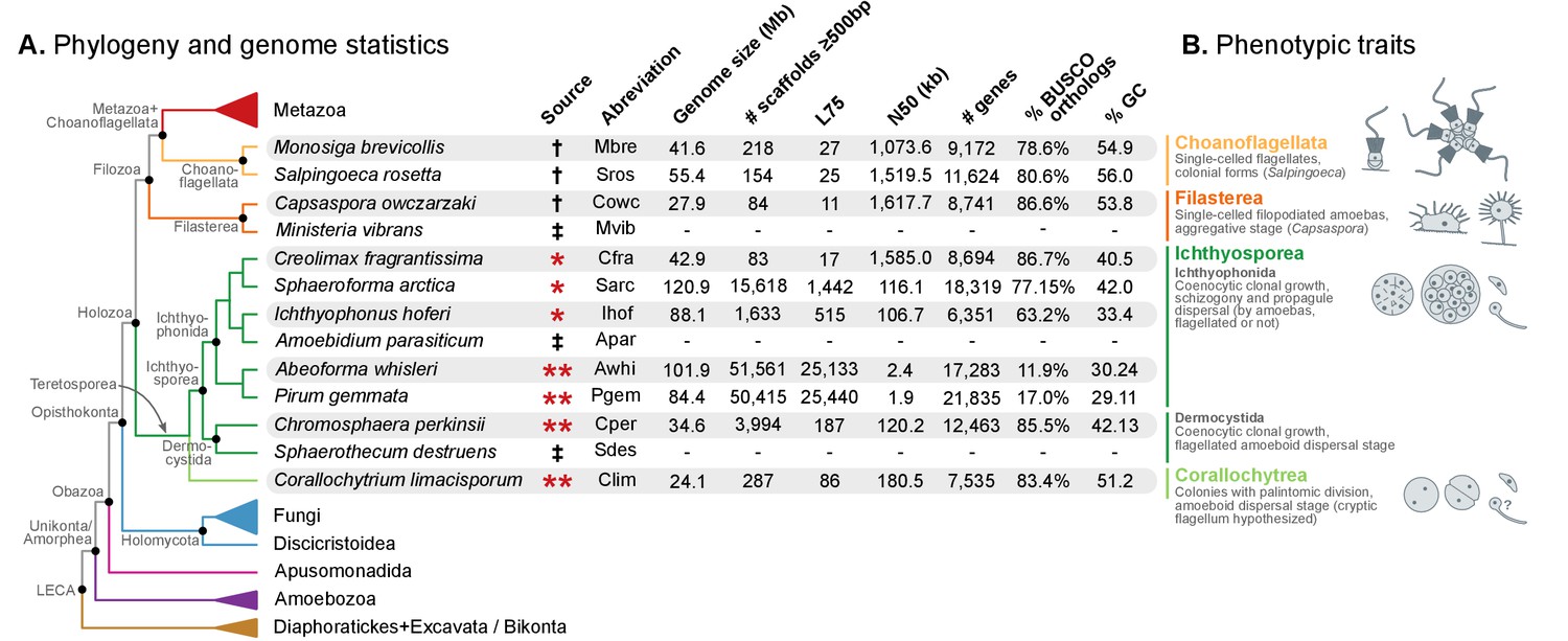
Evolutionary framework and genome statistics of the study.
(A) Schematic phylogenetic tree of eukaryotes, with a focus on the Holozoa. The adjacent table summarizes genome assembly/annotation statistics. Data sources: red asterisks denote Teretosporea genomes reported here; double asterisks denote organisms sequenced for this study; † previously sequenced genomes (King et al., 2008; Fairclough et al., 2013; Suga et al., 2013); ‡ organisms for which transcriptomic data exists but no genome is available (Torruella et al., 2015). (B) Overview of the phenotypic traits of each group of unicellular Holozoa, focusing on their multicellular-like characteristics. For further details, see (Torruella et al., 2015; Mendoza et al., 2002; Marshall et al., 2008; Glockling et al., 2013). Figure 1—source data 1 and 2.
-
Figure 1—source data 1
Table of genome structure statistics, from the data-set of eukaryotic genomes used in the study.
- https://doi.org/10.7554/eLife.26036.004
-
Figure 1—source data 2
List of genome and transcriptome assemblies and annotations, including abbreviations, taxonomic classification and data sources.
Used in Figure 1.
- https://doi.org/10.7554/eLife.26036.005
Figure 1—figure supplement 1
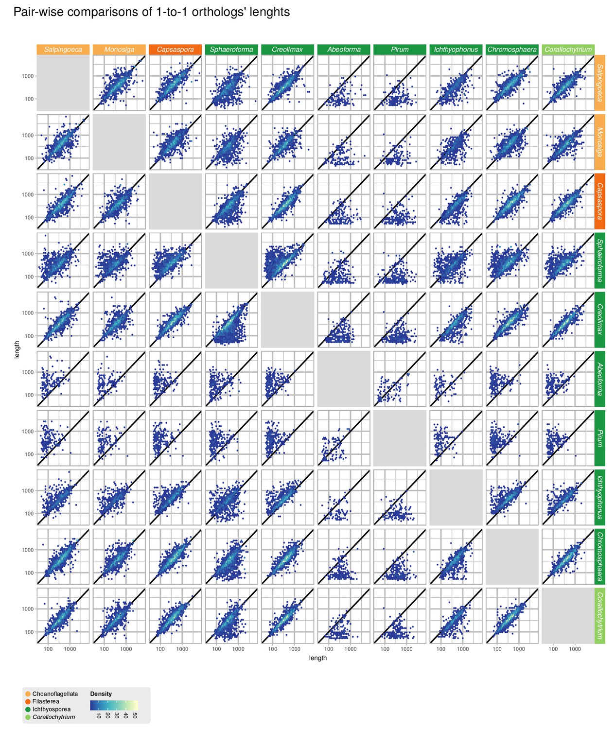
Comparisons of gene length of one-to-one orthologs from pair-wise comparisons of all 10 unicellular Holozoa.
Dots around the diagonal lines indicate that orthologs from both organisms have identical lengths. Note that Abeoforma and Pirum have abundant incomplete orthologous sequences.
Figure 2 with 1 supplement
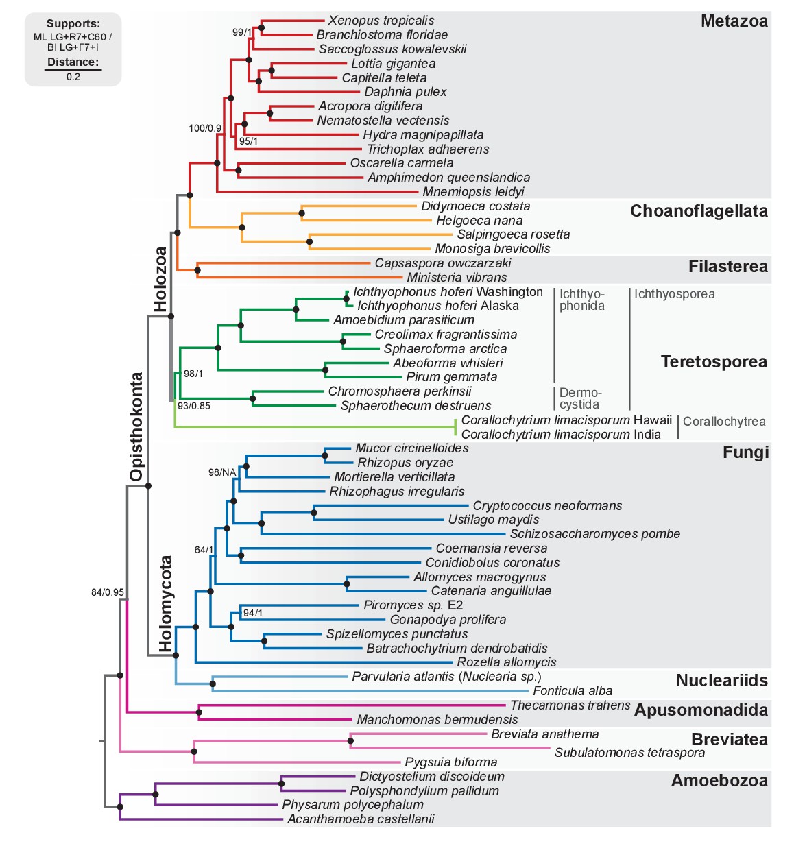
Phylogenomic tree of Unikonta/Amorphea.
Phylogenomic analysis of the BVD57 taxa matrix. Tree topology is the consensus of two Markov chain Monte Carlo chains run for 1231 generations, saving every 20 trees and after a burn-in of 32%. Statistical supports are indicated at each node: (i) non-parametric maximum likelihood ultrafast-bootstrap (UFBS) values obtained from 1000 replicates using IQ-TREE and the LG + R7+C60 model; (ii) Bayesian posterior probabilities (BPP) under the LG+Γ7 + CAT model as implemented in Phylobayes. Nodes with maximum support values (BPP = 1 and UFBS = 100) are indicated by a black bullet. See Figure 2—figure supplement 1 for raw trees with complete statistical supports. Figure 2—source data 1.
-
Figure 2—source data 1
BVD57 phylogenomic dataset (Torruella et al., 2015) including 87 unaligned protein domains (with PFAM accession number) per species.
Used in Fig. 2.
- https://doi.org/10.7554/eLife.26036.008
Figure 2—figure supplement 1
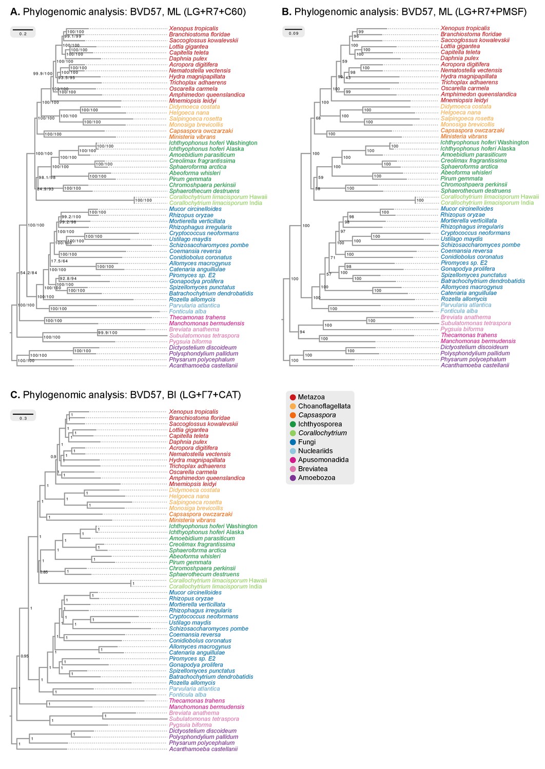
Phylogenomic analysis of the BVD57 matrix using (A) IQ-TREE maximum likelihood and the LG + R7+C60 model (supports are SH-like approximate likelihood ratio test/UFBS, respectively); (B) IQ-TREE maximum likelihood and the LG + R7+PMSF model (fast CAT approximation; non-parametric bootstrap supports); and (C) Phylobayes Bayesian inference under the LG+Γ7 + CAT model (BPP supports).
https://doi.org/10.7554/eLife.26036.009
Figure 3 with 3 supplements
Patterns of genome evolution across unicellular Holozoa.
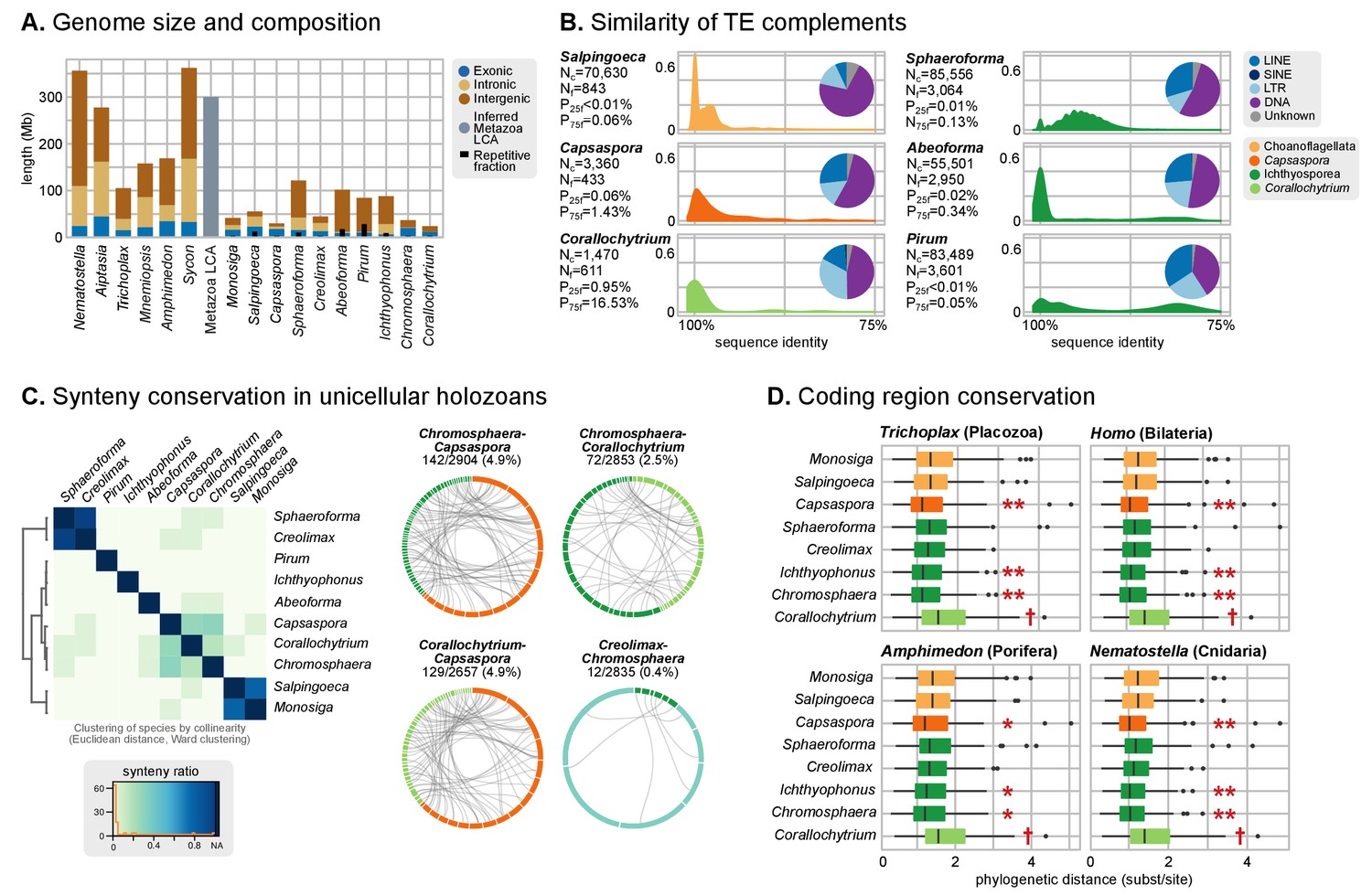
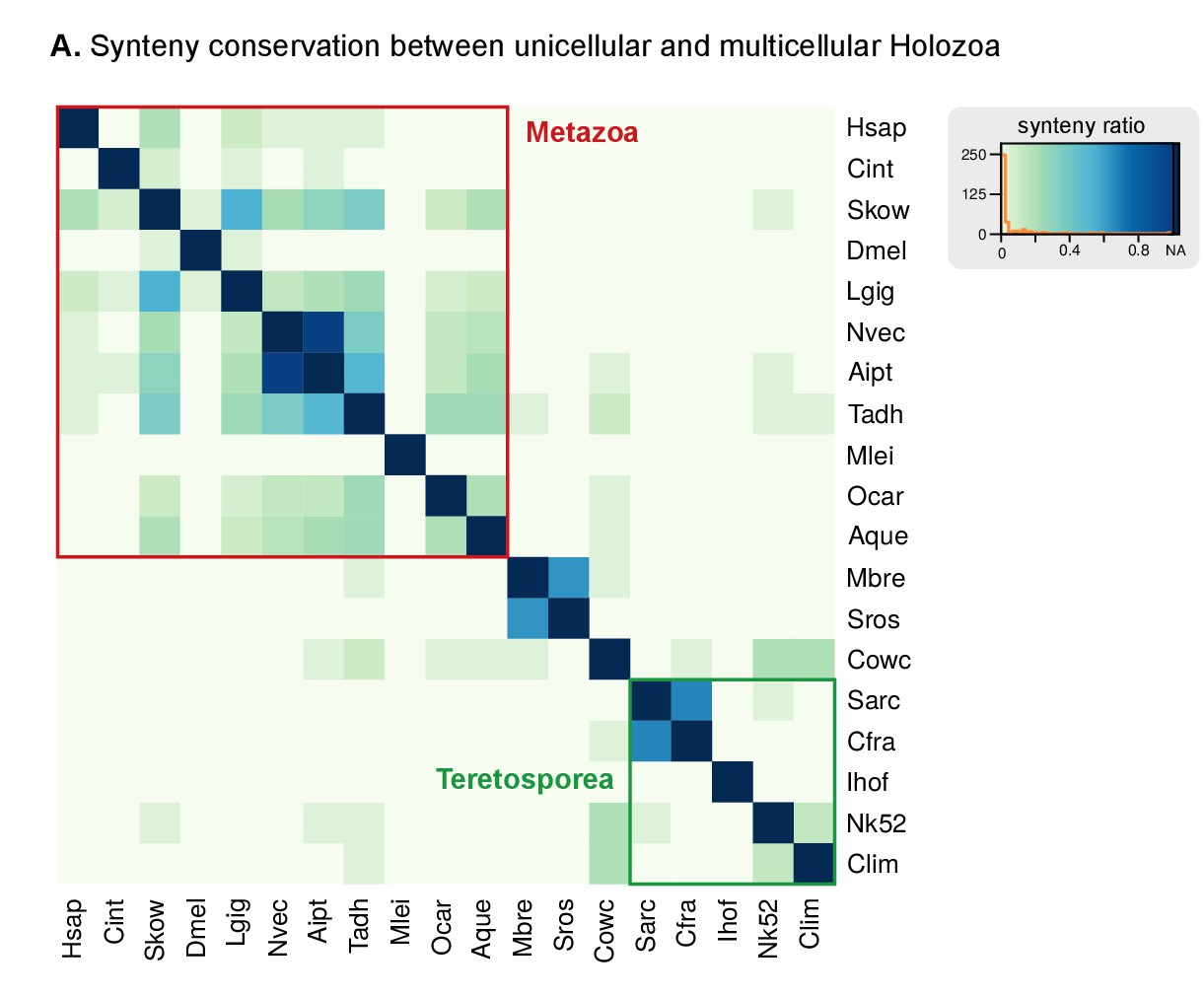
(A) Genome size and composition in terms of coding exonic, intronic and intergenic sequences of unicellular holozoan and selected metazoans. Percentage of repetitive sequences shown as black bars. Genome size of the Metazoa LCA (gray bar) from (Simakov and Kawashima, 2017) (exonic, intronic and intergenic composition not known). (B) Profile of TE composition for selected organisms. Density plots indicate the sequence similarity profile of the TE complement in each organism. Embedded pie-charts denote the relative abundance, in nucleotides, of the main TE superclasses in each genome: retrotransposons (SINE, LINE and LTR), DNA transposons (DNA) and unknown. Nc: total number TE copies in the genome; Nf: number of families to which these belong; P25f and P75f: percentage of most-frequent TE families that account for 25% and 75% of the total number of TE copies, respectively. (C) Heatmap of pairwise microsynteny conservation between 10 unicellular holozoan genomes. Species ordered according the number of shared syntenic genes (Euclidean distances, Ward clustering). At the right: selected pairwise comparisons of syntenic single-copy orthologs between unicellular holozoan genomes. Numbers denote number of syntenic genes, total number of single-copy orthologs, and proportions (%) of syntenic genes per the compared orthologs. Circle segments are scaffolds sharing ortholog pairs, connected by gray lines. (D) Phylogenetic distances between unicellular holozoans and four selected animals: Homo sapiens, Nematostella vectensis, Trichoplax adhaerens and Amphimedon queenslandica. Red asterisks denote organisms that have lower phylogenetic distances to metazoans than one (single asterisk) or both choanoflagellates (double asterisks) (p value < 0.05 in Wilcoxon rank sum test). † indicates significantly higher distances between Corallochytrium and metazoans. Figure 1—source data 1, Figure 3—source data 1, 2 and 3.
-
Figure 3—source data 1
Annotated repetitive sequences from 10 unicellular Holozoa genomes.
Includes transposable elements, simple repeats, low complexity regions and small RNAs. Used in Figure 3.
- https://doi.org/10.7554/eLife.26036.011
-
Figure 3—source data 2
List of annotated transposable element families in 10 unicellular Holozoa genomes, with copy counts.
Used in Figure 3.
- https://doi.org/10.7554/eLife.26036.012
-
Figure 3—source data 3
List of annotated transposable element families shared between the genomes of 10 unicellular holozoans and 11 animals, including the number of species where the TE family is present.
- https://doi.org/10.7554/eLife.26036.013
Figure 3—figure supplement 1
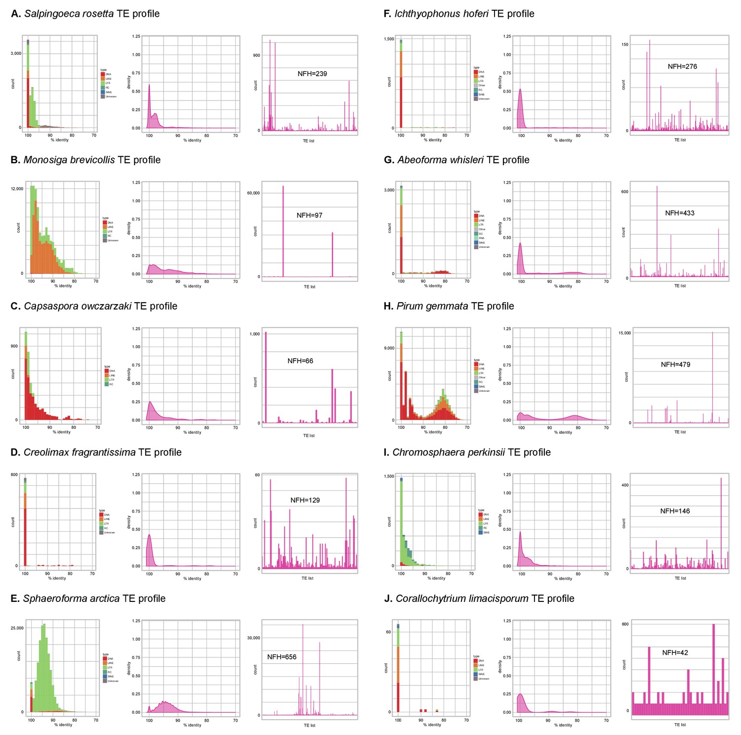
Profile of TE composition of unicellular Holozoa.
(A-J) Profile of transposable element (TE) composition of 10 unicellular Holozoa, including (i) distribution of sequence similarity frequencies within the TE complement obtained from BLAST alignments (minimum 70% identity and 80 bp alignment length); (ii) same data but using density-normalized plots; and (iii) raw counts of hits for each TE family, indicating the number of families with hits (NFH) for each species. Each third panel illustrates how TE complements can be biased towards a handful of families with a high number of similarity hits (e.g. Monosiga or Pirum) or, conversely, exhibit even distributions (e.g. Corallochytrium).
Figure 3—figure supplement 2
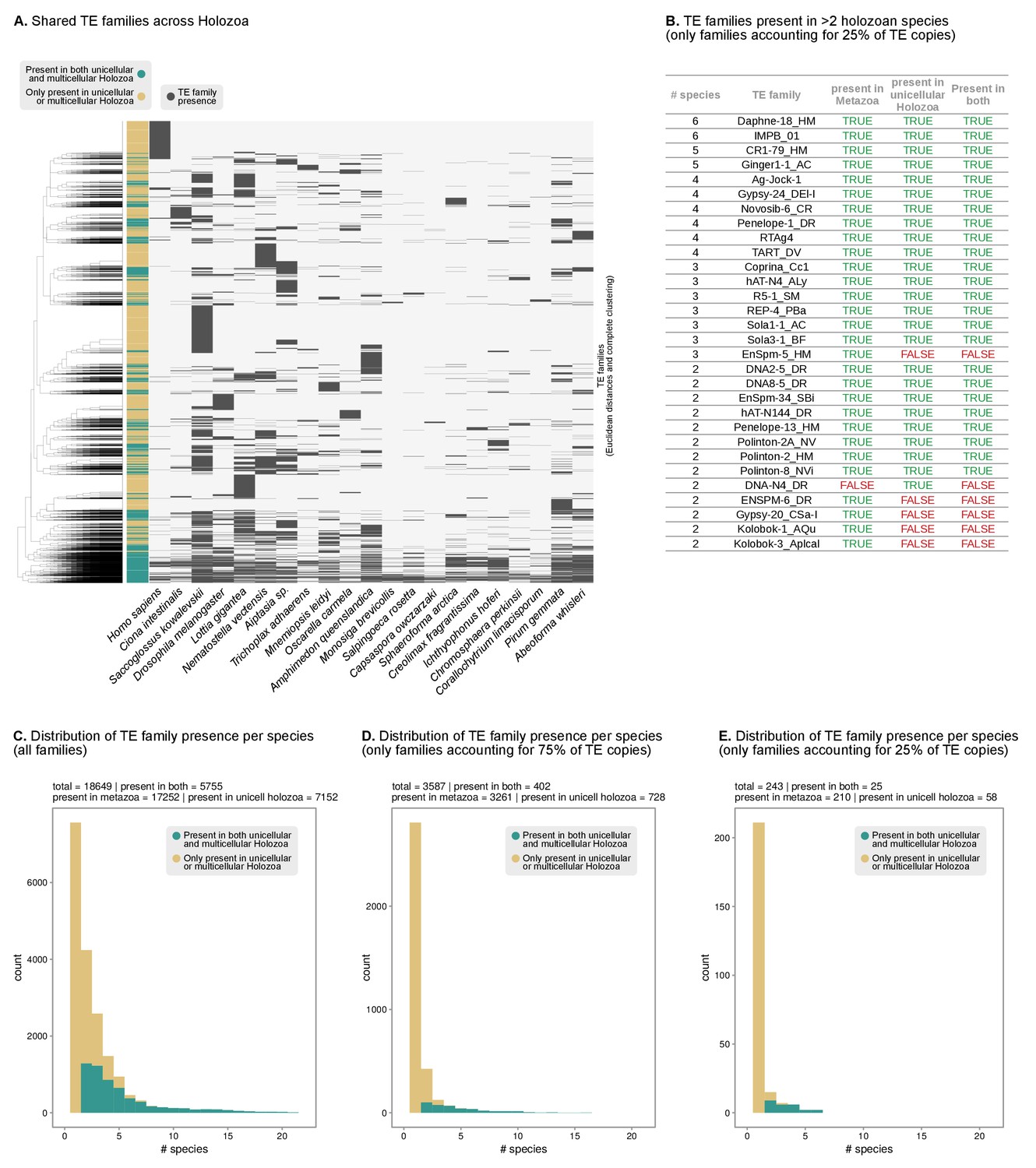
Shared TEs between unicellular Holozoa and animal genomes.
(A) Pattern of presence/absence of TE families across Holozoa (11 animals and 10 unicellular holozoans). Dendrogram at the left represents the sorting of TE families by Euclidean distance and Ward clustering. Colored column indicates presence in both unicellular and multicellular holozoans (green) or just on unicellular or multicellular holozoans (light brown). (B) List of the most abundant TE families across holozoans, including only most abundant families present in >1 species and accounting for 25% of the copies in a given genome. Complete table in Figure 3—source data 3. (C–E) Distribution of the number of TE families present in unicellular holozoans per number of species (X axis). The color code indicates presence in both unicellular and multicellular holozoans (green) or just on unicellular or multicellular holozoans (light brown). Panel C includes all TE families; panel D only most abundant TEs accounting for 75% of the copies in a given genome (P75f); panel E id. for 25% of copies (P25f).
Figure 3—figure supplement 3
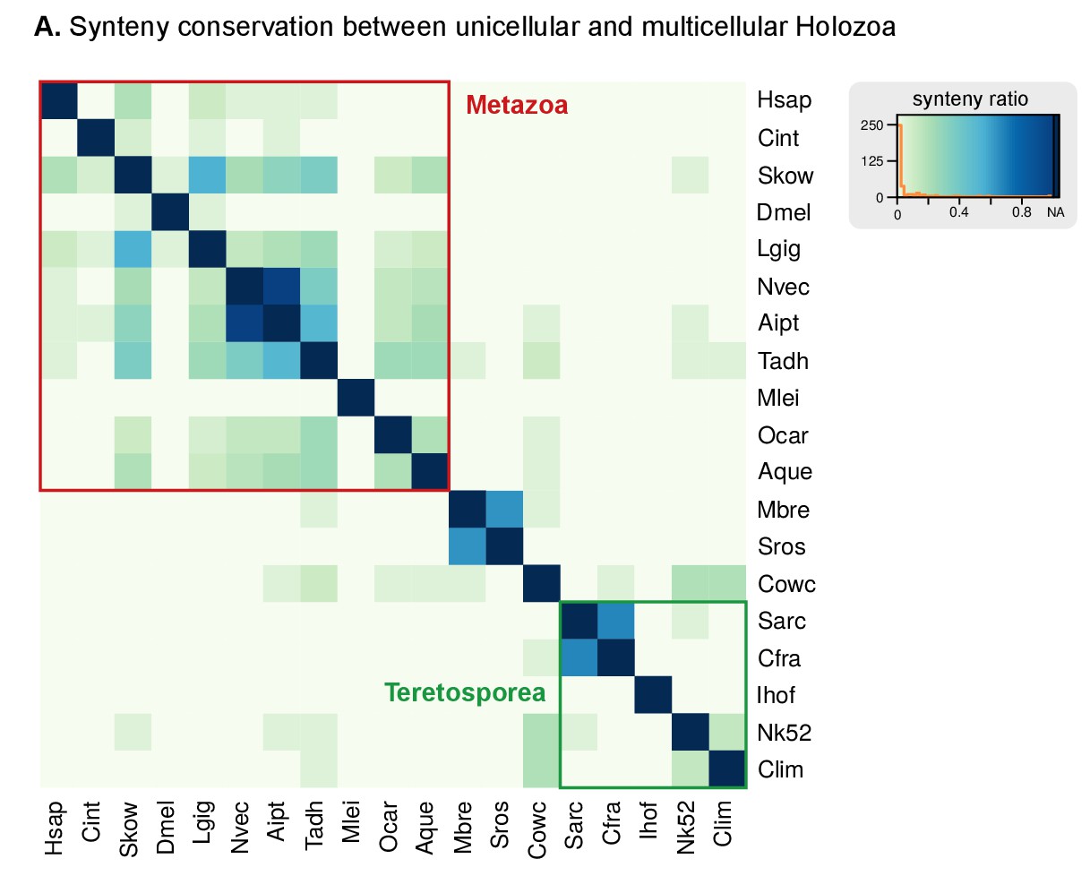
Heatmap of pairwise ratios of ortholog collinearity between 10 unicellular holozoan genomes.
Species are manually ordered by taxonomic classification (no clustering).
Figure 4
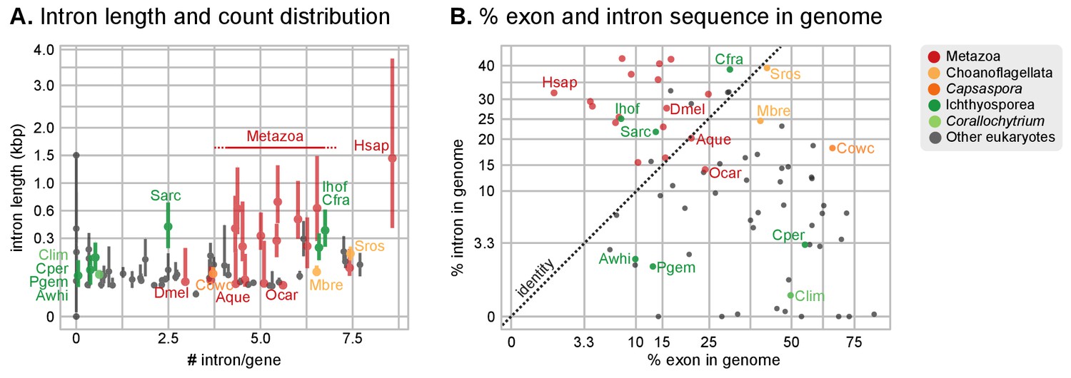
Intron abundance in eukaryotes.
(A) Distribution of intron lengths and number of introns per gene in selected eukaryote genomes. Dots represent median intron lengths and vertical lines delimit the first and third quartiles. Color code denotes taxonomic assignment. Species abbreviation as in Figure 1 and Figure 2—source data 1. (B) Fraction of the genome covered by introns and exons in selected eukaryotes. Dotted line represents the identity between both values. Color code denotes taxonomic assignment. Figure 1—source data 1.
Figure 5 with 3 supplements
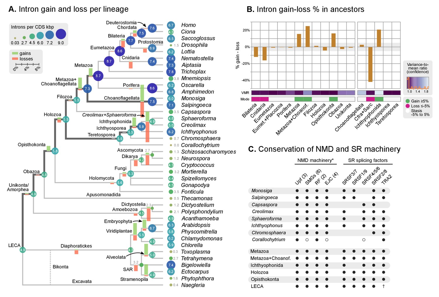
Intron evolution.
(A) Rates of intron gain and loss per lineage, including extant genomes and ancestral reconstructed nodes. Diameter and color of circles denote the number of introns per kbp of coding sequence at each ancestral node. Bolder edges mark the lines of descent between the LECA and Metazoa/Ichthyophonida, which were characterized by continued high intron densities (see text). Red and green bars represent the inferred number of intron gains (green) and losses (red) in ancestral nodes. (B) Difference between intron site gains and losses in selected ancestors, including animals (left; from Metazoa to Unikonta/Amorphea) and unicellular holozoans (right). For each ancestor, we specify the variance-to-mean ratio of the inferred number of introns from 100 bootstrap replicates (higher values, denoted by lighter purple, indicate less reliable inferences; see Methods. The color code denotes modes of intron evolution: dominance of gains (green), losses (pink) and stasis (light gray). (C) Conservation of the NMD machinery and SR splicing factors in unicellular holozoans (up) and selected ancestors (down). Black dots indicate the presence of an ortholog, and empty dots partial conservation. For the NMD machinery, each column summarizes the presence of multiple gene families (number between brackets). † denotes the ancestral eukaryotic origin of TRA2 according to (Plass et al., 2008). Complete survey at the species and gene levels available as Figure 4—figure supplements 2 and 3. Figure 5—source data 1, 2 and 3.
-
Figure 5—source data 1
Rates of gain and loss of intron sites for extant and ancestral eukaryotes, calculated for a rates-across-sites Markov model for intron evolution with branch-specific gain and loss rates (Csurös, 2008).
Used in Figure 5.
- https://doi.org/10.7554/eLife.26036.019
-
Figure 5—source data 2
Reconstruction of intron site evolutionary histories, using a rates-across-sites Markov model for intron evolution, with branch-specific gain and loss rates (Csurös, 2008).
- https://doi.org/10.7554/eLife.26036.020
-
Figure 5—source data 3
Reconstruction of the evolution of the NMD machinery (He and Jacobson, 2015) and key SR splicing factors (Plass et al., 2008).
Used in Figure 5.
- https://doi.org/10.7554/eLife.26036.021
Figure 5—figure supplement 1
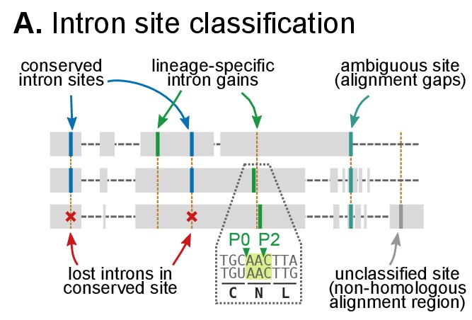
Classification of intron sites by conservation in protein alignments, as used in (Csűrös and Miklós, 2006; Csurös, 2008).
Grey boxes denote aligned amino acids with gaps (dashed lines). Intron sites (vertical lines) are conserved if they are present in various organisms at the same alignment position and codon phase. The method accounts for loss of intron sites (red crosses), independent gains at the same site (different codon phases), ambiguous sites (in poorly-aligned regions) and unclassifiable sites (non-homologous regions).
Figure 5—figure supplement 2
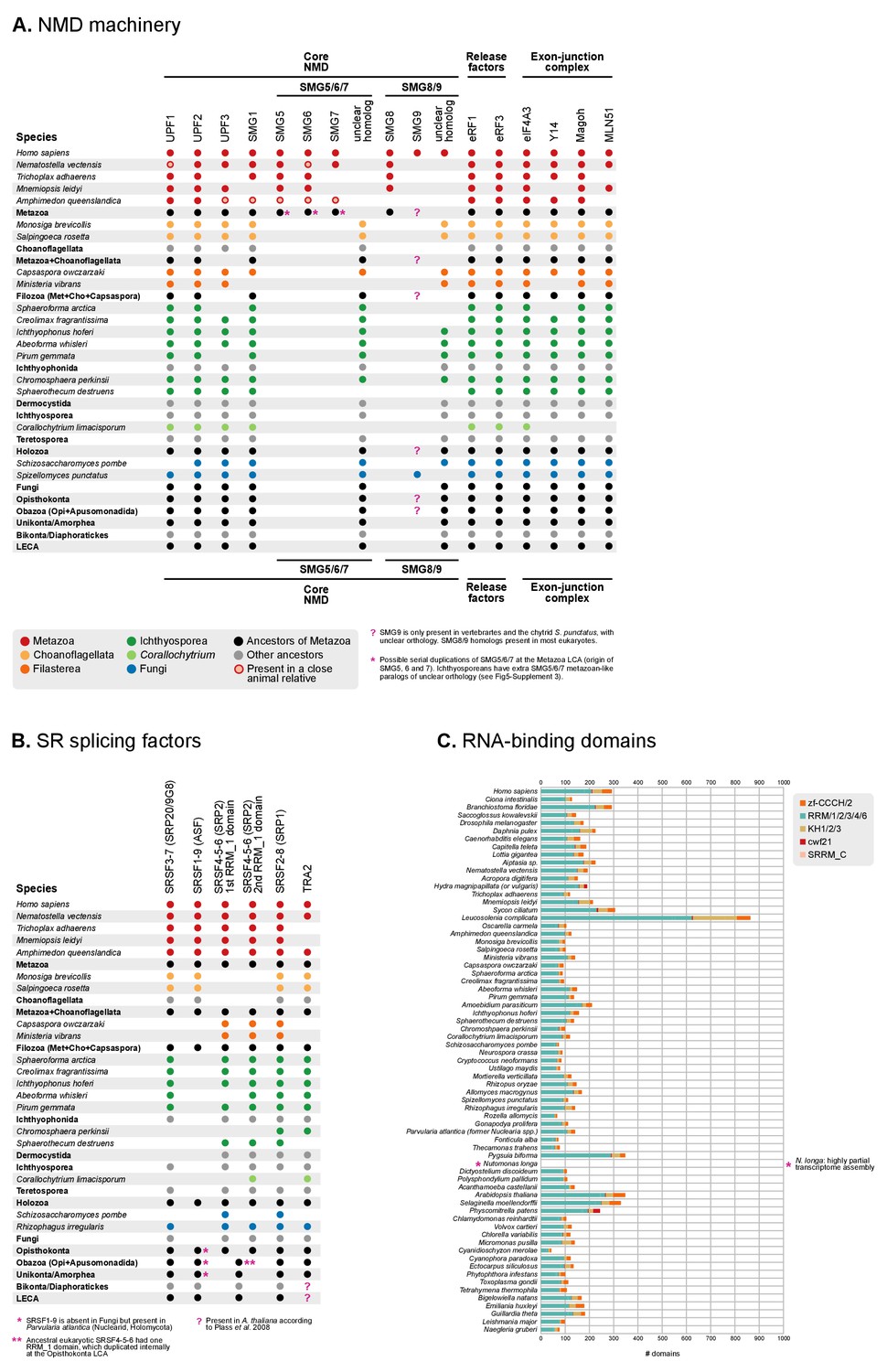
Phylogenetic distribution of the NMD machinery, SR splicing factors and RNA-binding domains in eukaryotes.
(A) Phylogenetic distribution of the NMD molecular toolkit across eukaryotes, as defined in Whelan et al. (2015), with a focus on unicellular holozoans and selected metazoans. The analysis includes 12 gene families: the core regulatory factors Upf1, Upf2 and Upf3 (also Smg2-4); the accessory proteins Smg1, Smg5/6/7 and Smg8/9; the release factors eRF1 and eRF3; and the exon junction complex (EJC) proteins eIF4A3, Y14, Magoh and MLN51. Extant species are color-coded by taxonomic assignment. Black dots indicate reconstructed LCAs within the line of descent between Metazoa and the LECA, whereas gray dots indicate LCAs not affiliated with Metaoza. Red, hollow circles indicate that a specific gene is absent from a given animal genome, but nevertheless present in a close relative in the same lineage (e.g., poriferans other than Amphimedon). See Methods for details on ortholog identification. Complete survey at the species level available as Figure 5—source data 3. Note that the core NMD tool-kit is conserved in most post-LECA LCAs, both in the animal and ichthyophonid ancestry. Secondary losses affect extant taxa: Corallochytrium lacks the complete EJC (only eIF4A3 is conserved) and homologs of Smg5/6/7 and Smg8/9. (B) Phylogenetic distribution of the SR splicing factors involved in alternative splicing determination across eukaryotes, as defined in Plass et al. (2008), with a focus on unicellular holozoans and selected metazoans. The analysis is focused on the following RNA-binding genes: SRP20/9G8 (human paralogs SRSF3/7), ASF (human paralogs SRSF1/9), SRP2 (human paralogs SRSF4/5/6), SRP1 (human paralogs SRSF2/8) and TRA2 (human paralogs TRA2A/B). Extant species are color-coded by taxonomic assignment. Black dots indicate reconstructed LCAs within the line of descent between Metazoa and the LECA, whereas gray dots indicate LCAs not affiliated with Metaoza. See Methods for details on ortholog identification. Complete survey at the species level available as Figure 5—source data 3. Note that the complement of SR genes is conserved in most post-LECA LCAs, including Opisthokonta, Holozoa and Metazoa. Secondary losses are, however, frequent in some lineages: SRSF1/9 is lost in Fungi, Teretosporea and Filasterea; Corallochytrium lacks all canonical SR genes but TRA2 and a fragmentary SRSF4/5/6; choanoflagellates have lost SRSF4/5/6, etc. (C) Counts of RNA-binding protein domains in extant eukaryotic genomes. Unicellular holozoans have a rich complement of RNA-binding proteins (domains per species: average 127.8; median 120), albeit less abundant than metazoans’ (domains per species: average 225.3; median 187).
Figure 5—figure supplement 3
Phylogenetic analysis of (A) eIF4A3, (B) Smg5/6/7, and (C) eRF3, using Maximum likelihood in IQ-TREE (supports are SH-like approximate likelihood ratio test/UFBS, respectively); including Bayesian inference supports for the ortologous groups of interest (BPP statistical supports, in red).
https://doi.org/10.7554/eLife.26036.024
Figure 6
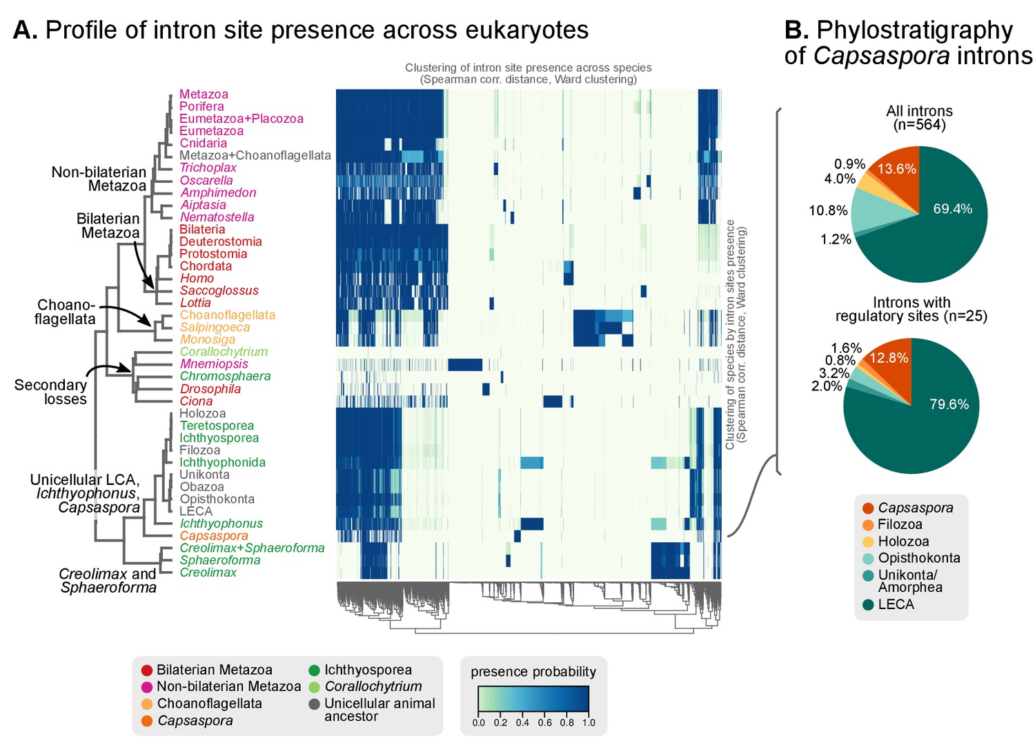
Profile of intron site presence across eukaryotes.
(A) Heatmap representing presence/absence of 4312 intron sites (columns) from extant and ancestral holozoan genomes, plus the line of ascent to the LECA (rows). Intron sites and genomes have been grouped according to their respective patterns of co-occurrence (dendrogram based on Spearman correlation distances and Ward clustering algorithm; see Methods). The dendrogram of genome clusterings is shown to the left. Figure 5—source data 2. (B) Phylostratigraphic analysis of the origin of Capsaspora introns, considering all sites (left) and those with putative regulatory sites (right; after [Sebé-Pedrós et al., 2016b]).
Figure 7 with 1 supplement
Evolution of protein domain architectures.
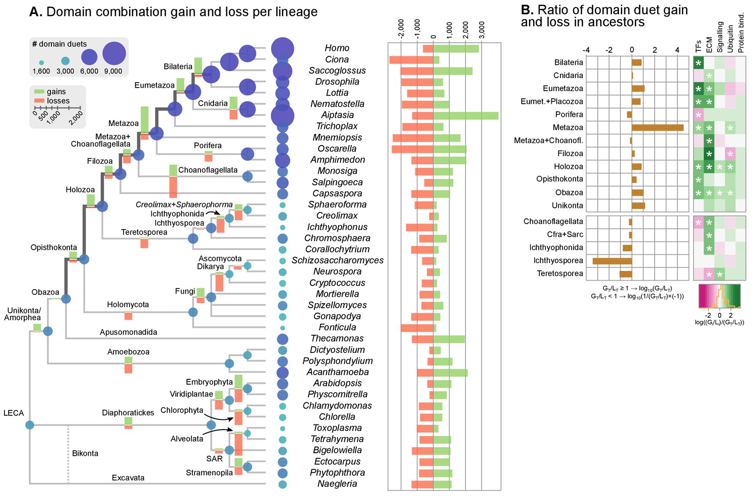
(A) Protein domain combination gain and loss per lineage, including extant genomes and ancestral reconstructed nodes. Diameter and color of circles denote the number of different domain combinations (in different gene families) in that node of the tree. Bolder edges mark the line of descent between the LCAs of Opisthokonta and Bilateria, which was generally dominated by gains of protein domain combinations (see text). Red and green bars represent the inferred number of gains and losses, respectively. (B) Gain/loss ratio of protein domain diversity in selected ancestors, including animals (upper chart; from Metazoa to Unikonta/Amorphea) and unicellular holozoans (lower). Heatmap to the right represents the log-ratio value of the diversification rate for selected sub-sets of functionally-related protein domains relevant to multicellularity: green indicates higher-than-average diversification; pink less; white asterisks indicate two-fold or more increases or decreases (all comparisons relative to the whole set of protein domains). Source Data Figure 7—source data 1, 2, 3 and 4.
-
Figure 7—source data 1
Rates of gain and loss of protein domain pairs within a given orthogroup for extant and ancestral eukaryotes, calculated for a phylogenetic birth-and-death probabilistic model that accounts for gains, losses and duplications (Csurös, 2010).
- https://doi.org/10.7554/eLife.26036.027
-
Figure 7—source data 2
Reconstruction of the evolutionary histories of protein domain pairs gains within orthogroups, using a phylogenetic birth-and-death probabilistic model that accounts for gains, losses and duplications (Csurös, 2010).
- https://doi.org/10.7554/eLife.26036.028
-
Figure 7—source data 3
Reconstruction of the evolutionary histories of individual protein domains, using Dollo parsimony and accounting for gains and losses (Csurös, 2010).
- https://doi.org/10.7554/eLife.26036.029
-
Figure 7—source data 4
Rates of gain and loss of orthogroups for extant and ancestral eukaryotes, using a phylogenetic birth-and-death probabilistic model that accounts for gains, losses and duplications.
Used in Figures 1.
- https://doi.org/10.7554/eLife.26036.030
Figure 7—figure supplement 1
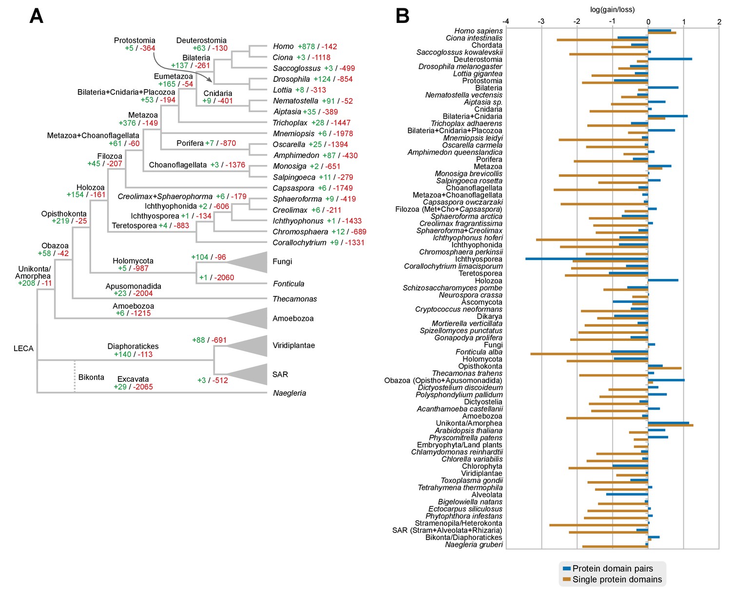
Gains and losses of individual protein domains across eukaryotes.
(A) Ancestral reconstruction of gains (green) and losses (red) of protein domains per lineage, based on Dollo parsimony. Note that, in contrast with the evolution of protein domain combinations here most nodes are dominated by losses. The most notable exceptions are the Metazoa and Opisthokonta LCAs (dominated by gains) and its unicellular ancestors from Holozoa to Choanoflagellata + Metazoa LCAs (in which gains and losses are in a relative stasis). Figure 7—source data 3. (B) Log-ratio of gains-to-losses for single protein domains (brown bars) and protein domain pairs (blue bars), based on the respective ancestral reconstructions. Positive values thus mean that gains are greater than losses. Loss of single protein domains dominates in most nodes, but gains in protein domain combinations can nevertheless outweigh losses in many ancestors (e.g., Holozoa or Metazoa LCAs).
Figure 8 with 1 supplement
Protein domain architecture networks.
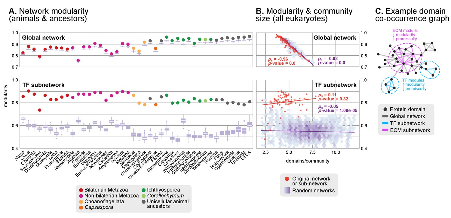
(A and B) Modularity and community size of the global network of domain pairs (upper panels) and the TF subnetwork (lower panels), with ≥90% probability. The modularity parameter measures the fraction of the intra-community edges in the network, minus the expected value in a random network (takes values from 0 to 1; see Materials and methods and [Newman and Girvan, 2004]). Panels at the left show the observed modularity of the protein domain (sub)networks of various genomes (Holozoa and selected ancestors; dots are taxa-colored). Purple box plots represent the distribution of simulated modularities from 100 rewirings of the original organism-specific networks, while keeping a constant vertex degree distribution. Panels to the right show the relationship between modularities and the number of domains/community, both for actual genomes (orange) and simulated rewired networks (purple density plot, see Methods). Monotonic dependence between modularity and domains/community was tested for each set of data (global, TF and their respective simulations) using Spearman's rank correlation coefficient (ρs), and linear regression fits are included for clarity. Note that simulated TF subnetworks are less modular and have more domains/community than the original ones, signaling their higher-than-expected modularities. Note that the scales of the vertical axes change between upper and lower panels. (C) Example of protein domain co-occurrence network. Vertices represent domains, linked by edges if they co-occur within the same gene family. Two subnetworks are highlighted in yellow (domain pairs occurring in TF genes) or green (same for signaling genes). Figure 7—source data 1 and 2, Figure 1—source data 2.
Figure 8—figure supplement 1
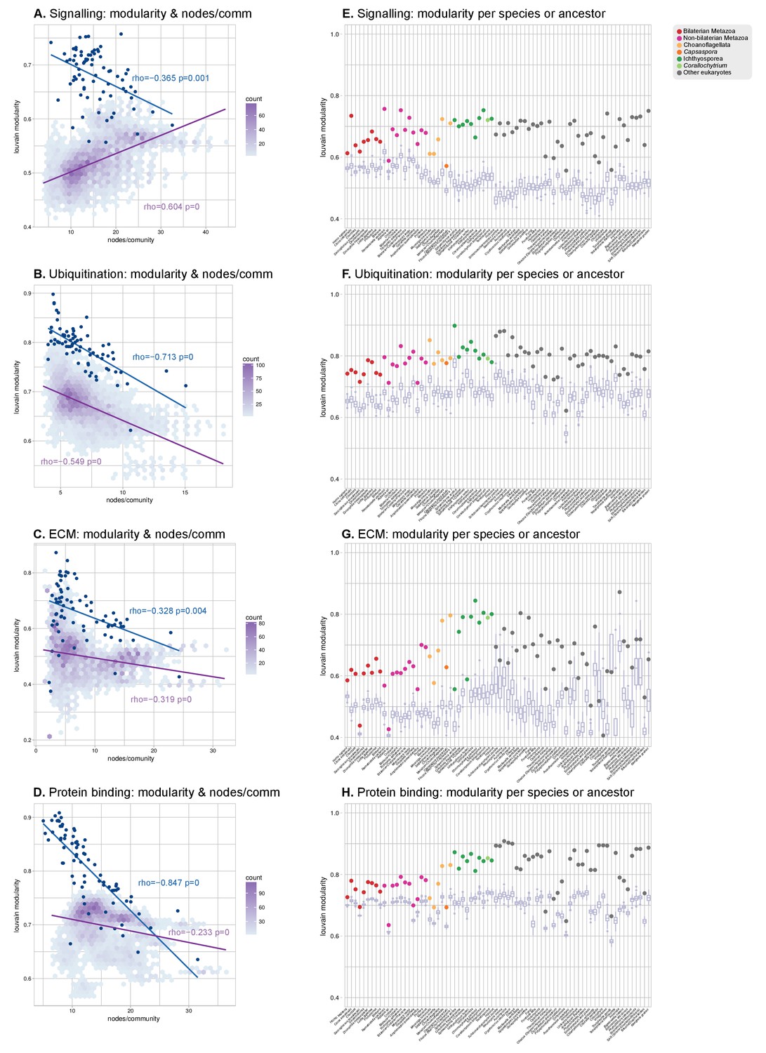
Modularity of protein domain co-occurrence networks of multicellularity-related gene sets across eukaryotes.
(A–D) Modularity and community size of the functional sub-networks based on domains related to signaling (Richter and King, 2013), ubiquitination (Grau-Bové et al., 2015), ECM (Richter and King, 2013; Sebé-Pedrós et al., 2010; Hynes, 2012) and protein binding (Mitchell et al., 2015) functions. Blue dots indicate real genomes, and the purple density plot indicates the values of the simulated rewired networks. Monotonic dependence between modularity and domains/community was tested for each set of data using Spearman's rank correlation coefficient (ρs); linear regression fits are included for clarity. All sub-networks (A–D) have the same decreasing trend as the global sub-network of Figure 8A–B, and contrast with the results for TFs. (E–H) Modularity of the functional sub-network based on domains related to signaling, ubiquitination, ECM and protein binding functions (same domains as in A-D), per species or ancestral node (colored dots). Purple box plots represent the distribution of simulated modularities from 100 rewirings of the original organism-specific networks, while keeping a constant vertex degree distribution. Note the decreased modularities shown by metazoans (red and pink) in all sub-networks.
Figure 9 with 1 supplement
Phylogenetic analysis of the premetazoan gene families LIM Homeobox, CBP/p300 and type IV collagen.
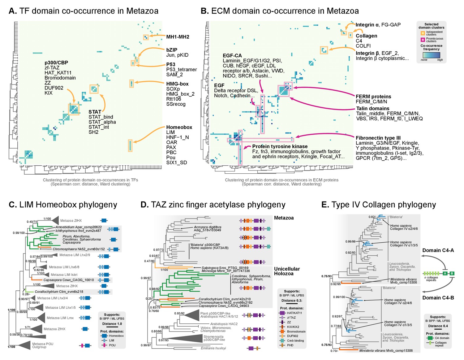
(A and B) Protein domain co-occurrence matrices of transcription factor (TF) (A) or extracellular matrix (ECM)-related gene families (B), inferred at the LCA of Metazoa (≥90% probability). Horizontal and vertical axes of the heatmap represent individual protein domains and their mutual co-occurrence frequency, and have been clustered according to the number of shared domains (dendrogram based on Spearman correlation distances and Ward clustering algorithm). Note that, for TFs, most co-occurrence clusters are located along the diagonal, indicating isolated domain communities; whereas ECM genes tend to contain promiscuous domains shared in multiple domain co-occurrence communities. Representative examples of independent and promiscuous domain clusters have been highlighted in both heat maps (orange and pink, respectively). (C) Phylogenetic tree of LIM Homeobox TFs, with mapped protein domains architectures. (D) Phylogenetic tree of CBP/p300 TFs based on HAT/KAT11 domain, with mapped consensus protein domain architectures. (E) Phylogeny of type IV collagen genes based on the C4 domain. All extant homologs, from Ministeria to animals, have a C4-C4 dual arrangement of filozoan origin (reflected in the phylogeny by two parallel clades representing the first and second domains within each gene). Ministeria (orange) and human (blue) homologs are highlighted. In C, D and E panels, bold branches represent unicellular holozoan genes and are color-coded by taxonomic assignment. All trees are Bayesian inferences (BI). Protein domain architectures and statistical supports (BPP/UFBS) are shown for selected nodes (see Figure 9—figure supplement 1 for the complete BI and ML trees with statistical supports). Figure 7—source data 1 and 2.
Figure 9—figure supplement 1
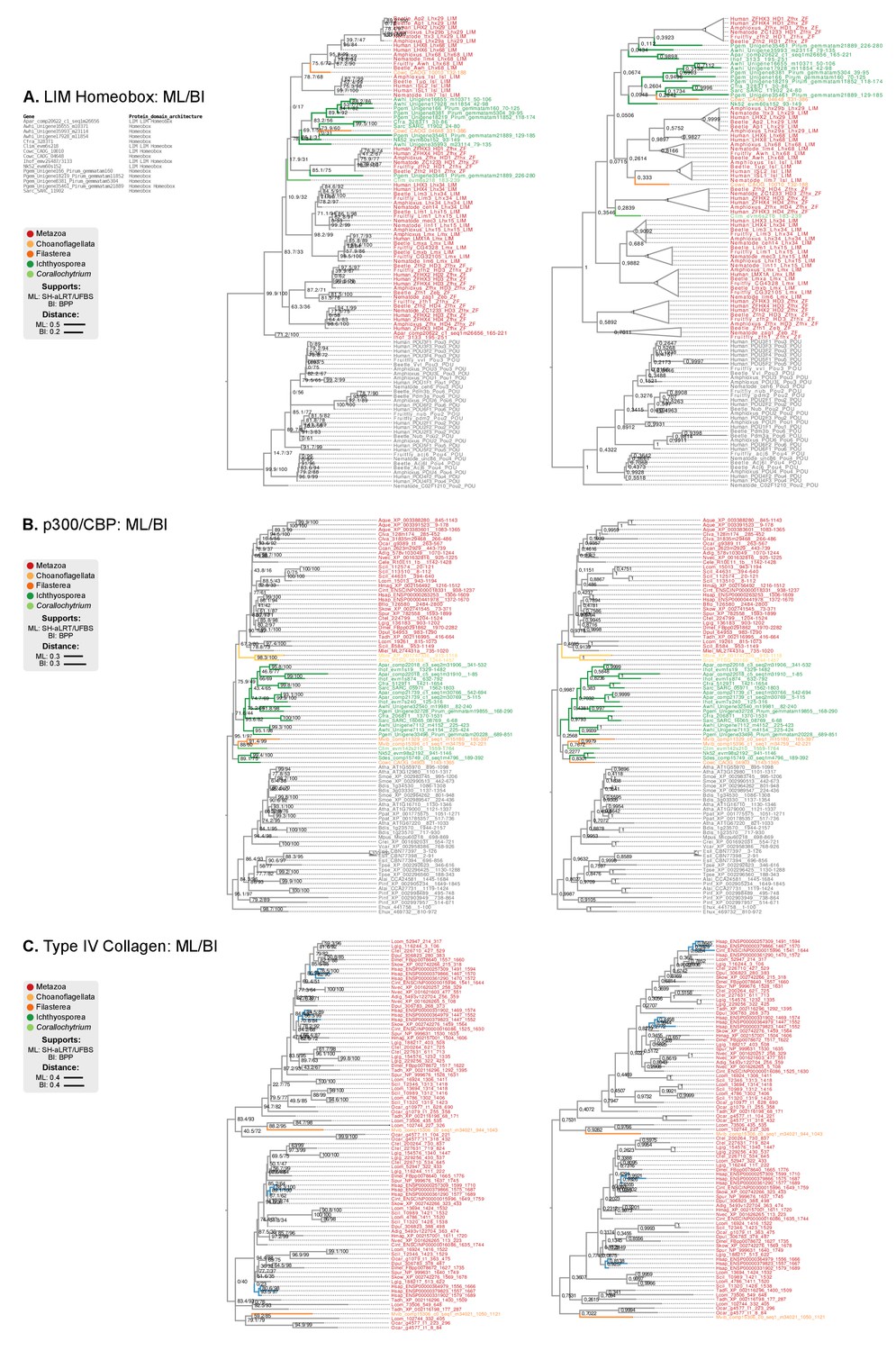
Phylogenetic analysis of the (A) LIM-Homeobox, (B) p300/CBP, and (C) Collagen Type IV, using Maximum likelihood in IQ-TREE (supports are SH-like approximate likelihood ratio test/UFBS, respectively) and Bayesian inference in Mr. Bayes (BPP statistical supports).
https://doi.org/10.7554/eLife.26036.035
Figure 10
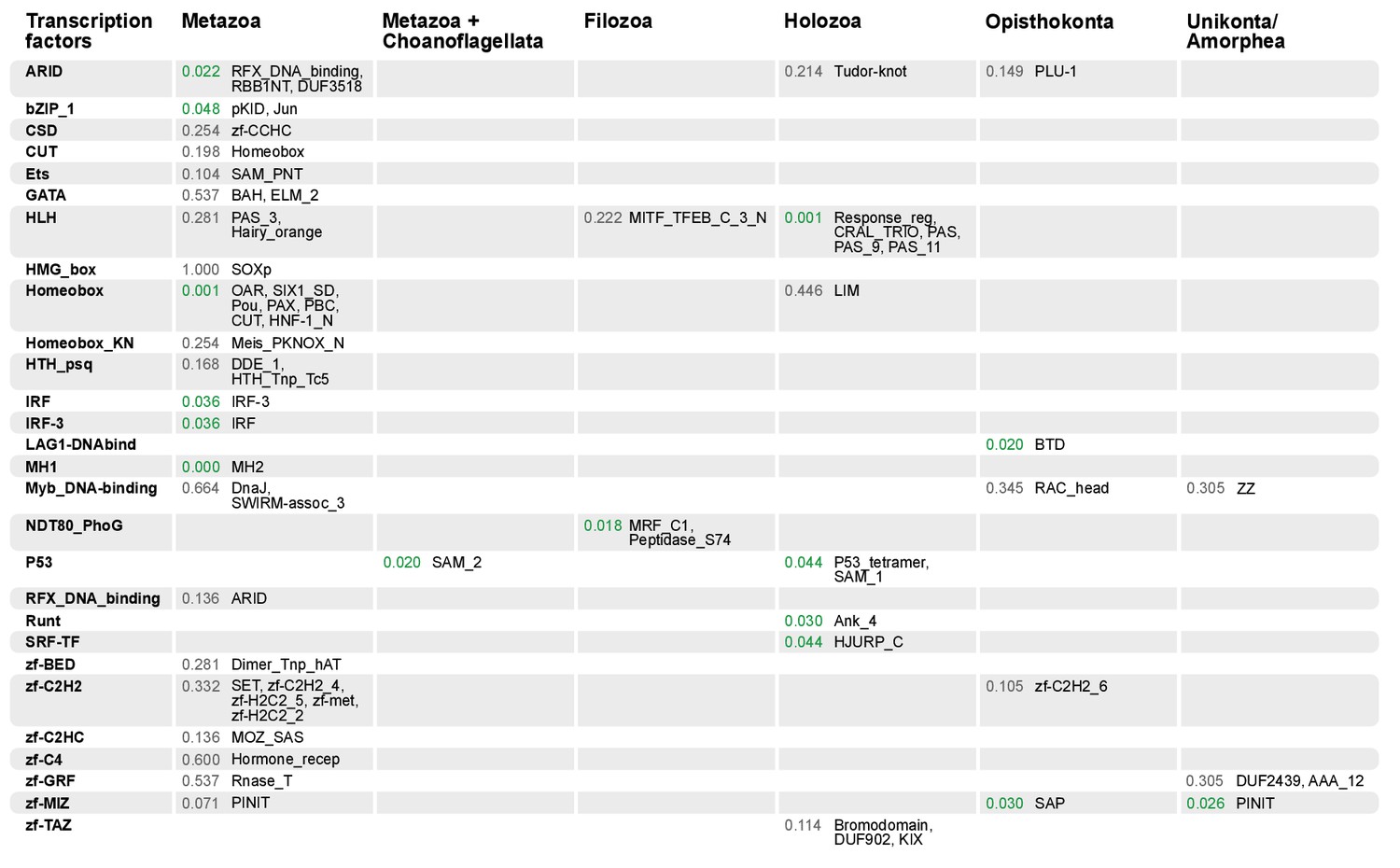
Domain combinations that appear in transcription factor (TF) families in unicellular premetazoans, from the LCA of Unikonta/Amorphea to the LCA of Metazoa.
First and second columns indicate the TF family and its inferred evolutionary origin, respectively (from [de Mendoza et al., 2013]). Subsequent columns list (i) the p-value of a Fisher's exact test for the relative enrichment of that TF family in that node of the tree (compared to other domains that rearrange there; p-values<0.05 in green); and (ii) the accessory domains that appear within each TF family. Figure 7—source data 2, Table 1.
-
Figure 10—source data 1
Probability of emergence of protein domain combinations present in the LCA of Metazoa in previous ancestral nodes (from LCA of Metazoa to LCA of Unikonta/Amorphea).
Only protein domain combinations with >90% presence probability in the LCA of Metazoa were included. Protein domain combinations that are not gained with >90% probability in any of the surveyed nodes have been associated with LECA or pre-LECA origins (‘1’ values in the ‘LECA or before’ field). Used in Figure 10.
- https://doi.org/10.7554/eLife.26036.037
Download links
A two-part list of links to download the article, or parts of the article, in various formats.
Downloads (link to download the article as PDF)
Open citations (links to open the citations from this article in various online reference manager services)
Cite this article (links to download the citations from this article in formats compatible with various reference manager tools)
Dynamics of genomic innovation in the unicellular ancestry of animals
eLife 6:e26036.
https://doi.org/10.7554/eLife.26036


