A quantitative approach for analyzing the spatio-temporal distribution of 3D intracellular events in fluorescence microscopy
- Inria, Centre Rennes-Bretagne Atlantique, France
- PSL Research University, Institut Curie, France
- IBiSA, Institut Curie, France
Figures
Figure 1
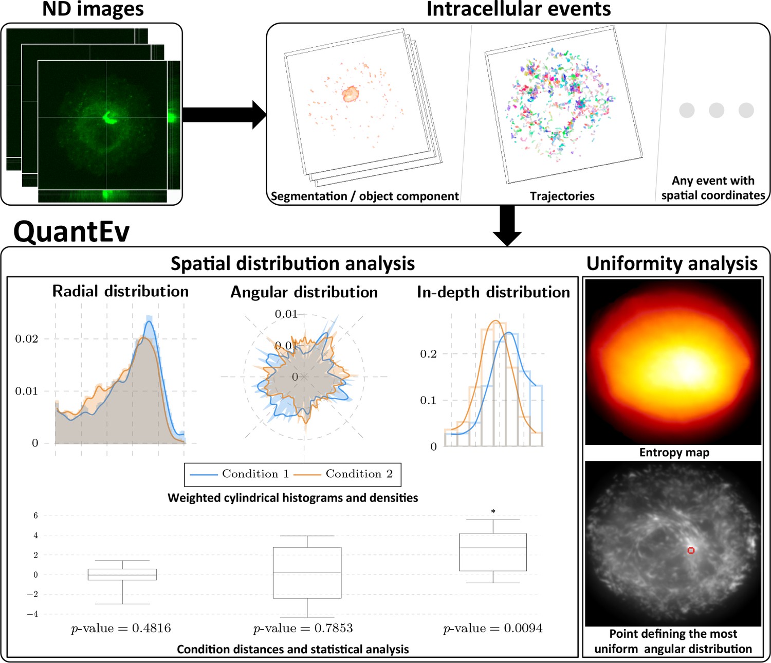
Overview of QuantEv approach.
Spatial distribution analysis: QuantEv computes 3D histograms and densities of intracellular descriptors to quantitatively compare different experimental conditions. Uniformity analysis: QuantEv identifies the point that gives the most uniform angular distribution of intracellular descriptors.
Figure 2

Spatial distribution analysis of Rab6 proteins.
(a−c) 3D KD maps obtained with kernel density maps when considering all image sequences with unconstrained (a), crossbow- (b) and disk- (c) shaped cells. (d) Box and whisker plots of the p values obtained when comparing randomly 100 times two groups of unconstrained (UCC), crossbow-shaped (CSC) or disk-shaped cells (DSC) with QuantEv and KD maps. (e) Box and whisker plots of the condition differences with respect to radius , angle and depth over 58 image sequences. p values under conditions of one-sided Wilcoxon signed-rank test when considering the condition differences are indicated below the box and whisker plots. A star (*) indicates that the p value is smaller than 0.05. (f) Histograms (bar plots) and densities (lines) of the spatial distribution of Rab6 positive membranes with respect to radius , angle and depth . These distributions come from 18 image sequences with an unconstrained cell (blue bar plots and lines), 18 image sequences with a crossbow-shaped cell (orange bar plots and lines) and 22 image sequences with a disk-shaped cell (green bar plots and lines). (g−i) Overlay of the average intensity projection map of an image sequence with an unconstrained (g), crossbow- (h) and disk- (i) shaped cell and the radial levels at 0.6 and 0.8. The scale bars correspond to 5 m.
Figure 3

Spatial distribution analysis of moving Rab6 proteins.
(a–c) Rab6 trajectories moving toward the cell periphery (red trajectories) and toward Golgi (green trajectories) extracted from an image sequence with an unconstrained (a), a crossbow- (b) and a disk- (c) shaped cell. The scale bars correspond to 5 m. (d-f) Histograms (bar plots) and densities (lines) of the spatial distribution of Rab6-positive membranes moving toward the cell periphery (green bar plots and lines) or toward the Golgi (pink bar plots and lines) with respect to radius , angle and depth . These distributions come from 18 image sequences with an unconstrained cell (d), 18 image sequences with a crossbow-shaped cell (e) and 22 image sequences with a disk-shaped cell (f). The box and whisker plots of the condition differences of the spatial distribution of moving Rab6-positive membranes with respect to radius , angle and depth for unconstrained (d), crossbow- (e) and disk- (f) shaped cells are next to the histograms and densities. p values under conditions of one-sided Wilcoxon signed-rank test when considering the condition differences are indicated below the box and whisker plots. A star (*) indicates that the p value is smaller than 0.05.
Figure 4
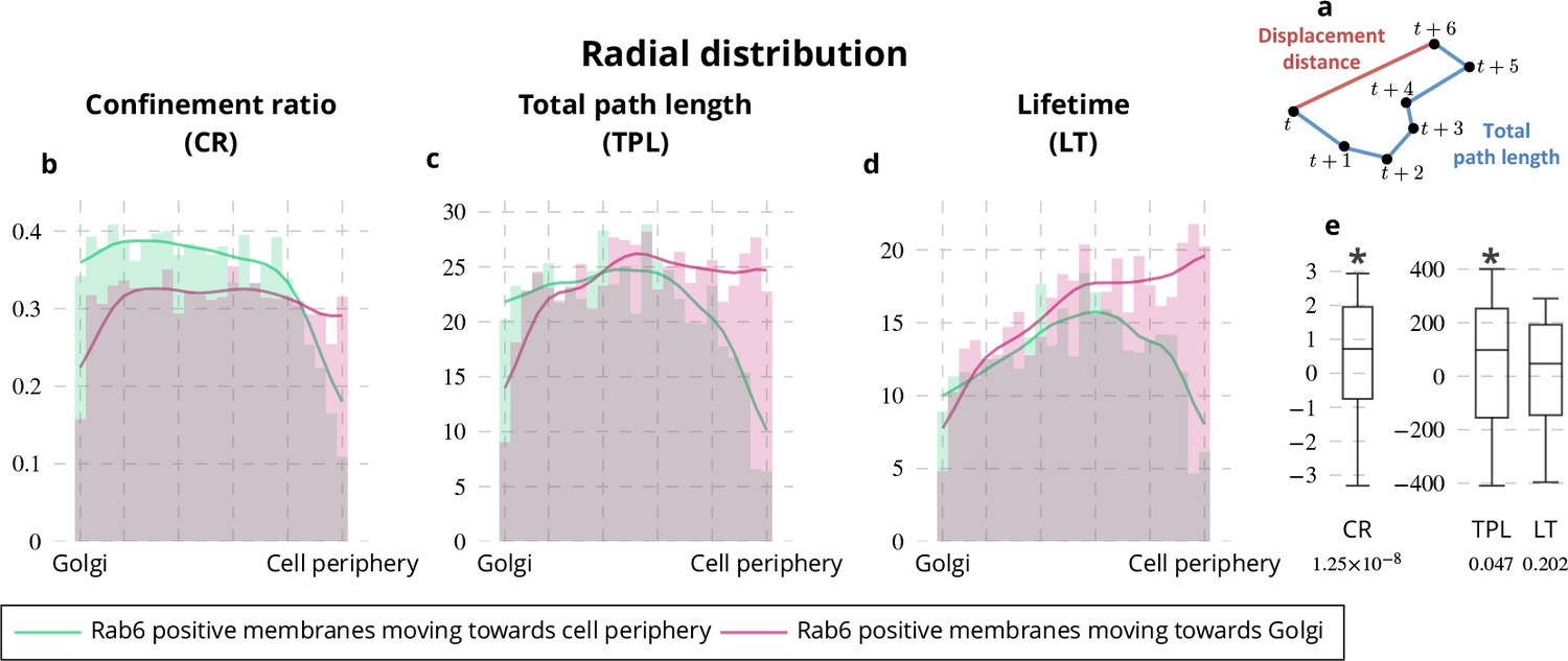
Radial distribution of Rab6 dynamic features.
(a) Illustration of the displacement distance and the total path length of a trajectory. The confinement ratio is defined as the ratio between the displacement distance and the total path length. (b-d) Histograms (bar plots) and densities (lines) showing the radial distribution of confinement ratio (b), total path length (c) and lifetime (d) for trajectories of Rab6-positive membranes. These distributions come from the grouping of 18 image sequences with unconstrained cells, 18 image sequences with crossbow-shaped cells and 22 image sequences with disk-shaped cells. (e) Box and whisker plots showing the condition differences of the radial distribution of confinement ratio (CR), total path length (TPL) and lifetime (LT) for trajectories of Rab6-positive membranes. p values under conditions of one-sided Wilcoxon signed-rank test when considering the condition differences are indicated below the box and whisker plots. A star (*) indicates that the p value is smaller than 0.05.
Figure 5
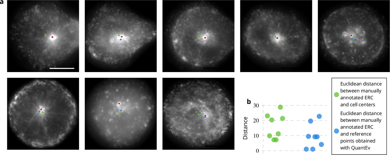
Estimation of the endosomal recycling center (ERC) location from the angular distribution of Rab11-positive membranes.
(a) The red disks correspond to the manual annotation, the blue disks to the point defining the most uniform angular distribution of Rab11-positive membranes and the green disks correspond to the cell centers. These disks are displayed over the average intensity projections of the image sequences showing Rab11-positive membranes. The scale bar corresponds to 5 m. (b) Euclidean distances between the manually annotated ERC and the cell centers (green disks) or the points giving the most uniform angular distribution (blue disks).
Figure 6
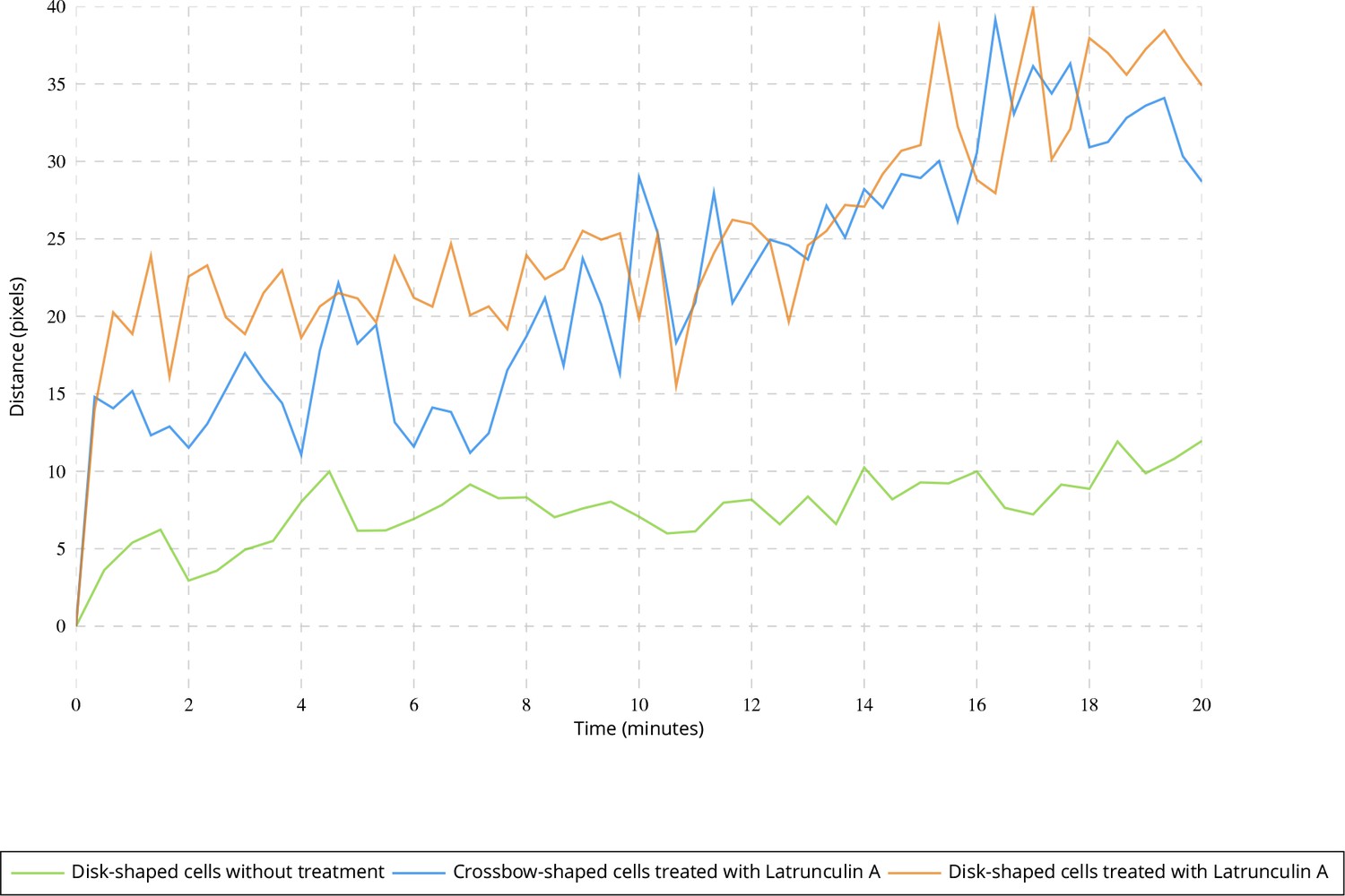
Evolution of the point giving the most uniform angular distribution over time.
Average Euclidean distance between the point giving the most uniform distribution at time t = 0 and the point estimated at further frames for untreated disk-shaped cells (four image sequences) and cells treated with Latrunculin A (six image sequences for each micro-pattern).
Figure 7
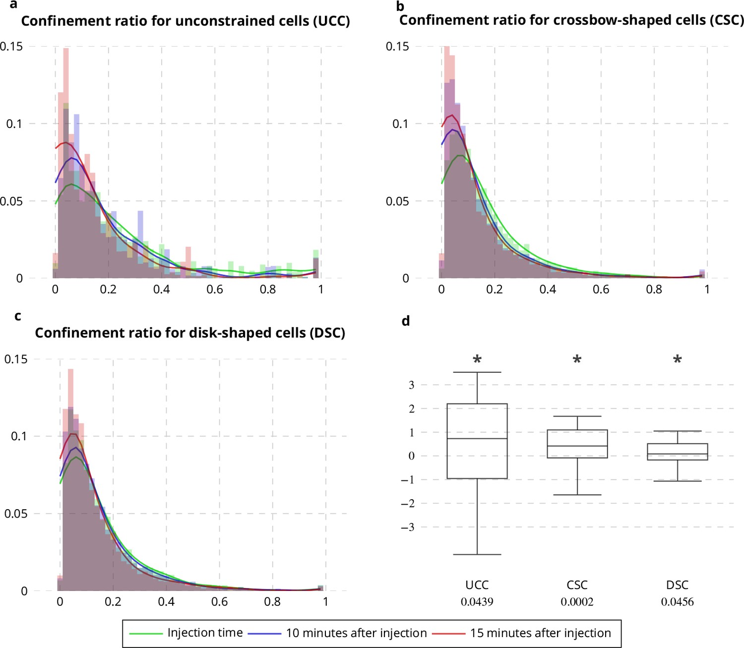
Confinement ratio of Rab11-positive membranes with Latrunculin A injection.
(a-c) Histograms (bar plots) and densities (lines) of the confinement ratio of Rab11 positive membranes on unconstrained (a), crossbow- (b) and disk- (c) shaped cells at Latrunculin A Injection Time, 10 and 15 min after injection. (d) Box and whisker plots of the corresponding condition differences (five image sequences for unconstrained cells, 10 image sequences for crossbow-shaped cells and nine image sequences for disk-shaped cells). p values under conditions of one-sided Wilcoxon signed-rank test when considering the condition differences are indicated below the box and whisker plots. A star (*) indicates that the p value is smaller than 0.05.
Figure 8
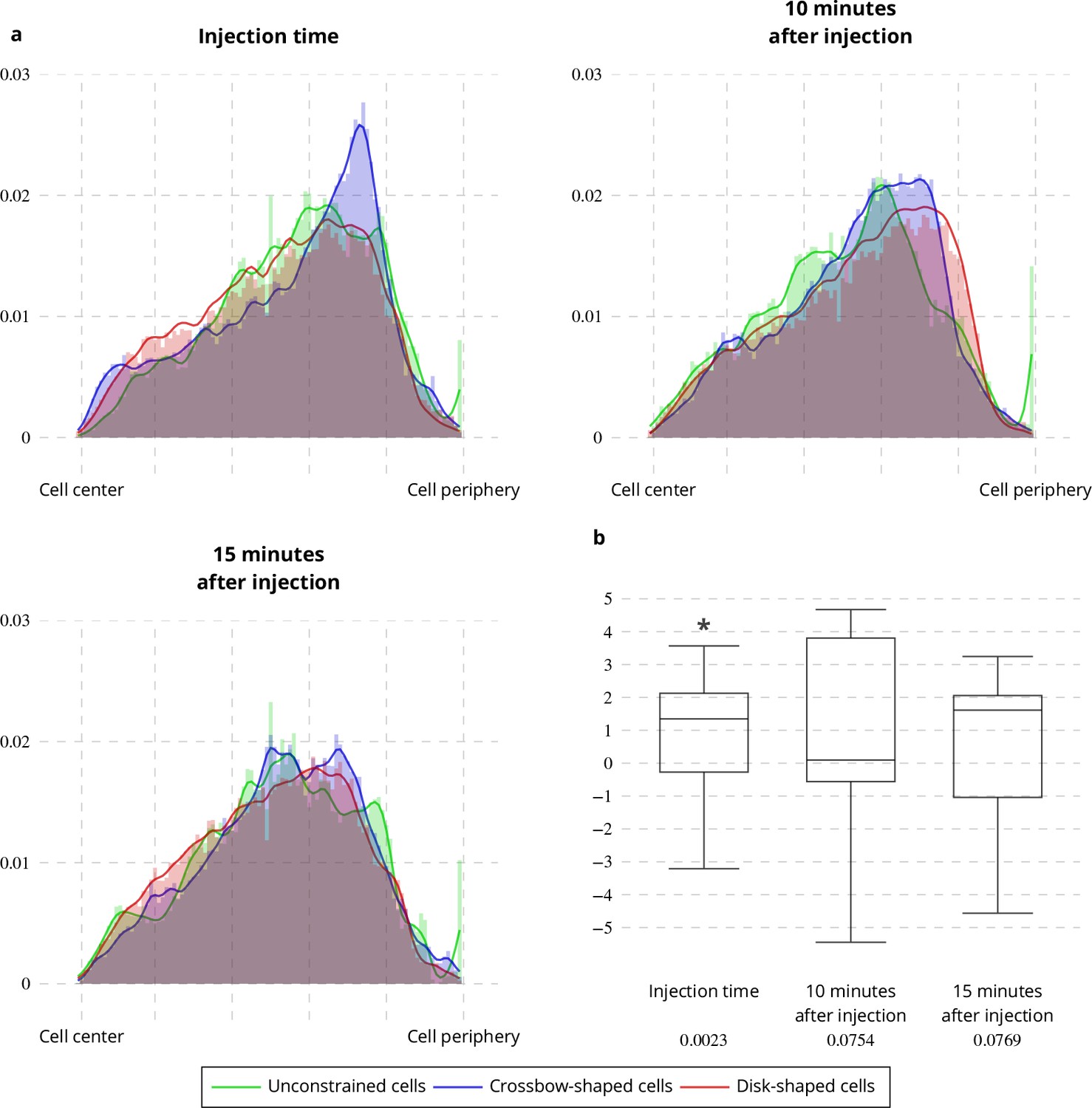
Latrunculin A influence on Rab11 radial distribution.
(a) Histograms (bar plots) and densities (lines) of the radial distribution of Rab11-positive membranes on unconstrained, crossbow- and disk-shaped cells at Latrunculin A Injection Time, 10 and 15 min after injection. (b) Box and whisker plots of the condition differences of the radial distribution between unconstrained, crossbow- and disk-shaped cells at Latrunculin A Injection Time, 10 and 15 min after injection. p values under conditions of one-sided Wilcoxon signed-rank test when comparing unconstrained, crossbow- and disk-shaped cells (five image sequences for unconstrained cells, ten image sequences for crossbow-shaped cells and nine image sequences for disk-shaped cells) are indicated below the box and whisker plots.
Appendix 1—figure 1
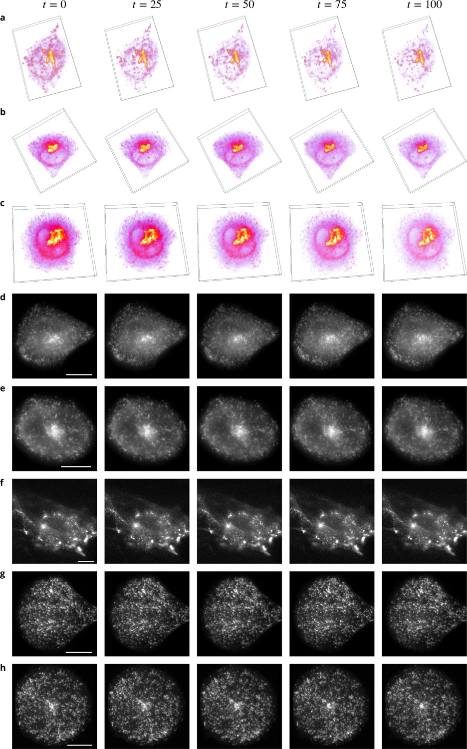
Example images from the datasets.
(a-c) Volume renderings of fluorescent images taken from three sequences showing Rab6 proteins in an unconstrained (a), a crossbow- (b) and a disk- (c) shaped cell. (d–e) Fluorescent images taken from two sequences showing Rab11 proteins in a crossbow- (d) and a disk- (e) shaped cell. (f–h) Fluorescent images taken from three sequences showing Rab11 proteins treated with Latrunculin A in an unconstrained (f), a crossbow- (g) and a disk- (h) shaped cell. In Figs d–h, the intensity over the planes is averaged, a gamma correction is applied for a better visualization and the scale bars correspond to 5 m.
Appendix 1—figure 2
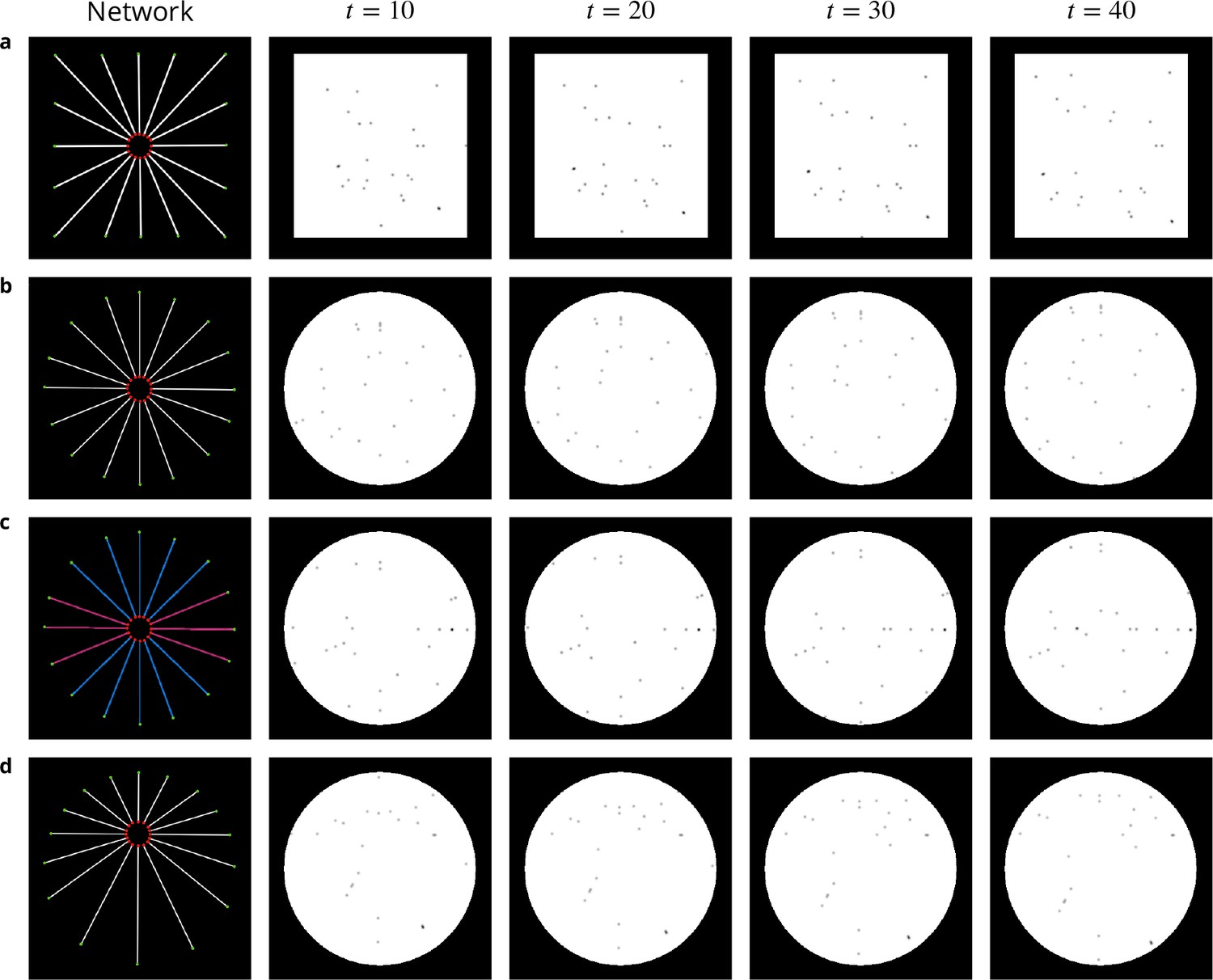
Image sequences simulated to evaluate QuantEv performance.
First column: networks used to generate four image sequences. The particle origins are labeled as red disks while particle destinations appear as green disks. Particles for the sequences a, c and d are uniformly distributed over the different paths. Particles for the sequence c are distributed with a probability equal to 0.1 over the pink paths and with a probability equal to 0.04 over the blue paths. Images corresponding to time t=10, t=20, t=30 and t=40 taken from one simulated image sequence for each network are illustrated in columns 2 to 5.
Appendix 2—figure 1
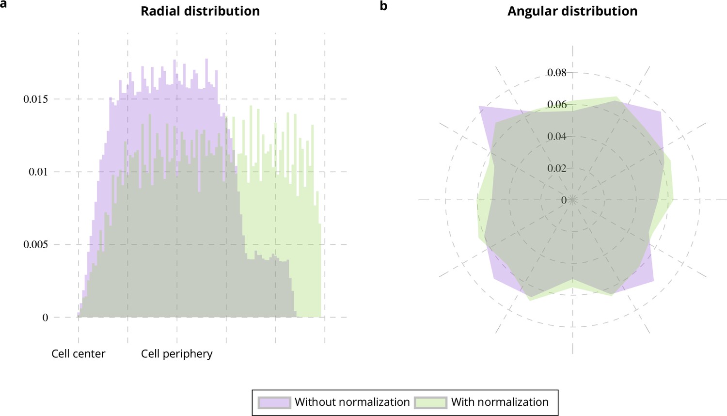
Cell shape normalization.
Radial (a) and angular (b) distributions of particles moving on square-shaped cells from 10 simulated image sequences (Appendix 1—figure 2a) with (green histograms) and without normalization (purple histograms) with respect to the distance between the cell center and the cell periphery.
Appendix 3—figure 1
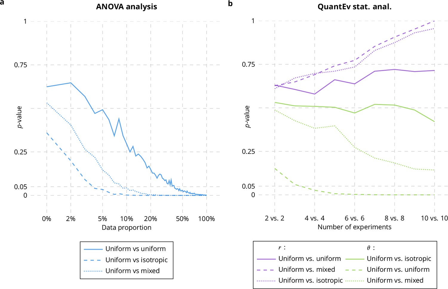
Comparison between ANOVA and QuantEv.
p-values obtained with ANOVA statistical analysis (a) and QuantEv statistical analysis (b) when considering the spatial distribution of particles uniformly distributed (Appendix 1—figure 2b), isotropically distributed (Appendix 1—figure 2c) and a mix of uniformly and isotropically distributed particles over 16 paths.
Appendix 4—figure 1
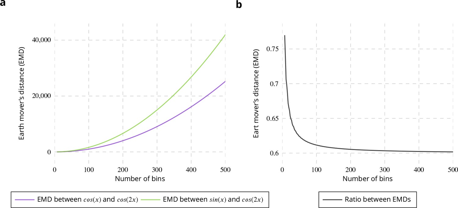
Evaluation of binning influence on earth mover’s distance.
(a) Earth Mover’s Distance (EMD) between and (purple curve) and between and (green curve). (b) Ratio between the two EMDs shown on left plot.
Appendix 6—figure 1
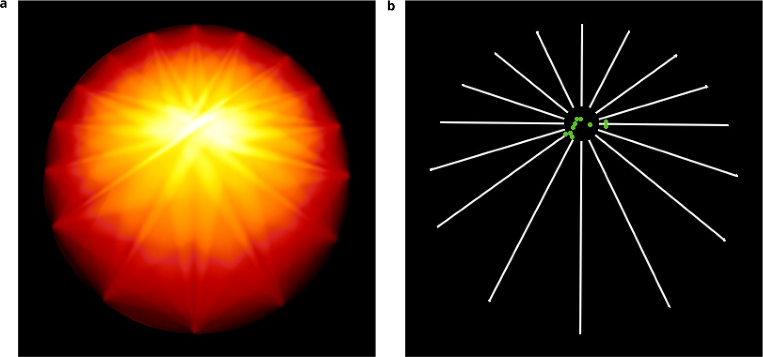
Uniformity analysis.
(a) Entropy map obtained on a simulated image sequence (see Appendix 1—figure 2d) showing at each point the angular distribution entropy obtained when considering this point as the reference. (b) Estimated reference points (green disks) obtained for 10 different simulated image sequences.
Videos
Appendix 1—figure 1—video 1
Rab6 proteins in an unconstrained cell.
Volume rendering of fluorescent images showing Rab6 proteins in an unconstrained cell corresponding to Appendix 1—figure 1a.
Appendix 1—figure 1—video 2
Rab6 proteins in a crossbow-shaped cell.
Volume rendering of fluorescent images showing Rab6 proteins in a crossbow-shaped cell corresponding to Appendix 1—figure 1b.
Appendix 1—figure 1—video 3
Rab6 proteins in a disk-shaped cell.
Volume rendering of fluorescent images showing Rab6 proteins in a disk-shaped cell corresponding to Appendix 1—figure 1c.
Appendix 1—figure 1—video 4
Rab11 proteins in a crossbow-shaped cell.
Image sequence showing Rab11 proteins in a crossbow-shaped cell corresponding to Appendix 1—figure 1d.
Appendix 1—figure 1—video 5
Rab11 proteins in a disk-shaped cell.
Image sequence showing Rab11 proteins in a disk-shaped cell corresponding to Appendix 1—figure 1e.
Appendix 1—figure 1—video 6
Rab11 proteins treated with Latrunculin A in an unconstrained cell.
Image sequence showing Rab11 proteins treated with Latrunculin A in an unconstrained cell corresponding to Appendix 1—figure 1f.
Appendix 1—figure 1—video 7
Rab11 proteins treated with Latrunculin A in a crossbow-shaped cell.
Image sequence showing Rab11 proteins treated with Latrunculin A in a crossbow-shaped cell corresponding to Appendix 1—figure 1g.
Appendix 1—figure 1—video 8
Rab11 proteins treated with Latrunculin A in a disk-shaped cell.
Image sequence showing Rab11 proteins treated with Latrunculin A in a disk-shaped cell corresponding to Appendix 1—figure 1h.
Appendix 1—figure 2—video 1
Simulation of uniformly distributed particles in a square-shaped cell.
Image sequence simulated with particles uniformly distributed over 16 paths on a square-shaped cell, corresponding to Appendix 1—figure 2a.
Appendix 1—figure 2—video 2
Simulation of uniformly distributed particles in a disk-shaped cell.
Image sequence simulated with particles uniformly distributed over 16 paths on a disk-shaped cell, corresponding to Appendix 1—figure 2b.
Appendix 1—figure 2—video 3
Simulation of isotropically distributed particles in a disk-shaped cell.
Image sequence simulated with particles distributed over 16 paths with two different probabilites on a disk-shaped cell, corresponding to Appendix 1—figure 2c.
Appendix 1—figure 2—video 4
Simulation of uniformly distributed particles around an uncentered emitter in a disk-shaped cell.
Image sequence simulated with particles uniformly distributed over 16 paths on a disk-shaped cell, around an emitter located in the upper part of the cell, corresponding to Appendix 1—figure 2d.
Tables
Appendix 5—table 1
QuantEv processing time.
https://doi.org/10.7554/eLife.32311.034| Image size | Object | Histogram and | Point with most uniform distribution | |
|---|---|---|---|---|
| Coverage | Density computation | Bisection method | Entropy map | |
| 256 × 256 | 10% | 0.5 s | 42.1 s | 8min45s |
| 256 × 256 | 60% | 0.6 s | 2min31s | 47min16s |
| 512 × 512 | 10% | 1.6 s | 2 min 20 s | 2h11min |
| 512 × 512 | 60% | 1.7 s | 11 min 48 s | 11 hr 3 min |
Additional files
-
Transparent reporting form
- https://doi.org/10.7554/eLife.32311.011
Download links
A two-part list of links to download the article, or parts of the article, in various formats.
Downloads (link to download the article as PDF)
Open citations (links to open the citations from this article in various online reference manager services)
Cite this article (links to download the citations from this article in formats compatible with various reference manager tools)
A quantitative approach for analyzing the spatio-temporal distribution of 3D intracellular events in fluorescence microscopy
eLife 7:e32311.
https://doi.org/10.7554/eLife.32311


