Enrichment drives emergence of functional columns and improves sensory coding in the whisker map in L2/3 of mouse S1
- University of California, Berkeley, United States
Figures
Figure 1 with 1 supplement
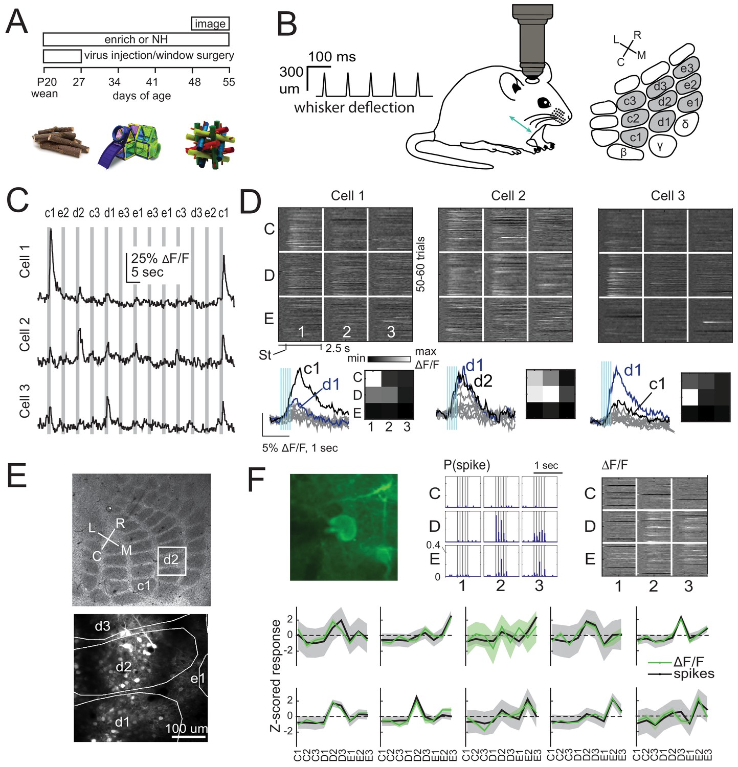
2-photon calcium imaging of whisker responses and receptive fields in S1.
(A) Experimental time line and example enrichment objects. (B) Schematic of whisker stimulus train and barrel map showing the 3 × 3 array of stimulated whiskers in gray. (C) Example ΔF/F traces from 3 ROIs imaged simultaneously in L2/3 of one column from a Drd3-Cre mouse. Gray bars are deflections of each indicated whisker. (D) Whisker receptive fields for the 3 cells in (C). Top, ΔF/F traces (shown as grayscale after baseline subtraction) for each trial for the nine whiskers (C1 to E3), aligned to stimulus onset (St). Bottom left, Mean ΔF/F trace for each whisker. Vertical bars are whisker deflections. The two strongest whiskers are shown in black and blue, respectively. Bottom right, Median ΔF/F averaged over 1 s response window. (E) Localization of one L2/3 imaging field (box) in a Drd3-Cre mouse relative to column boundaries in a cytochrome oxidase-stained section through L4 (top). Bottom, projection of barrel boundaries onto this imaging field. (F) Comparison of receptive fields measured by simultaneous GCaMP6s imaging and loose-seal cell-attached spike recording. Top: One example L2/3 neuron with its spiking receptive field shown as a peristimulus time histogram for each whisker (center), and its imaging receptive field from ΔF/F (right). Bottom: Average imaging and spiking receptive fields for each whisker-responsive neuron (n = 10). Shading is SEM.
Figure 1—figure supplement 1
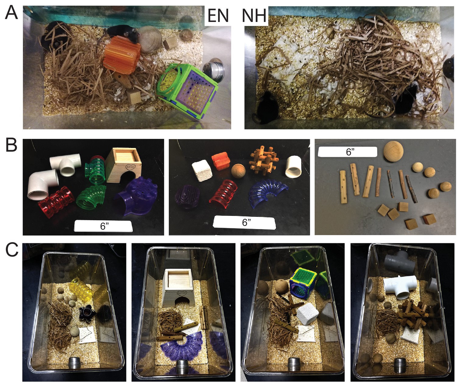
Home-cage enrichment paradigm.
(A) Example enriched cage containing three mice, toys, nesting material and bedding (EN) and normally housed cage containing two mice, nesting material and bedding (NH). Overhead food and water dispensers, and cage lid, were present in all cages but are not shown here for clarity. (B) Examples of the three types of enrichment toys: burrow-type toys (left), medium-sized toys (middle), and small wooden toys (right). Scale bars are six inches. (B) Examples of toy combinations used in enrichment cages. Each EN cage contained one burrowing toy, one medium-sized toy, and several small wooden toys.
Figure 2 with 2 supplements
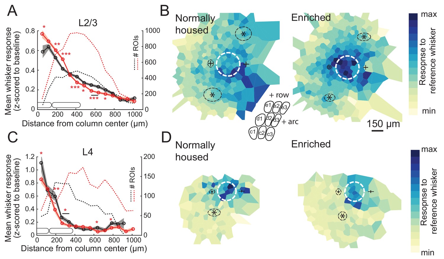
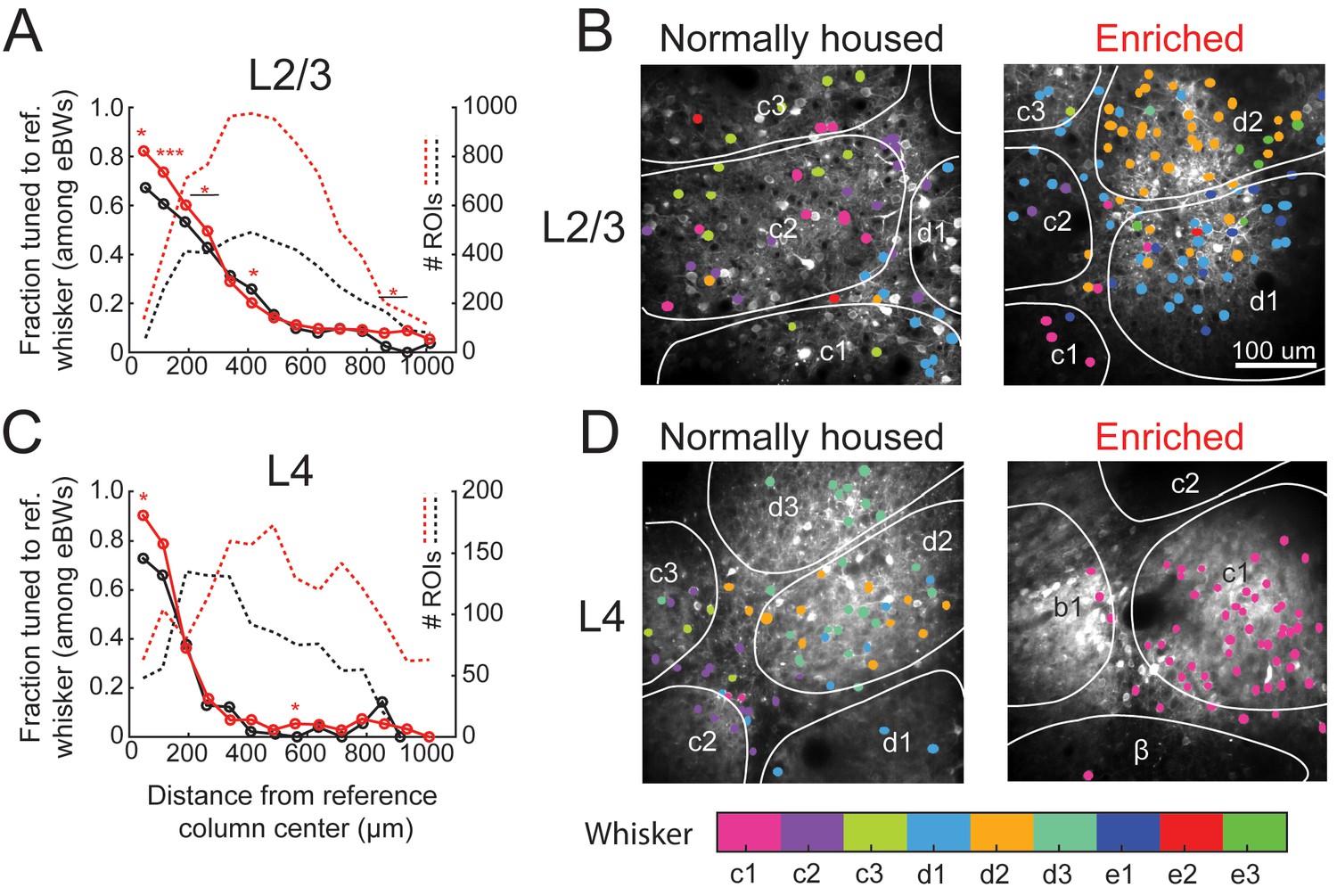
Enrichment strengthens and sharpens the whisker point representation in L2/3.
(A) Average evoked response in L2/3 to a reference whisker (ΔF/F, z-scored to spontaneous activity in each cell) across all ROIs at increasing distances from the reference column center. ROIs are grouped into 75 μm width bins. Shading shows SEM. (B) Mean 2D spatial distribution of evoked responses to a reference whisker in L2/3. Dashed white circle is the reference whisker’s column (shown as average barrel diameter around column center). All whisker-responsive ROIs within 750 μm of each reference column, across all imaging fields, are included. Color indicates mean response in each bin. Individual imaging fields were centered on the reference column and rotated to align the within-row anatomical axis horizontally. Pluses show mean location of column centers for within-arc, row+one and within-arc, row-1 whiskers. Stars show mean location of column centers for within-row, arc-1 and within-row, arc+one whiskers. Dashed black ellipses indicate standard deviation of these column centroids. Inset: schematic of barrel field in the same orientation as plots. (C–D) Same as A-B, but for L4 ROIs in Scnn1a-Cre mice.
Figure 2—figure supplement 1
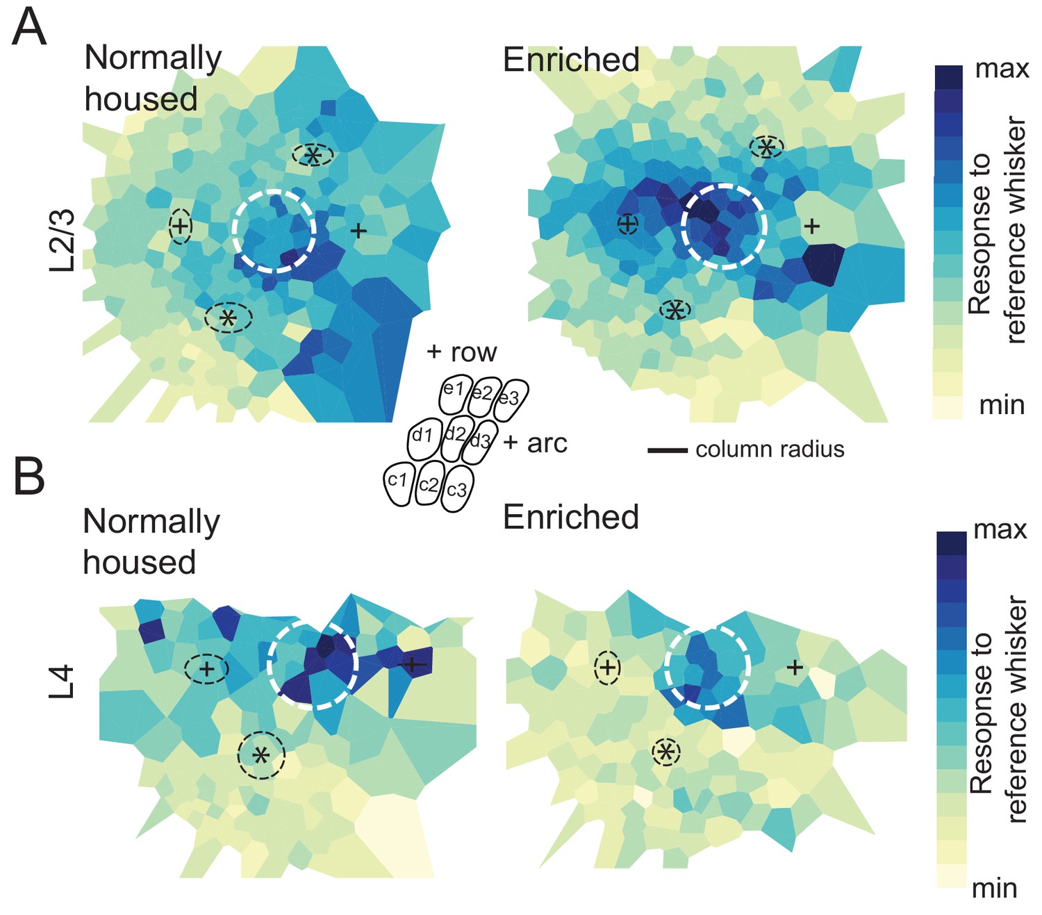
Whisker point representation analyzed in a column-based reference frame.
(A) Mean 2D spatial distribution of evoked responses to a reference whisker for ROIs around that whisker’s column. For this figure, the distance from each ROI to the reference column center was normalized to the radius of the reference column along the vector connecting the ROI to the column center. Thus, distance is in units of reference column radius. Dashed white circle represents the precise border of the reference column. All whisker-responsive L2/3 ROIs within 5 radii of the reference column center are included. Other plotting conventions are as in Figure 2. (B) Whisker point representation in L4, plotted as in (A).
Figure 2—figure supplement 2
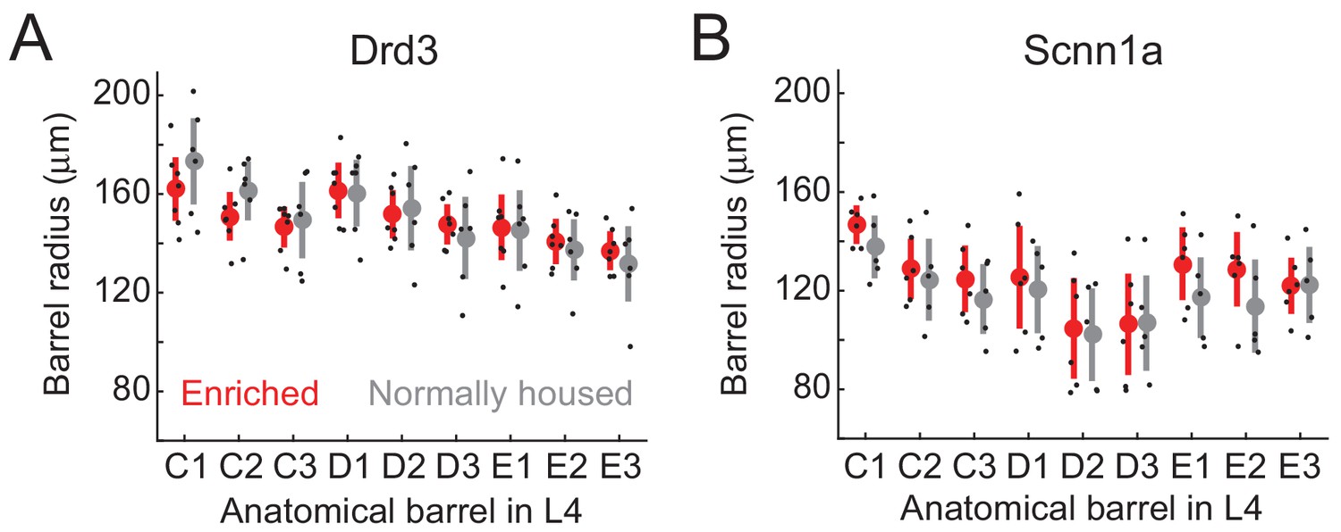
Size of L4 barrels in enriched vs. normally housed mice.
(A) Radius for each of 9 anatomical whisker barrels, in Drd3-Cre mice. Red and gray show mean ± SEM for EN and NH mice. Black dots are individual mice. (B) Same measurement for Scnn1a-Cre mice. For each panel, a 2-way ANOVA was performed with factors of enrichment and barrel identity. There was no significant enrichment effect for either genotype.
Figure 3 with 1 supplement
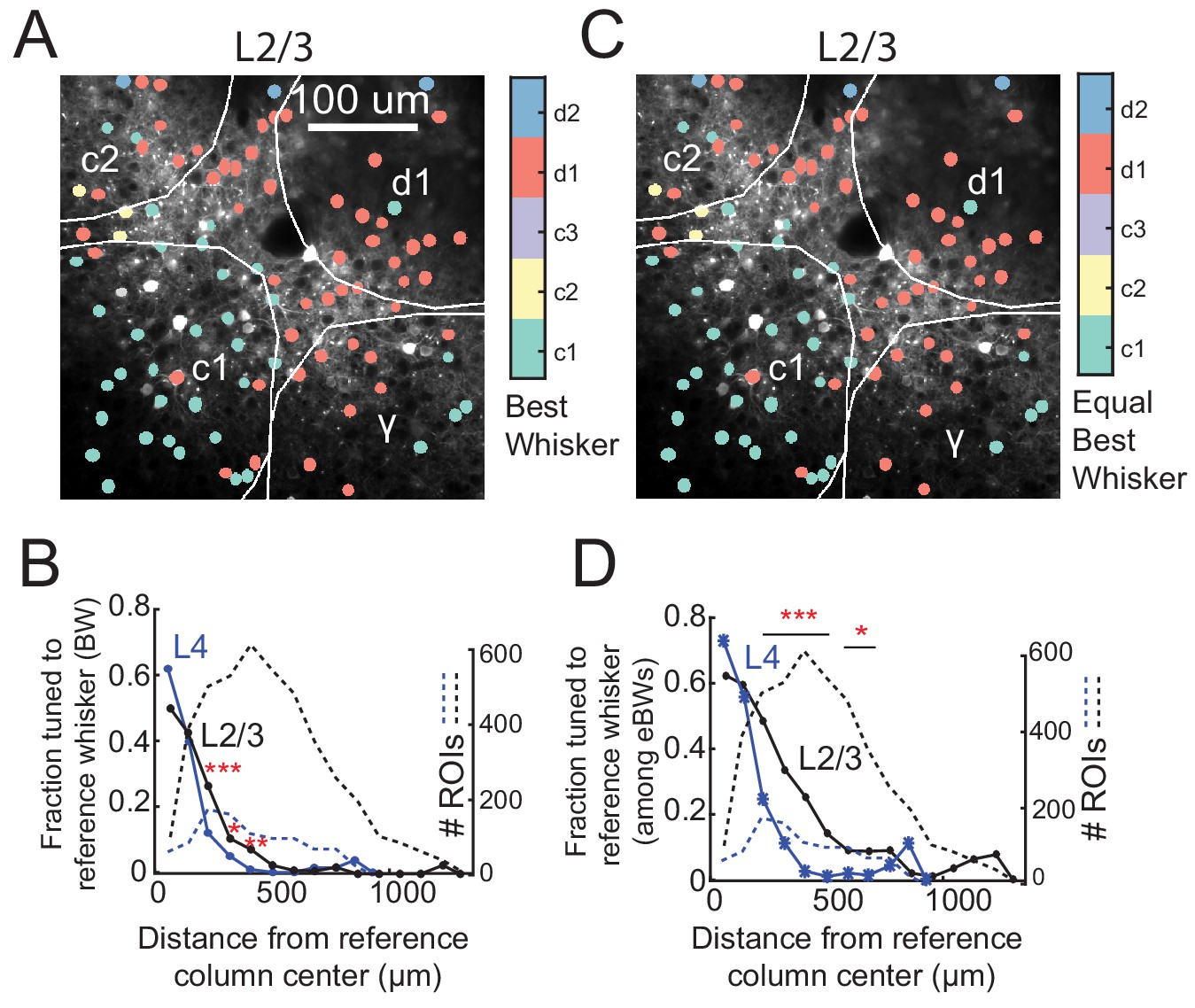
Effect of enrichment on somatotopic tuning precision.
(A) Fraction of L2/3 PYR ROIs tuned to a reference whisker in EN and NH mice. Asterisks show significant differences between EN and NH by Fisher’ Exact Test, computed separately in each spatial bin. *p<0.05, **p<0.01, ***p<0.001. A neuron was considered tuned for the whisker if that whisker was among the equal best whiskers (eBWs). (B) Example L2/3 imaging fields with neurons color-coded by whisker tuning. Left, Normally housed; right, Enriched. White lines denote barrel boundaries. Neurons located over septa and neurons located over barrels that were not tuned to the corresponding columnar whisker are color coded to the whisker which evoked the largest response magnitude. Neurons located over barrels are color coded to the columnar whisker if it evoked the largest response, or evoked a response that was statistically indistinguishable from the largest response. (C–D) As in A and B, for L4 excitatory neurons.
Figure 3—figure supplement 1
Salt-and-pepper tuning organization among L2/3 and L4 excitatory cells in normally housed mice.
(A) Example L2/3 imaging field with ROIs color-coded by the whisker that evoked that largest absolute response. (B) Fraction of responsive excitatory ROIs that were tuned to a reference whisker (defined as evoking the absolute largest response) in spatial bins of distance from that whisker’s anatomical column center. L2/3, black. L4, blue. Dashed lines, number of ROIs in each bin. (C) Same imaging field as (A), with neurons inside each column re-colored to the columnar whisker if it was either the cell’s absolute best whisker, or evoked a response that was statistically indistinguishable from the absolute best whisker. These neurons are ‘equivalently tuned’ to the CW, meaning they are either tuned or co-tuned for the CW. (D) Fraction of L2/3 PYR ROIs equivalently tuned to a reference whisker as a function of distance from the reference whisker column center. Asterisks show significant differences between L4 and L2/3 by Fisher’s Exact Test, computed separately in each spatial bin. *p<0.05, **p<0.01, ***p<0.001.
Figure 4 with 2 supplements
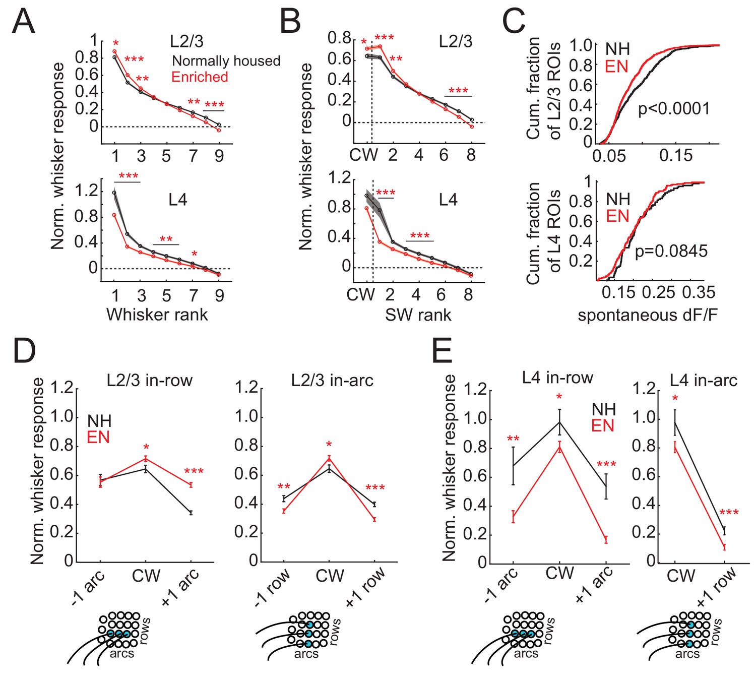
Enrichment sharpens whisker tuning curves.
(A) Mean receptive field for all responsive ROIs, calculated after ranking whiskers from strongest to weakest in each cell and normalizing median responses to spontaneous activity. Asterisks, significant difference between EN and NH, computed separately by permutation test for each whisker rank. *p<0.05, **p<0.01, ***p<0.001. (B), Mean receptive fields separated into CW and ranked SW whiskers. (C) Effect of enrichment on spontaneous activity, defined as median ΔF/F during blank trials. P-values computed by permutation test. (D) Mean responses of L2/3 ROIs to CWs and adjacent whiskers within the same row (left) or the same arc (right). Lower panels: schematics of adjacent whiskers within rows or arcs on the whisker pad. (E) As in D, for L4 ROIs. Only columns containing at least 3 ROIs were included in this analysis. Because most ROIs were located in the C row, no data was available for responses to surround whiskers within the same arc but −1 row relative to the CW. Asterisks, significant difference between EN and NH. *p<0.05, **p<0.01, ***p<0.001.
Figure 4—figure supplement 1
Response magnitude and tuning sharpness analyzed without normalization to spontaneous activity.
Correlation of mean ΔF/F evoked by four weakest whiskers to four strongest whiskers within each L2/3 cell for NH (A) and EN (B). Each dot on scatter plots indicates one neuron. Red lines indicate linear regression fit. Histograms show distribution of absolute evoked response magnitude. ** denotes greater mean response for EN than NH (p=0.0002, permutation test). Note: in EN (B), one point at (0.03, 0.17) is omitted from scatter plot due to scale. Regression slope was different between NH and EN (p=1.2e-9, t-test for difference in slopes).
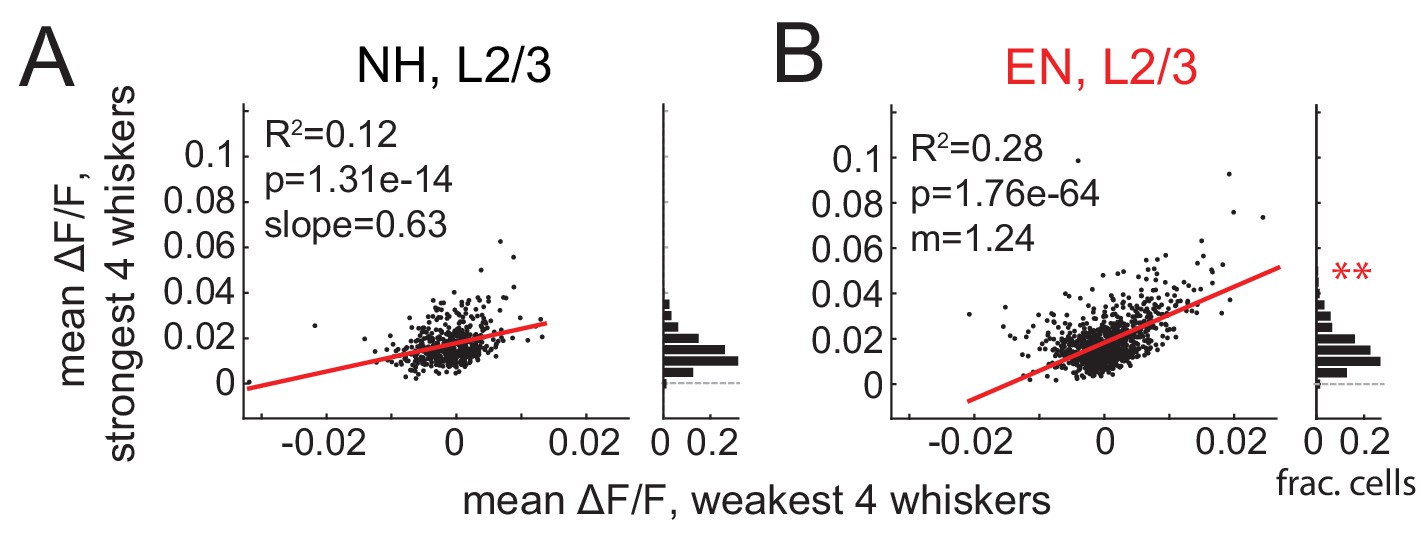
Figure 4—figure supplement 2
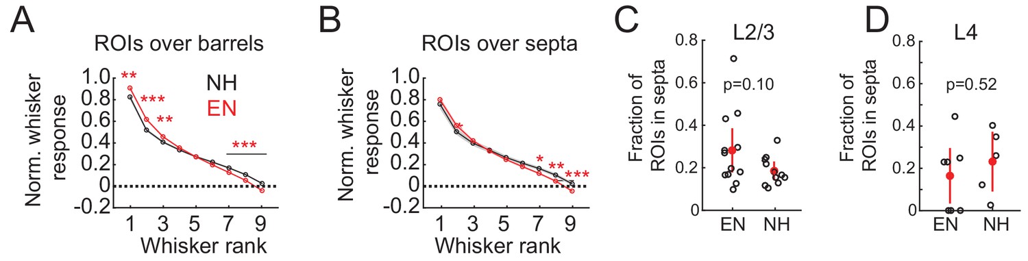
Sharpening of tuning is more prominent for L2/3 neurons overlying L4 barrels than L4 septa.
(A–B) Effect of enrichment on average ranked whisker tuning curves for barrel-related (A) and septal-related (B) ROIs in L2/3. Plots as described in Figure 4A. (C–D) Fraction of whisker-responsive ROIs located over septa in L2/3 (C) or in septa in L4 (D) imaging fields. Each circle represents one imaging field. Red is population mean and SEM. P-values computed from 2-sample t-test.
Figure 5 with 2 supplements
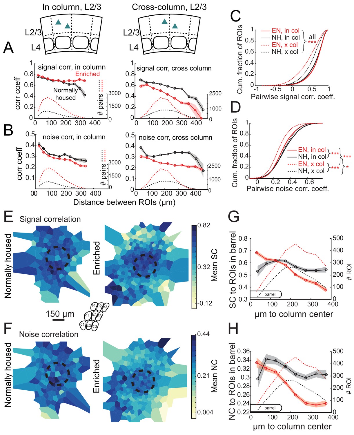
Enrichment alters the spatial structure of signal and noise correlations in L2/3.
(A) Mean signal correlation across responsive L2/3 cell pairs as a function of inter-ROI distance, for cell pairs within a column (left) or across columns (right). Shaded regions denote SEM. Dashed, number of cell pairs in each bin. Insets show schematic of cell locations. (B) Mean noise correlation across all responsive L2/3 pairs, plotted as in (A). (C–D) Cumulative distribution of signal correlation (C) or noise correlation (D) for all within-column (in-col) and across-column (x-col) pairs. Asterisks denote difference between distributions computed by ANOVA with multiple comparisons correction. (E) Spatial map of mean signal correlation for sample ROIs within a position bin to all ROIs located within a reference whisker column. For each sample ROI, the mean signal correlation to all ROIs within the reference column was calculated. Sample ROIs were then clustered into spatial bins, and the mean signal correlation for each bin was plotted. The dashed circle is the reference column (shown as an average barrel diameter around the column center). (F) Spatial map of mean noise correlation to all ROIs within the reference whisker column, shown as in (E). (G) Mean signal correlation from sample ROIs to all cells in a reference column, as a function of sample ROI distance from column center. Shading is SEM. (H) Same as for (G), but for noise correlations. G-H show that enrichment steepens correlation gradients at column edges.
Figure 5—figure supplement 1
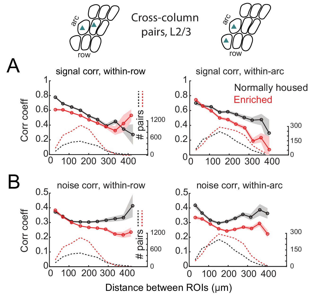
Spatial structure of signal and noise correlations across rows and arcs in L2/3.
(A) Mean signal correlation across responsive L2/3 cell pairs located across columns as a function of inter-ROI distance, for cell pairs across columns within a row (left) or across columns within an arc (right). Shaded regions denote SEM. Dashed, number of cell pairs in each bin. Insets above plots show schematic of cell locations. (B) Mean noise correlation across all responsive L2/3 pairs located across columns within a row (left) or within an arc (right), plotted as in (A).
Figure 5—figure supplement 2
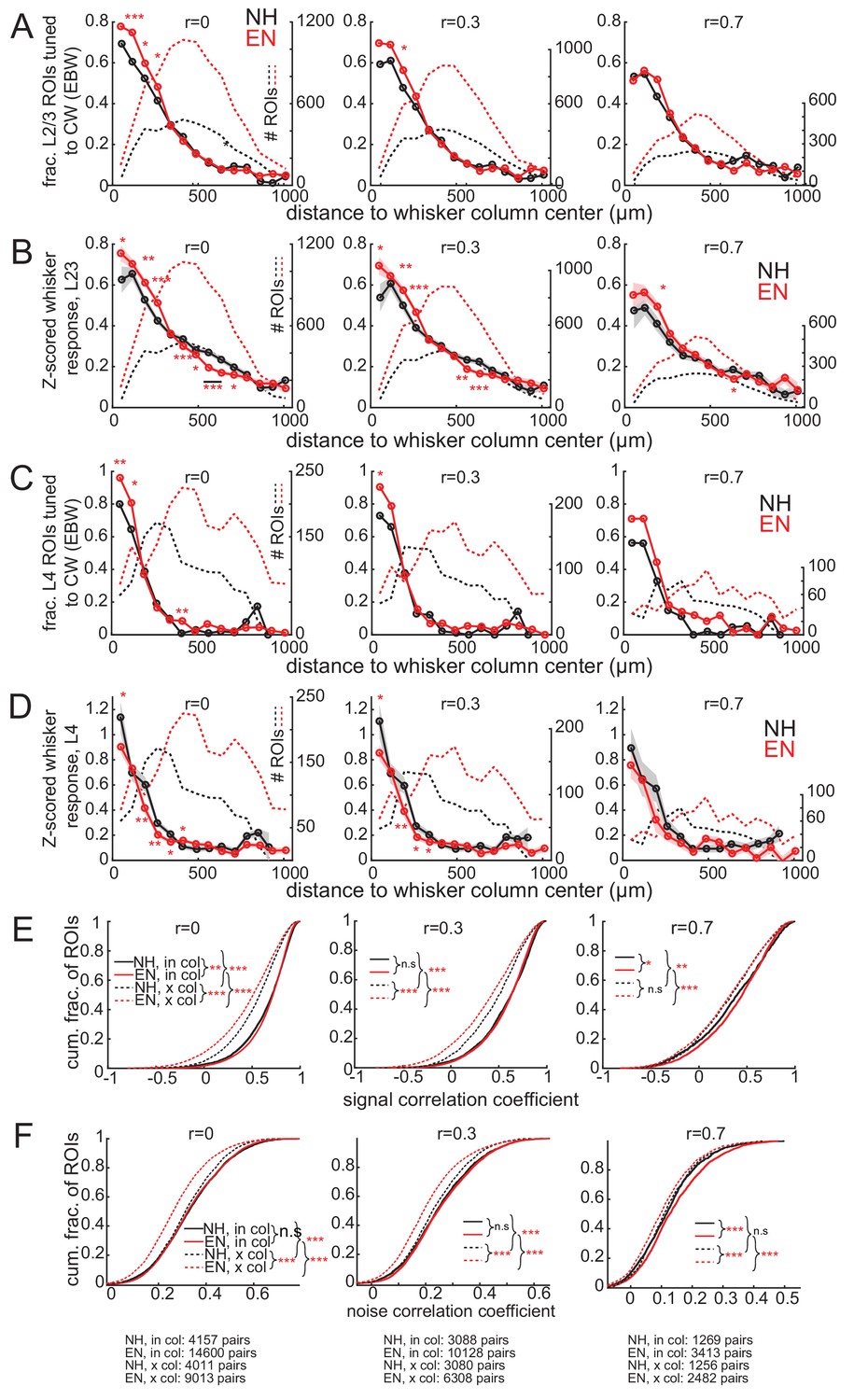
Neuropil subtraction minimally impacts the major effects of the study.
(A–F) The principal effects of EN recalculated under different levels of neuropil subtraction. Neuropil subtraction was performed by calculating the raw fluorescence of each ROI on each frame as . Left column, r = 0 (no neuropil subtraction). Middle column, r = 0.3. Right, r = 0.7. (A) Fraction of L2/3 PYR ROIs tuned to a reference whisker, calculated as in Figure 3A. Asterisks show significant differences between EN and NH by Fisher’ Exact Test, computed separately in each spatial bin. *p<0.05, **p<0.01, ***p<0.001. (B) Mean response evoked by a reference whisker, calculated and plotted as in Figure 2A. (C) Same as in (A), but for L4 excitatory cells. (D) Same as in in (B), for L4 excitatory cells. (E–F) Distribution of signal correlation (E) or noise correlation (F) for all within-column (in-col) and across-column (x-col) L2/3 PYR pairs. Plotted as in Figure 5D and E. Asterisks denote difference between distributions computed by ANOVA with multiple comparisons correction. The bottom row in (F) reports numbers of pairs of significantly whisker-responsive ROIs at each neuropil subtraction weight.
Figure 6

Enrichment increases signal and noise correlations within L4 barrels.
(A) Mean signal correlation across responsive L4 cell pairs as a function of inter-ROI distance, for cell pairs within a column. Conventions as in Figure 6A. Inset, schematic of cell locations. (B) Mean noise correlation across within-column pairs, plotted as in (A). (C–D) Cumulative distribution of signal correlations (C) or noise correlations (D) for within-barrel ROI pairs in L4.
Figure 7
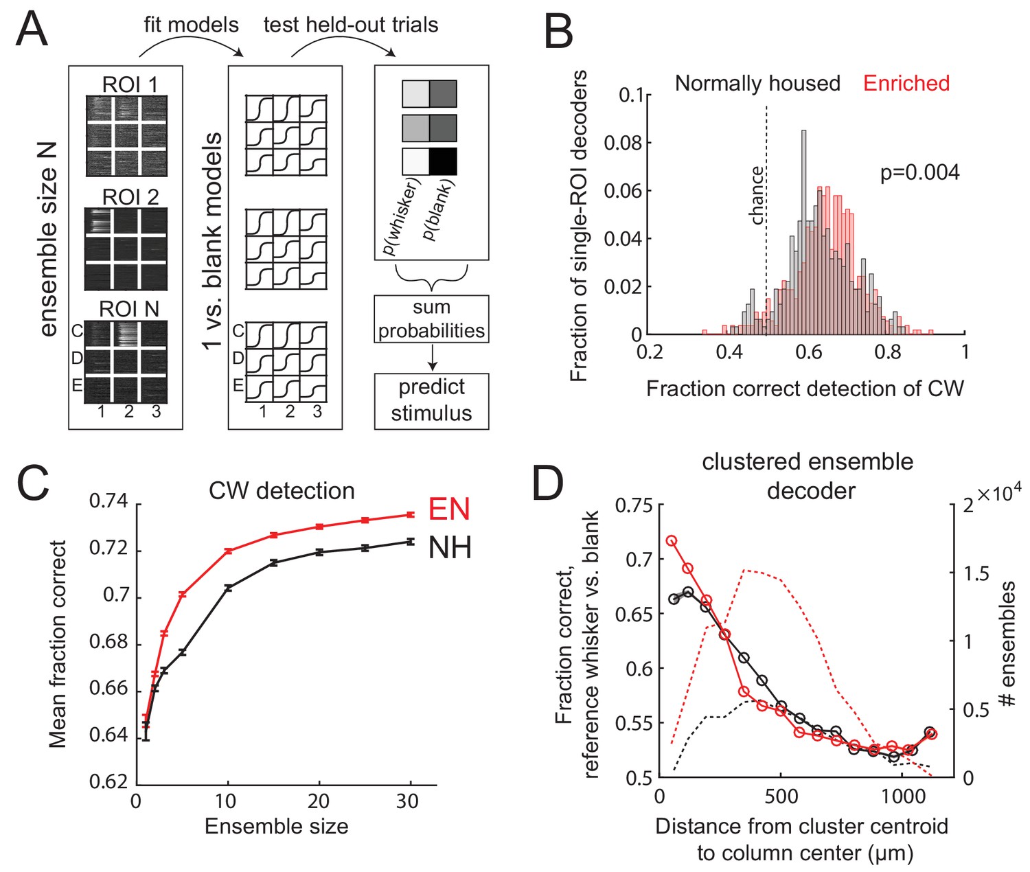
Enrichment improves population coding of CW deflections.
(A) Design of neural decoder for detecting a whisker deflection. (B) Performance of single-ROI decoders on detection of CW deflection vs. blank (no whisker deflection). (C) Detection performance for population decoders of varying size. Each ensemble decoder consisted of randomly positioned, simultaneously imaged ROIs, and was tested on detection of the whisker closest to the centroid of the ensemble. Bars show SEM. (D) Detection of a reference whisker deflection by ensemble decoders located at varying distances from the reference column. These were spatially clustered ensembles of 2–42 simultaneously imaged ROIs (see Materials and methods). Distance bins refer to distance between reference column center and the centroid of each ensemble.
Author response image 1
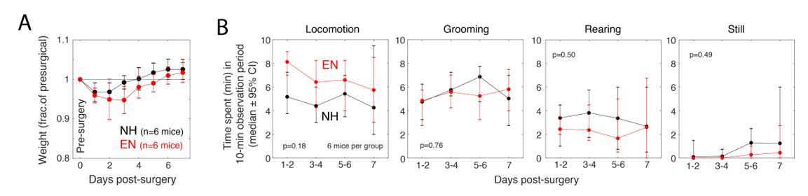
Comparison of surgical recovery between NH and EN mice.
Data are from a new cohort of 6 NH and 6 EN mice, all C57BL/6 wild-types. Surgery for headplate and cranial window implant was on Day 0. A. Daily weight during surgical recovery. Mean recovery to pre-surgical weight was 4 days (NH) or 5.5 days (EN). B. Spontaneous behaviors quantified in a clean open-field environment. Time spent in each behavior was calculated with 30-sec resolution. ‘Still’ indicates 30-sec periods in which neither locomotion, grooming or rearing occurred. Behavior was recorded daily and analyzed in 2-day windows. Circles and bars are bootstrapped medians and 95% confidence intervals. P-values are for permutation test for difference between NH and EN in total area under the curve. There were no significant differences between NH and EN in any behavior (α = 0.05).
Tables
Table 1
Mouse information.
https://doi.org/10.7554/eLife.46321.004| Age at imaging | sex | Days enriched | Days expressing GcaMP6s | N mice | N imaging fields | |
|---|---|---|---|---|---|---|
| Drd3-Cre; NH | P56 ± 11 | 2F, 5M | n/a | 17 ± 2 | 7 | 11 |
| Drd3-Cre; EN | P59 ± 12 | 2F, 5M | 37 ± 13 | 20 ± 5 | 7 | 11 |
| Scnn1-Tg3-Cre; NH | P70 ± 16 | 2F, 3M | n/a | 39 ± 12 | 5 | 6 |
| Scnn1-Tg3-Cre; EN | P58 ± 5 | 5F, 1M | 35 ± 4 | 28 ± 5 | 6 | 8 |
| all Drd3-Cre | P58 ± 11 | 4F, 10M | 37 ± 13 | 18 ± 4 | 14 | 22 |
| all Scnn1-Tg3-Cre | P64 ± 14 | 7F, 4M | 35 ± 4 | 34 ± 11 | 11 | 14 |
Key resources table
| Reagent type (species) or resource | Designation | Source or reference | Identifiers | Additonal information |
|---|---|---|---|---|
| Genetic reagent (M. musculus) | Scnn1a-tg3-Cre line | Jackson Labs | RRID:IMSR_JAX:009613 | |
| Genetic reagent (M. musculus) | Drd3-Cre line | MMRRC | RRID:MMRRC_034610-UCD | |
| Recombinant DNA reagent | AAV1.Syn.Flex.GCaMP6s.WPRE.SV40 | Penn Vector Core | Penn: AV-1-PV2821 | |
| Recombinant DNA reagent | AAV9.CAG.Flex.GCaMP6s.WPRE.SV40 | Penn Vector Core | Penn: AV-9-PV2818 | |
| Software, algorithm | MATLAB (version 2014b) | Mathworks | RRID:SCR_001622 | |
| Software, algorithm | ScanImage | Vidrio Technologies | RRID:SCR_014307 | |
| Software, algorithm | Igor Pro (version 6) | Wave Metrics | RRID:SCR_000325 |
Additional files
-
Transparent reporting form
- https://doi.org/10.7554/eLife.46321.018
Download links
A two-part list of links to download the article, or parts of the article, in various formats.
Downloads (link to download the article as PDF)
Open citations (links to open the citations from this article in various online reference manager services)
Cite this article (links to download the citations from this article in formats compatible with various reference manager tools)
Enrichment drives emergence of functional columns and improves sensory coding in the whisker map in L2/3 of mouse S1
eLife 8:e46321.
https://doi.org/10.7554/eLife.46321


