Figures and data in Mechanisms of chromosome biorientation and bipolar spindle assembly analyzed by computational modeling

Figures
Videos
Tables
Additional files

8 figures, 8 videos, 8 tables and 3 additional files

Figures

Figure 1

Download asset Open asset

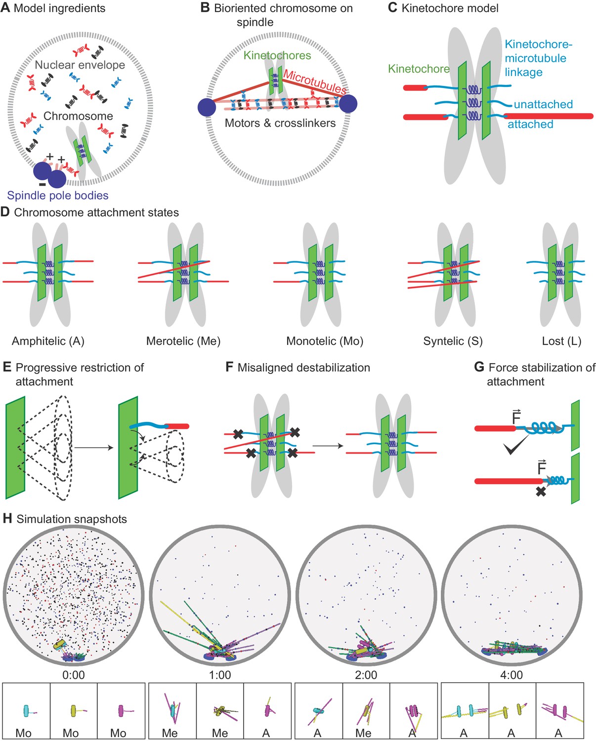
Schematic of computational model and simulation of the reference model.

(A) Schematic of initial condition, showing adjacent spindle-pole bodies (blue) embedded in the nuclear envelope (gray dashed), proximal chromosomes (gray with green plate and blue springs), short microtubules (pink), and motor proteins and crosslinkers (red, blue, and black). (B) Schematic of bipolar spindle and a bioriented chromosome. (C) Schematic of chromosome and kinetochore model showing sister chromatids (gray), one kinetochore on each chromatid (green plates), the pericentric chromatin spring (blue springs), and kinetochore-MT attachment factor (blue line). (D) Schematic of chromosome attachment states, showing amphitelic, merotelic, monotelic, syntelic, and lost chromosomes. (E) Schematic of progressive restriction, showing that the angular range of kinetochore-MT attachment is restricted after attachment. (F) Schematic of misaligned destabilization of attachment, showing that misaligned attachments are destabilized. (G) Schematic of force stabilization of attachment, showing that end-on attachment to depolymerizing MTs has increased lifetime. (H) Image sequence of spindle assembly and chromosome biorientation rendered from a three-dimensional simulation. Initially, spindle-pole bodies (SPBs) are adjacent (blue disks), MTs are short spherocylinders (green and purple when unattached to kinetochores, yellow and magenta when attached), and chromosomes (cyan, yellow, magenta) are near SPBs. Motors and crosslinkers are dispersed spots (red, blue, and black) within the nucleus (gray boundary). Time shown in minutes:seconds. Lower: a zoomed view of each chromosome with attachment state labeled.

Figure 1—source data 1 Configuration files for the simulations used for snapshots in Figure 1H.: https://cdn.elifesciences.org/articles/48787/elife-48787-fig1-data1-v2.gz.zip
Download elife-48787-fig1-data1-v2.gz.zip

Figure 2 with 1 supplement

Download asset Open asset

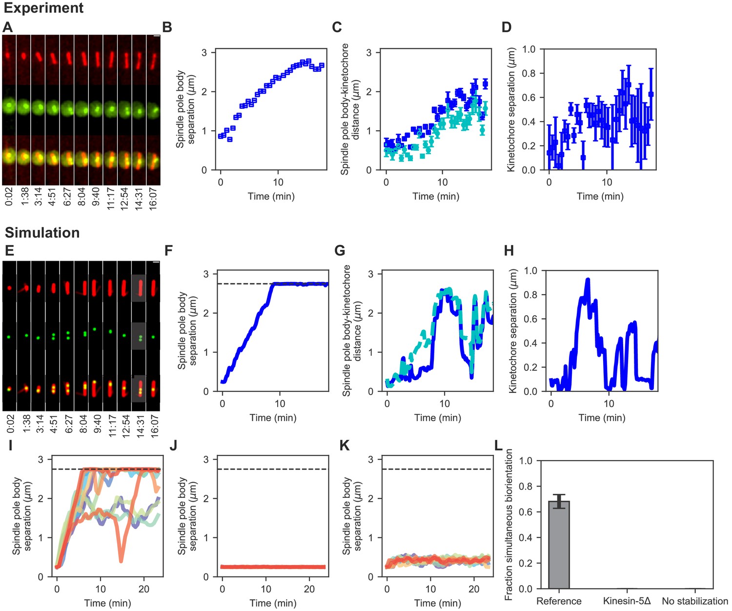
Comparison of spindle assembly and chromosome alignment in cells and simulations.

(**A–D**) Experimental results. (A) Maximum-intensity-projected smoothed images from time-lapse confocal fluorescence microscopy of fission yeast with *mCherry-atb2* labeling MTs (red) and *cen2-GFP* labeling the centromere of chromosome 2 (green). Time shown in minutes:seconds. (B) Spindle length, (C) spindle pole body-kinetochore distance, and (D) interkinetochore distance versus time for the experiment shown in (A). (**E–K**) Simulation results. (E) Simulated fluorescence microscopy images with MTs (red) and a single kinetochore pair (green). (F) Spindle length, (G) spindle pole body-kinetochore distance, and (H) interkinetochore distance versus time from the simulation shown in (E), sampled at a rate comparable to the experimental data in (**A–D**). Note that the rigid nucleus in our model sets an upper limit on spindle length of 2.75 μm, as shown by the dashed line in F. (I) Spindle length versus time for 12 simulations of the reference model. (J) Spindle length versus time for 12 simulations in a model lacking kinesin-5. (K) Spindle length versus time for 12 simulations in a model lacking crosslink-mediated microtubule stabilization. (L) Fraction of simultaneous biorientation for the reference, kinesin-5 delete, and no-stabilization models (N = 12 simulations per data point).

Figure 2—source data 1 Configuration and data files for the simulations used in Figure 2. Configuration files are contained within *config.tar.gz. Data are contained within *data.csv files.: https://cdn.elifesciences.org/articles/48787/elife-48787-fig2-data1-v2.gz.zip
Download elife-48787-fig2-data1-v2.gz.zip

Figure 2—figure supplement 1

Download asset Open asset

Results of simulations with perturbations to motor and crosslinker number, motor force-dependent unbinding, and nuclear envelope rigidity.

(A) Simulated spindles form and biorient chromosomes in the absence of kinesin-14 motors if kinesin-5 and crosslinker number are increased. (B) Simulated spindles have difficulty forming in the absence of crosslinkers, and do not properly biorient chromosomes. (C) Lowering the characteristic distance of force-dependent unbinding of kinesin-14 to that of kinesin-5 (which makes kinesin-14 motors less sensitive to force-induced unbinding) causes longer spindles to form that are capable of biorienting chromosomes. (D) Spindle length as a function of wall force for a model of a soft nuclear envelope for which the SPBs are not fixed on the surface of the sphere. The reference model contains 174 kinesin-5 motors, 230 kinesin-14 motors, and 657 crosslinkers. (N = 12 simulations per data point.).

Figure 2—figure supplement 1—source data 1 Configuration and data files for simulations used in Figure 2—figure supplement 1. Configuration files are contained within the *config.tar.gz files. Data are contained within the MATLAB scripts *panelA-D.m.: https://cdn.elifesciences.org/articles/48787/elife-48787-fig2-figsupp1-data1-v2.gz.zip
Download elife-48787-fig2-figsupp1-data1-v2.gz.zip

Figure 3 with 1 supplement

Download asset Open asset

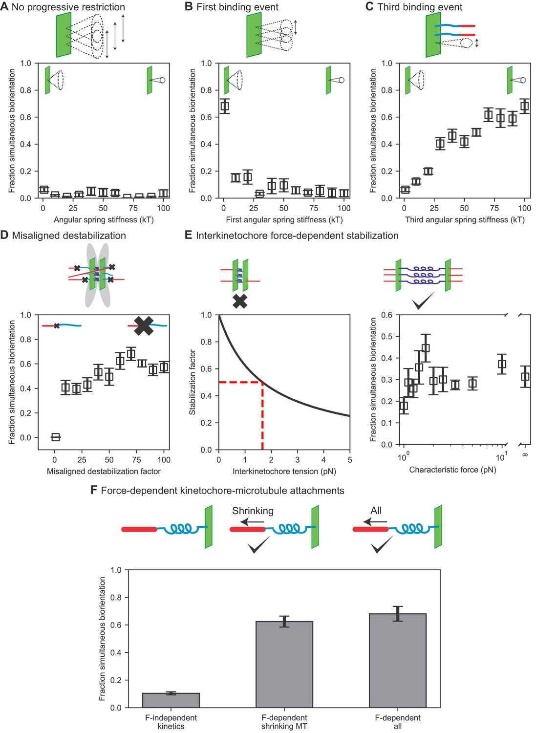
Results of perturbing kinetochore properties required for biorientation.

(A) Fraction simultaneous biorientation versus angular spring stiffness in models lacking progressive restriction of attachment. (B) Fraction simultaneous biorientation versus the first angular spring stiffness in the model with progressive restriction. (C) Fraction simultaneous biorientation versus the third angular spring stiffness in the model with progressive restriction. (D) Fraction simultaneous biorientation versus the misaligned destabilization factor. (E) Effects of force-dependent error correction. Top, schematic of stabilization of kinetochore-MT attachments as a function of interkinetochore force. Left, Stabilization as a function of interkinetochore tension for a characteristic force of 1.67 pN. When the interkinetochore force is the characteristic force, attachment turnover is reduced by a factor of two, as shown by the red dashed lines. Right, fraction simultaneous biorientation versus the characteristic force. (F) Fraction simultaneous biorientation for different types of force-dependent kinetics (N = 12 simulations per data point).

Figure 3—source data 1 Configuration and data files for simulations used in Figure 3. Configuration files are contained within *config.tar.gz. Data are contained within *data.csv files, except for Figure 3E, where the data are contained within the python script Figure 3e_graphcreation.py.: https://cdn.elifesciences.org/articles/48787/elife-48787-fig3-data1-v2.gz.zip
Download elife-48787-fig3-data1-v2.gz.zip

Figure 3—figure supplement 1

Download asset Open asset

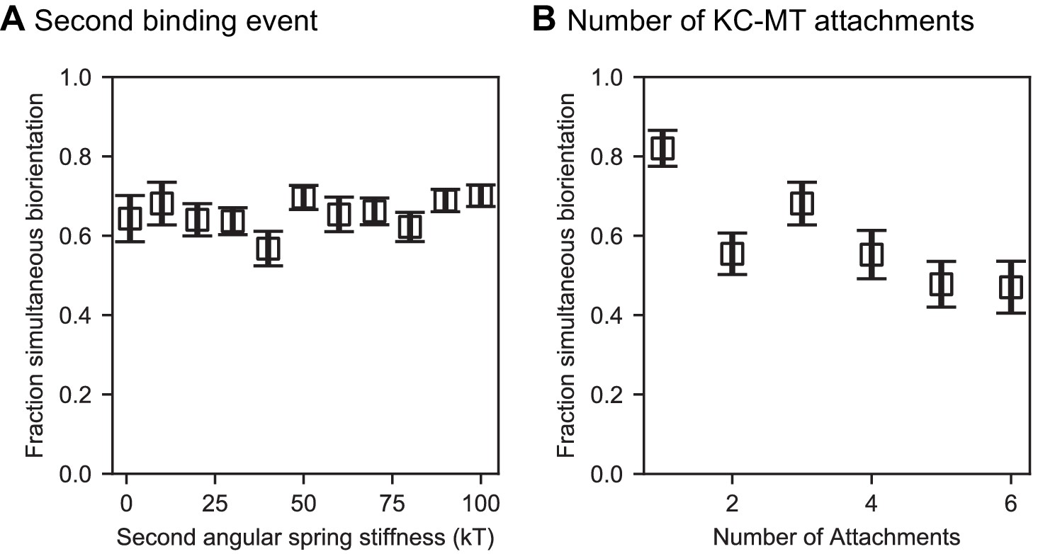
Effects of varying the middle angular stiffness for progressive restriction and the number of kinetochore-microtubule attachments.

(A) Angular spring stiffness for the middle value chosen in progressive restriction did not affect chromosome biorientation fidelity. In these models, the first and third angular spring stiffnesses were fixed at 1 $k_{B} T$ and 100 $k_{B} T$ , respectively. (B) Varying the number of microtubule attachment sites per kinetochore does not significantly alter biorientation in the model. We varied the angular spring stiffnesses are varied with the number of attachments shown as (1: [1 $k_{B} T$ , 1 $k_{B} T$ ], 2: [1 $k_{B} T$ , 10 $k_{B} T$ , 10 $k_{B} T$ ], 3: Reference model, 4–6: [1 $k_{B} T$ , 10 $k_{B} T$ , 100 $k_{B} T$ , 100 $k_{B} T$ , … 100 $k_{B} T$ ]) (N = 12 simulations per data point).

Figure 3—figure supplement 1—source data 1 Configuration and data files for simulations used in Figure 3—figure supplement 1. Configuration files are contained within the *config.tar.gz files. Data are contained within the *data.csv files.: https://cdn.elifesciences.org/articles/48787/elife-48787-fig3-figsupp1-data1-v2.gz.zip
Download elife-48787-fig3-figsupp1-data1-v2.gz.zip

Figure 4

Download asset Open asset

Changes in kinetochore-MT attachment turnover alter spindle length fluctuations.

(**A–C**) Spindle length versus time for 24 simulations of the same model, with (A) short (1/4 the reference value), (B) intermediate (1/2 the reference value), and (C) long (twice the reference value) kinetochore-MT attachment lifetime. (D) Length fluctuation magnitude versus measured kinetochore-MT attachment lifetime and average interkinetochore stretch (color) for bioplar spindles (corresponding to simulation time >10 min.). (E) Length fluctuation magnitude versus measured kinetochore-MT attachment lifetime and average interkinetochore stretch (color) for the reference, restricted, and weak rescue models (N = 24 simulations per data point).

Figure 4—source data 1 Configuration and data files for simulations used in Figure 4. Configuration files are contained within *config.tar.gz files for the noted panels. Figure 4A–C data contained within *data.csv files that pertains to the spindle length versus time measurements. Data for panels Figure 4D,E are contained in their respective files as well, but contain data for the kinetochore-microtubule attachment lifetimes and length fluctuations measurements.: https://cdn.elifesciences.org/articles/48787/elife-48787-fig4-data1-v2.gz.zip
Download elife-48787-fig4-data1-v2.gz.zip

Figure 5

Download asset Open asset

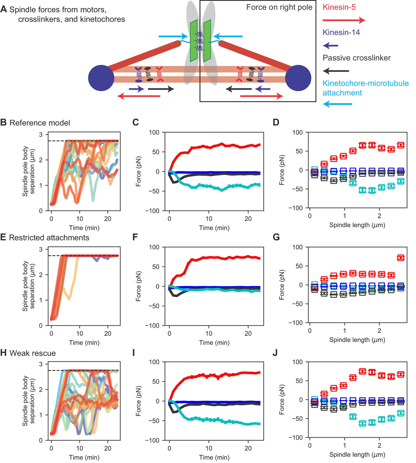
Spindle force generation varies as the spindle assembles and elongates.

(A) Schematic of force generation along the spindle axis, showing kinesin-5 motors exerting outward force (red) and kinesin-14 (dark blue), crosslinkers (black), and kinetochore-MT attachment to stretched chromosomes (light blue) exerting inward force. (**B, E, H**) Spindle length versus time, (**C, F, I**) average spindle axis force versus time, and (**D, G, J**) average spindle axis force versus spindle length for three different models: (**B–D**) the reference model, (**E–G**) the restricted attachment model, and (**H–J**) the weak rescue model (N = 24 simulations per data point).

Figure 5—source data 1 Configuration and data files for simulations used in Figure 5. Configuration files are contained within *config.tar.gz files for the noted panels. Spindle length versus time measurements are found within Figure 5b,e,h_data.csv files. Spindle force measurements are found within Figure 5cd,fg,ij_data.csv files.: https://cdn.elifesciences.org/articles/48787/elife-48787-fig5-data1-v2.gz.zip
Download elife-48787-fig5-data1-v2.gz.zip

Figure 6

Download asset Open asset

Chromosome segregation in the model and comparison to experiments.

(A) Image sequence of simulation of chromosome segregation after anaphase is triggered, rendered from a three-dimensional simulation. Anaphase begins immediately after the first image. Lower, schematic showing kinetochore position along the spindle. Time shown in minutes:seconds. (**B–D**) Simulation results. (B) Simulated fluorescence microscopy images with MTs (red) and a single kinetochore pair (green). Time shown in minutes:seconds. (C) Spindle pole body-kinetochore distance, and (D) interkinetochore distance versus time from the simulation shown in (B), sampled at a rate comparable to the experimental data in (**E–G**). (**E–G**) Experimental results. Maximum-intensity projected smoothed images from time-lapse confocal fluorescence microscopy of fission yeast with *mCherry-atb2* labeling MTs (red) and *cen2-GFP* labeling the centromere of chromosome 2 (green). Time shown in minutes:seconds. (E) Spindle length, (F) spindle pole body-kinetochore distance, and (G) interkinetochore distance versus time from the experiment shown in (E).

Figure 6—source data 1 Configuration and data files for simulations used in Figure 6. Configuration files are contained within *config.tar.gz files for the noted panels. Spindle length data are found within the *data.csv files.: https://cdn.elifesciences.org/articles/48787/elife-48787-fig6-data1-v2.gz.zip
Download elife-48787-fig6-data1-v2.gz.zip

Appendix 1—figure 1

Download asset Open asset

Chromosome model overview.

(A) Chromosomes are modeled as sister chromatids and kinetochores held together by a cohesin/chromatin spring complex. Each kinetochore can attach up to three microtubules. (B) Steric interactions between MTs and kinetochores prevent overlap, while a soft steric repulsion exists between MTs and the centromeric DNA. (C) Kinetochores are kept back-to-back through a cohesin-chromatin spring complex that depends on relative kinetochore position and orientation. (D) The angular range of kinetochore-MT attachment is restricted based on the stiffness of an angular spring. (E) The angular restriction of kinetochore-MT attachment changes based on the number of bound MTs. (F) Attachments are destabilized when the chromosome is not properly bioriented. (G) Attachment lifetime is force-dependent, with attachments to depolymerizing MTs under tension having longer lifetimes, while those to polymerizing MTs have their lifetime decreased under tension. (H) MT dynamics are force-dependent. Polymerizing MTs have increased growth speed and reduced catastrophe, while depolymerizing MTs have increased rescue and decreased shrinking speed.

Appendix 1—figure 2

Download asset Open asset

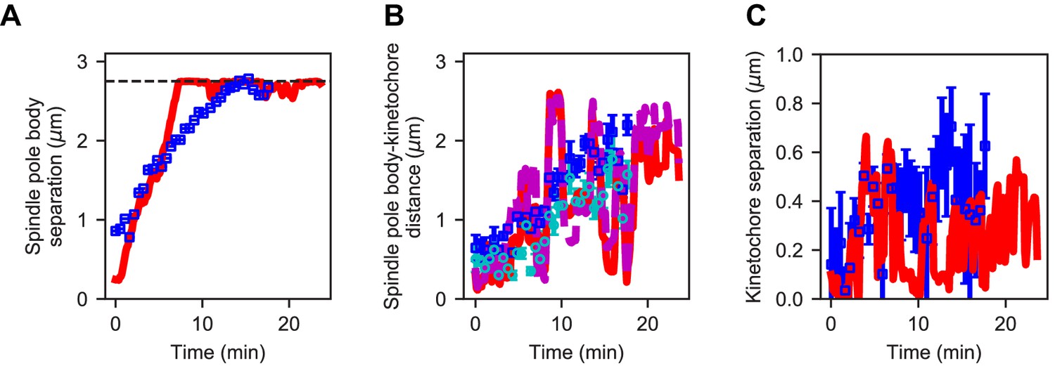
Reference model generates similar dynamics of spindle length and kinetochore position compared to experiment.

(A) Spindle length versus time for experiment (blue) and refined model (red). (B) Spindle pole body-kinetochore distance versus time for a single kinetochore pair (Cen2) in experiment (blue, cyan) and refined model (red, magenta). (C) Kinetochore separation versus time for experiment (blue) and refined model (red). This comparison gives Pearson correlation coefficients for length = 0.891, SPB-KC distance = 0.72, Interkinetochore distance = 0.42.

Videos

Video 1

Download asset

posterframe for video — Simulation of the reference model shows spindle assembly simultaneous with chromosome biorientation.

Initially, short MTs begin to grow at the start of the simulation and interact with nearby kinetochores. A bipolar spindle forms as the chromosomes begin to biorient. Finally, a metaphase spindle is established with bioriented chromosomes that move along the spindle and breathe. The insets are zoomed views of each chromosome, showing attachment turnover and interkinetochore stretch.

Video 2

Download asset

Video 3

Download asset

Video 4

Download asset

Video 5

Download asset

Video 6

Download asset

Video 7

Download asset

Video 8

Download asset

Tables

Table 1

Simulation, SPB, and MT parameters.

Simulation parameter	Symbol	Value	Notes
Time step	$δ t$	8.9 ×10^-6 s	Blackwell et al., 2017a
Nuclear envelope radius	$R$	1.375 μm	Kalinina et al., 2013
Spindle pole bodies
Diameter	$σ_{SPB}$	0.1625 μm	Ding et al., 1993
Bridge size		75 nm	Ding et al., 1993
Tether length	$R_{0}$	50 nm	Flory et al., 2002; Muller et al., 2005
Tether spring constant	$K_{0}$	0.6625 pN nm^-1	Blackwell et al., 2017a
Translational diffusion coefficient	$D_{t}$	4.5 × 10^-4 μm² s^-1	Blackwell et al., 2017a
Rotational diffusion coefficient	$D_{θ, spb}$	0.0170 s^-1	Blackwell et al., 2017a
Linkage time	$τ_{l i n k}$	5 s	Blackwell et al., 2017a
Microtubules
Diameter	$σ_{M T}$	25 nm	Blackwell et al., 2017a
Angular diffusion coefficient	$D_{θ}$	Depends on MT length	Blackwell et al., 2017a; Kalinina et al., 2013
Force-induced catastrophe constant	$α_{c}$	0.5 pN^-1	Blackwell et al., 2017a; Janson et al., 2003; Dogterom and Yurke, 1997
Growth speed	$v_{p, 0}$	4.1 μm min^-1	Blackwell et al., 2017a; Blackwell et al., 2017b
Shrinking speed	$v_{s, 0}$	6.7 μm min^-1	Blackwell et al., 2017a; Blackwell et al., 2017b
Catastrophe frequency	$f_{c, 0}$	3.994 min^-1	Blackwell et al., 2017a; Blackwell et al., 2017b
Rescue frequency	$f_{r, 0}$	0.157 min^-1	Blackwell et al., 2017a; Blackwell et al., 2017b
Growth speed stabilization	$s_{v g}$	1.54	Optimized
Shrinking speed stabilization	$s_{v s}$	0.094	Optimized
Catastrophe frequency stabilization	$s_{f c}$	0.098	Optimized
Rescue frequency stabilization	$s_{f r}$	18	Optimized
Stabilization length	$s_{ℓ}$	16 nm	Optimized
Minimum MT length	$L_{\min}$	75 nm	Optimized

Table 2

Soft nuclear envelope model parameters.

Parameter	Symbol	Value	Notes
Translational mobility	$μ_{SPB}^{t b}$	$(\begin{matrix} 0.05 & 0 & 0 \\ 0 & 0.11 & 0 \\ 0 & 0 & 0.11 \end{matrix}) μ m s^{- 1} p N^{- 1}$	Calculated
Rotational mobility	$μ_{SPB}^{r b}$	$(\begin{matrix} 16.6 & 0 & 0 \\ 0 & 0.166 & 0 \\ 0 & 0 & 0.166 \end{matrix}) μ m^{- 1} s^{- 1} p N^{- 1}$	Calculated
Membrane tube radius	$f_{tube}$	87.7 nm	Derényi et al., 2002; Lim et al., 2007; Lamson et al., 2019
MT asymptotic wall force	$f_{MT, w}$	2.5 pN	Derényi et al., 2002; Lim et al., 2007; Lamson et al., 2019
SPB asymptotic wall force	$f_{SPB, w}$	17 pN	Derényi et al., 2002; Lim et al., 2007; Lamson et al., 2019
Tether spring constant	$K_{0}$	6.625 pN nm^-1	Optimized

Table 3

Motor and crosslinker parameters.

Simulation parameter	Symbol	Value	Notes
Kinesin-5
Number	$N_{K 5}$	174	Optimized (Carpy et al., 2014)
Association constant per site	$K_{a}$	90.9 μM^-1 site^-1	Cochran et al., 2004
One-dimensional effective concentration	$c_{2}$	0.4 nm^-1	Blackwell et al., 2017a
Spring constant	$K$	$0.3 pN {nm}^{- 1}$	Kawaguchi and Ishiwata, 2001
Singly-bound velocity	$v_{0}$	$- 100 nm s^{- 1}$	Roostalu et al., 2011
Polar aligned velocity	$v_{0, P}$	$- 50 nm s^{- 1}$	Gerson-Gurwitz et al., 2011
Anti-polar aligned velocity	$v_{0, A P}$	$8 nm s^{- 1}$	Gerson-Gurwitz et al., 2011
Singly bound off-rate	$k_{1}$	0.11 s^-1	Roostalu et al., 2011
Doubly bound off-rate (single head)	$k_{2}$	0.055 s^-1	Blackwell et al., 2017a
Tether length	$R_{0}$	53 nm	Kashlna et al., 1996
Stall force	$F_{s}$	5 pN	Valentine et al., 2006
Characteristic distance	$x_{c}$	1.5 nm	Optimized (Arpağ et al., 2014
Diffusion constant (solution)	$D_{free}$	4.5 $μ m^{2} s^{- 1}$	Bancaud et al., 2009
Kinesin-14
Number	$N_{K 14}$	230	Optimized (Carpy et al., 2014)
Association constant (motor head)	$K_{a, m}$	22.727 μM^-1 site^-1	Chen et al., 2012
Association constant (passive head)	$K_{a, d}$	22.727 μM^-1 site^-1	Blackwell et al., 2017a
1D effective concentration (motor head)	$c_{2 m}$	0.1 nm^-1	Blackwell et al., 2017a
1D effective concentration (passive head)	$c_{2 d}$	0.1 nm^-1	Blackwell et al., 2017a
Spring constant	$K$	$0.3 pN {nm}^{- 1}$	Kawaguchi and Ishiwata, 2001
Singly bound velocity (motor head)	$v_{0 m}$	$- 50 nm s^{- 1}$	Blackwell et al., 2017a
Diffusion constant (bound, diffusing head)	$D_{d}$	0.1 μm² s^-1	Blackwell et al., 2017a
Singly bound off-rate (motor head)	$k_{1 m}$	0.11 s^-1	Blackwell et al., 2017a
Singly bound off-rate (passive head)	$k_{1 d}$	0.1 s^-1	Blackwell et al., 2017a
Doubly bound off-rate (motor head)	$k_{2 m}$	0.055 s^-1	Blackwell et al., 2017a
Doubly bound off-rate (passive head)	$k_{2 d}$	0.05 s^-1	Blackwell et al., 2017a
Tether length	$R_{0}$	53 nm	Blackwell et al., 2017a
Stall force	$F_{s}$	5.0 pN	Blackwell et al., 2017a
Characteristic distance	$x_{c}$	4.8 nm	Optimized (Arpağ et al., 2014)
Adjusted characteristic distance	$x_{c}^{^{'}}$	1.5 nm	Figure 2—figure supplement 1C
Crosslinker
Number	$N_{X L}$	657	Optimized (Carpy et al., 2014)
Association constant	$K_{a}$	90.9 μM^-1 site^-1	Cochran et al., 2004
One-dimensional effective concentration	$c_{2}$	0.4 nm^-1	Lansky et al., 2015
Spring constant	$K$	0.207 pN nm^-1	Lansky et al., 2015
Diffusion constant (solution)	$D_{free}$	4.5 $μ m^{2} s^{- 1}$	Bancaud et al., 2009
Singly bound diffusion constant	$D_{sb}$	$0.1 μ m^{2} s^{- 1}$	Lansky et al., 2015
Doubly bound diffusion constant	$D_{db}$	$6.7 \times 10^{- 3} μ m^{2} s^{- 1}$	Lansky et al., 2015
Singly bound off-rate	$k_{1}$	0.1 s^-1	Kapitein et al., 2008
Doubly bound off-rate	$k_{2}$	0.05 s^-1	Lansky et al., 2015
Parallel-to-antiparallel bindng ratio	$P_{aff}$	0.33	Kapitein et al., 2008; Rincon et al., 2017; Lamson et al., 2019
Characteristic distance	$x_{c}$	2.1 nm	Optimized (Arpağ et al., 2014)
Tether length	$R_{0}$	53 nm	Lansky et al., 2015; Lamson et al., 2019

Table 4

Chromosome and kinetochore parameters.

Simulation parameter	Symbol	Value	Notes
Kinetochore kinematics
Diameter	$σ_{K C}$	200 nm	Blackwell et al., 2017a; Kalinina et al., 2013
Length	$L_{K C, 0}$	150 nm	Ding et al., 1993
Width	$L_{K C, 1}$	50 nm	Ding et al., 1993
Thickness	$d_{KC}$	0 nm	Chosen
Diffusion coefficient	$D_{K C}$	5.9 × 10^-4µm² s^-1	Gergely et al., 2016; Blackwell et al., 2017a; Kalinina et al., 2013
Translational drag	$γ_{K C, t}$	3.51 pN µm^-1 s	Computed
Rotational drag	$γ_{K C, r}$	0.165 pN µm s	Computed
Catastrophe enhancement	$s_{KC - cen, fc}$	0.5 pN^-1	Matches NE factor
MT tip length	$l_{cen, tip}$	25 nm	Chosen
Interkinetochore spring
Tether length	$R_{C, 0}$	100 nm	Stephens et al., 2013; Gergely et al., 2016; Gay et al., 2012
Linear spring constant	$κ_{C}$	39 pN µm^-1	Optimized
Rotational spring constant	$κ_{C, u}$	1850 pN nm rad^-1	Optimized
Alignment spring constant	$κ_{C, v}$	1850 pN nm rad^-1	Optimized
Pericentric chromatin
Pericentric chromatin length	$r_{centromere}$	200 nm	Chosen
Pericentric chromatin diameter	$d_{centromere}$	75 nm	Chosen
Kinetochore-centromere offset	$r_{KC - cen}$	37.5 nm	Chosen
Chromatin-MT repulsion amplitude	$A_{CMT}$	1 pN nm	Optimized

Table 5

Attachment factor parameters.

Parameter	Symbol	Value	Notes
Number	$N_{A F}$	3	Ding et al., 1993
Attachment-site separation on kinetochore	$r_{A F, e x}$	40 nm	Ding et al., 1993
Linear spring constant	$κ_{A F, m}$	0.088 pN nm^-1	Optimized
Angular spring constant, 0 to 1	$κ_{A F, r, 0}$	4.1 pN nm	Optimized
Angular spring constant, 1 to 2	$κ_{A F, r, 1}$	41 pN nm	Optimized
Angular spring constant, 2 to 3	$κ_{A F, r, 2}$	410 pN nm	Optimized
Angular spring constant, 3 to 3	$κ_{A F, r, 3}$	410 pN nm	Optimized
Tether length	$r_{A F, 0}$	54 nm	Ciferri et al., 2007
kMC steps	$N_{k m c}$	10	Chosen
MT tip length	$l_{A F, t i p}$	25 nm	Chosen
MT tip crowding	$b_{A F, t i p}$	True	Ding et al., 1993
Tip concentration	$c_{A F, t i p}$	40 nm^-1	Optimized
Side concentration	$c_{A F, s i d e}$	0.4 nm^-1	Optimized
Tip rate assembling	$k_{A F, t i p, a}$	0.0001 s^-1	Optimized
Tip rate disassembling	$k_{A F, t i p, d}$	0.03 s^-1	Optimized
Side rate	$k_{A F, s i d e}$	0.03 s^-1	Optimized
Tip characteristic distance assembling	$x_{c, t, a}$	1 nm	Optimized
Tip characteristic distance disassembling	$x_{c, t, d}$	−3.9 nm	Optimized
Side characteristic distance	$x_{c, s}$	−0.37 nm	Optimized
Angular characteristic factor	$χ_{c}$	0.013	Optimized
Speed	$v_{A F}$	50 nm s^-1	Optimized
Stall force	$f_{A F, s t a l l}$	5 pN	Kinesin-5 (Blackwell et al., 2017a; Akera et al., 2015)
Tip diffusion	$D_{t i p}$	0.0012 μm² s^-1	Optimized
Side diffusion	$D_{s i d e}$	0.018 μm² s^-1	Optimized
Tip tracking	$f_{A F, t r a c k}$	0.25	Optimized
Tip-enhanced catastrophe	$s_{f c, d a m 1}$	4	Optimized
Misaligned destabilization	$s_{k, A B K}$	70	Optimized
Polymerization force factor	$F_{A F, v g}$	8.4 pN	Akiyoshi et al., 2010; Gergely et al., 2016
Depolymerization force factor	$F_{A F, v s}$	−3.0 pN	Akiyoshi et al., 2010; Gergely et al., 2016
Catastrophe force factor	$F_{A F, f c}$	−2.3 pN	Akiyoshi et al., 2010; Gergely et al., 2016
Rescue force factor	$F_{A F, f r}$	6.4 pN	Akiyoshi et al., 2010; Gergely et al., 2016
Maximum polymerization speed	$v_{A F, M T, m a x}$	30 μm min^-1	Gergely et al., 2016

Table 6

Force-dependent error correction model parameters.

Parameter	Symbol	Value	Notes
Inter-kinetochore stabilization force	$F_{E C, 0}$	1.67 pN	Optimized
Rotational spring constant	$κ_{C, u}$	925 pN nm rad^-1	Optimized
Alignment spring constant	$κ_{C, v}$	925 pN nm rad^-1	Optimized
Angular characteristic factor	$χ_{c}$	0.08	Optimized
Side concentration	$c_{A F, s i d e}$	0.32 nm^-1	Optimized
Kinesin-5 number	$N_{K 5}$	200	Optimized

Table 7

Anaphase parameters.

Anaphase	Symbol	Value	Notes
Integrated simultaneous biorientation time	$τ_{S A C}$	4.45 min	Chosen
Anaphase attachment rate	$k_{A F, a n a p h a s e}$	0.00007 s^-1	Chosen
Anaphase MT depoly speed	$v_{a n a p h a s e, s, 0}$	2.2 µm min^-1	Chosen

Appendix 1—table 1

Strain used in this study.

Name	Genotype	Notes
MB 998	cen2::kanr-ura4⁺-lacOp, his7⁺::lacI-GFP, z:adh15:mCherry-atb2:natMX6, leu1-32, h-	This study

Additional files

Source code 1 Code for simulation and analysis framework for confined SPB simulations. Requires C++ compiler, and GSL, GLEW, python2, python3, libyaml, FFTW, GLFW, xQuartz, freeGLUT, libpng, ffmpeg, pkg-config, and png++ libraries. Python libraries should include matplotlib, numpy, opencv-python, panda3d, pandas, PyYAML, and scipy for analysis framework. Used for all simulations except Figure 2—figure supplement 1, panel D: Soft nuclear envelope. Untar and unzip SourceCodeFile1.tar.gz, then use the accompanying Makefile and MakefileIncmk to compile on your system.: https://cdn.elifesciences.org/articles/48787/elife-48787-code1-v2.tar.gz
Download elife-48787-code1-v2.tar.gz
Source code 2 Code for simulation and analysis framework for free SPB simulations. Requires C++ compiler, and armadillo, GSL, GLEW, python2, python3, libyaml, FFTW, GLFW, xQuartz, freeGLUT, libpng, ffmpeg, pkg-config, and png++ libraries. Python libraries should include matplotlib, numpy, opencv-python, panda3d, pandas, PyYAML, and scipy for analysis framework. Used only for Figure 2—figure supplement 1, panel D: Soft nuclear envelope. Untar and unzip SourceCodeFile2.tar.gz, then use the accompanying Makefile and MakefileIncmk to compile on your system.: https://cdn.elifesciences.org/articles/48787/elife-48787-code2-v2.tar.gz
Download elife-48787-code2-v2.tar.gz
Transparent reporting form: https://cdn.elifesciences.org/articles/48787/elife-48787-transrepform-v2.docx
Download elife-48787-transrepform-v2.docx

Download links

A two-part list of links to download the article, or parts of the article, in various formats.

Downloads (link to download the article as PDF)

Open citations (links to open the citations from this article in various online reference manager services)

Mendeley

Cite this article (links to download the citations from this article in formats compatible with various reference manager tools)

Christopher Edelmaier
Adam R Lamson
Zachary R Gergely
Saad Ansari
Robert Blackwell
J Richard McIntosh
Matthew A Glaser
Meredith D Betterton

(2020)

Mechanisms of chromosome biorientation and bipolar spindle assembly analyzed by computational modeling

eLife 9:e48787.

https://doi.org/10.7554/eLife.48787

Share this article

Cite this article

Schematic of computational model and simulation of the reference model.

Figure 1—source data 1

Comparison of spindle assembly and chromosome alignment in cells and simulations.

Figure 2—source data 1

Results of simulations with perturbations to motor and crosslinker number, motor force-dependent unbinding, and nuclear envelope rigidity.

Figure 2—figure supplement 1—source data 1

Results of perturbing kinetochore properties required for biorientation.

Figure 3—source data 1

Effects of varying the middle angular stiffness for progressive restriction and the number of kinetochore-microtubule attachments.

Figure 3—figure supplement 1—source data 1

Changes in kinetochore-MT attachment turnover alter spindle length fluctuations.

Figure 4—source data 1

Spindle force generation varies as the spindle assembles and elongates.

Figure 5—source data 1

Chromosome segregation in the model and comparison to experiments.

Figure 6—source data 1

Chromosome model overview.

Reference model generates similar dynamics of spindle length and kinetochore position compared to experiment.

Simulation of the reference model shows spindle assembly simultaneous with chromosome biorientation.

Top: Simulation of reference model (left) and simulated fluorescence microscopy images (right), with red MTs and green kinetochore (scale bar 1 μm).

Simulation of a model with a soft nuclear envelope and an asymptotic wall force on the SPBs of 17 pN.

Simulations of models with perturbation to kinetochore properties important for biorientation.

Simulation of a model with interkinetochore force-dependent attachments.

Simulations of models with varying kinetochore-MT attachment lifetime.

Simulations of reference, restricted, and weak rescue models.

Simulations of anaphase chromosome segregation.

Simulation, SPB, and MT parameters.

Soft nuclear envelope model parameters.

Motor and crosslinker parameters.

Chromosome and kinetochore parameters.

Attachment factor parameters.

Force-dependent error correction model parameters.

Anaphase parameters.

Strain used in this study.

Source code 1

Source code 2

Transparent reporting form

Downloads (link to download the article as PDF)

Open citations (links to open the citations from this article in various online reference manager services)

Cite this article (links to download the citations from this article in formats compatible with various reference manager tools)