The axonal actin-spectrin lattice acts as a tension buffering shock absorber
- Raman Research Institute, India
- Indian Institute of Science Education and Research, India
- Laboratory of Complex Materials Systems, Paris Diderot University, France
Figures
Figure 1
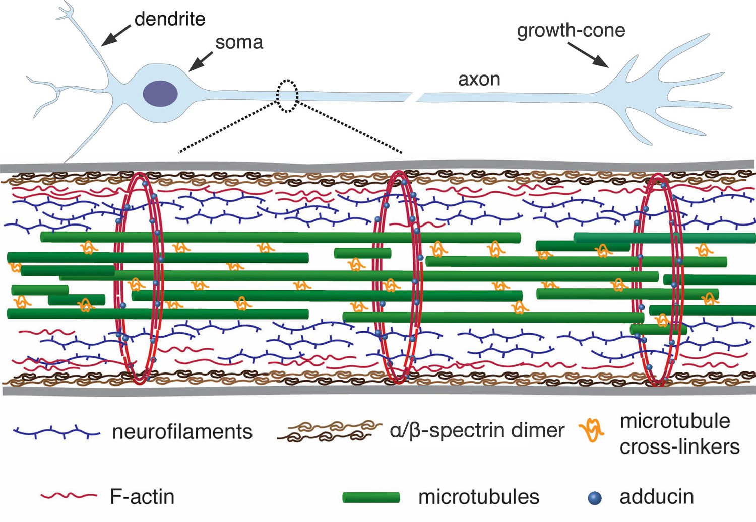
A simplified schematic of the axonal cytoskeleton.
Typically, the axonal core has a bundle of microtubules which are cross-linked by a variety of microtubule-associated proteins which includes tau (in some cases, a more loose organisation of microtubules interdispersed with neurofilaments is seen) (Hirokawa, 1982). This core is surrounded by neurofilaments. The outermost scaffold has an array of periodically spaced rings composed of F-actin filaments. The actin rings are interconnected by -spectrin tetramers, which are aligned along the axonal axis (only tetramers in a cross-section are shown for clarity). Other cortical F-actin structures also exist. A myriad of proteins, including motor proteins (not shown), interconnect the various filaments, and also the membrane (grey lines) to the inner skeleton. The chick DRG axons we use are about 1 µm thick and the rings in them are about 200 nm apart (corresponds to the length of a single tetramer as shown in Refs [Xu et al., 2013; D'Este et al., 2015]).
Figure 2 with 6 supplements
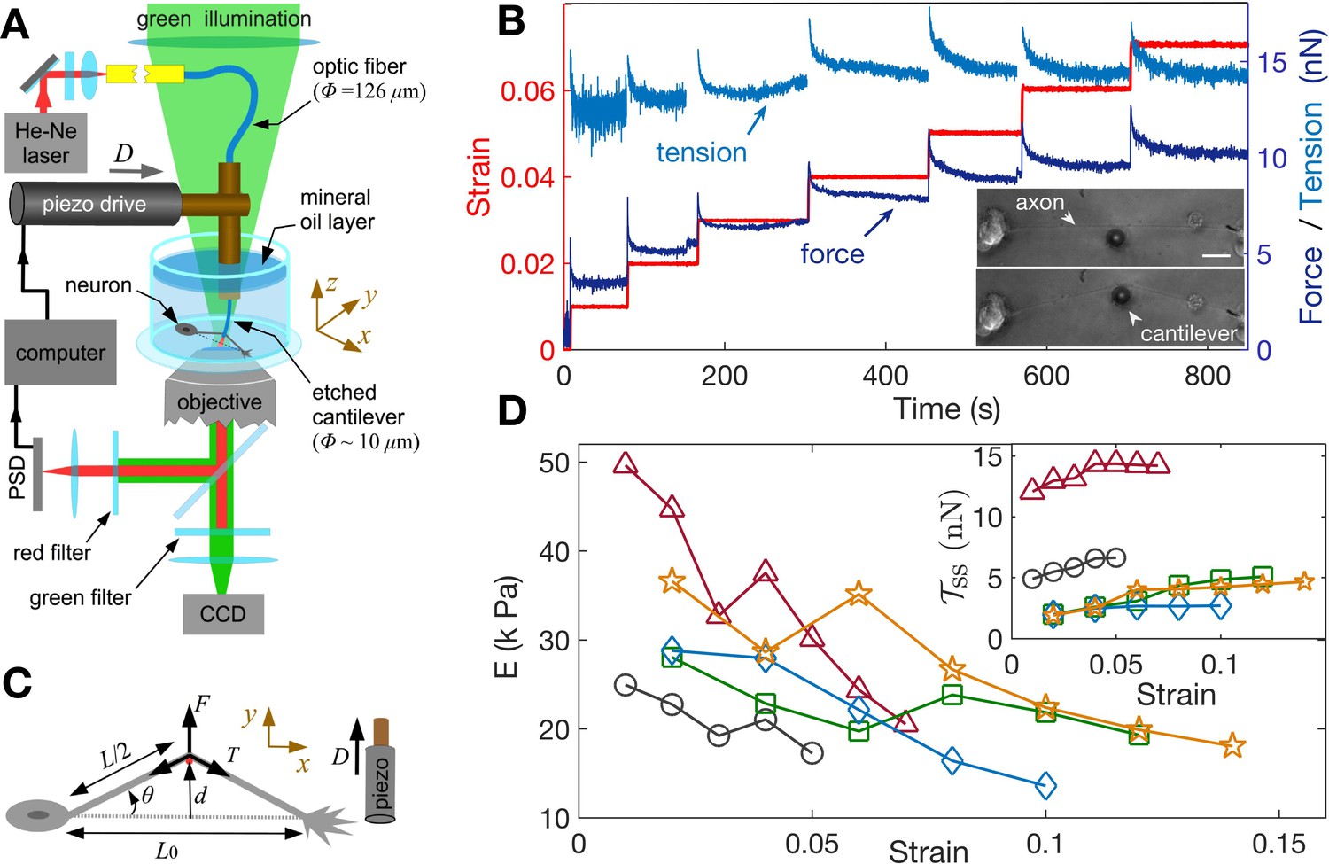
Feedback-controlled axon stretch apparatus reveals strain-softening behavior.
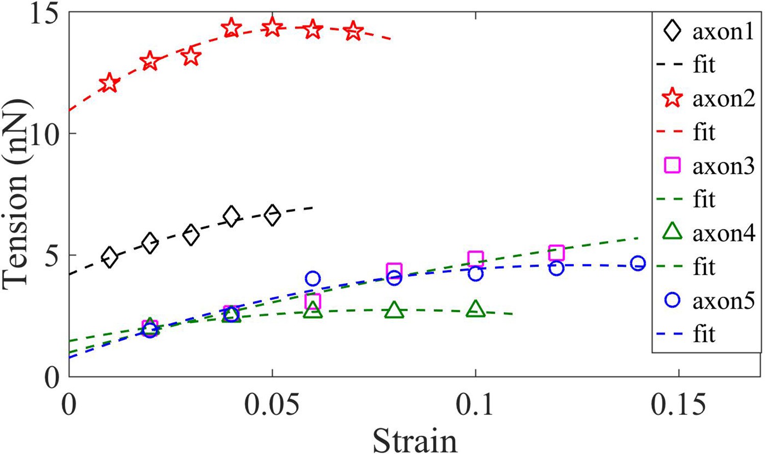
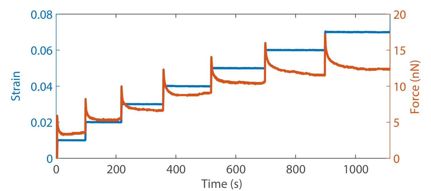
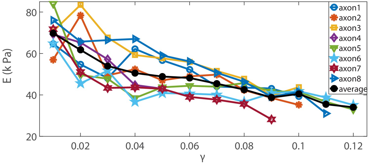
(A) The schematic of the home-developed force apparatus that uses an etched optical fiber as a cantilever to stretch axons and to sense force. Laser light exiting the cantilever tip is imaged on to a Position Sensitive Detector (PSD), which in turn is read by a computer. The computer controls a piezo drive via a feedback algorithm to apply strain steps and then to maintain the strain constant after each step. (B) Typical force response (dark blue) of a 2-DIV axon to increasing strain explored using successive strain steps (red). The calculated tension in the axons (sky blue) is also shown. The inset shows the images of the axon before and after stretch (scale bar: 20 µm). The light exiting the etched optical fiber cantilever can be seen as a bright spot (reduced in intensity for clarity), and this is imaged on to the PSD to detect cantilever deflection. (C) Illustration of the parameters used in the calculations. The strain is calculated as , and force on the cantilever as , where is the cantilever force constant. The axonal tension is , where . (D) Young’s moduli calculated for different 2-DIV axons using the steady state tension after each step show a strain-softening behavior (the different symbols are for different axons). Only a few representative plots are shown for clarity, and more examples are shown in Figure 2—figure supplement 4. The inset shows the tension vs. strain plots for different axons. Tension tends to saturate with increasing strain (tension homeostasis), which leads to the observed softening.
Figure 2—figure supplement 1
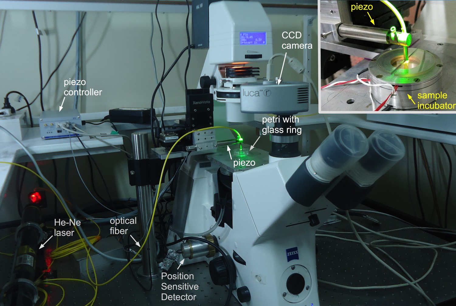
Photograph of the force device.
Photograph of the home developed optical fiber based force apparatus used to investigate the mechanical properties of axons. The piezo drive and the Position Sensitive Detectors are interfaced to a computer to operate the setup in a strain control mode where a feedback loop maintains a prescribed strain value. More details are given in the main text. The inset shows the sample incubator. The etched glass cantilever is not visible in the image but is schematically shown in Figure 2A of the main text and the tip can be seen in the microscope images in Figure 2B.
Figure 2—figure supplement 2
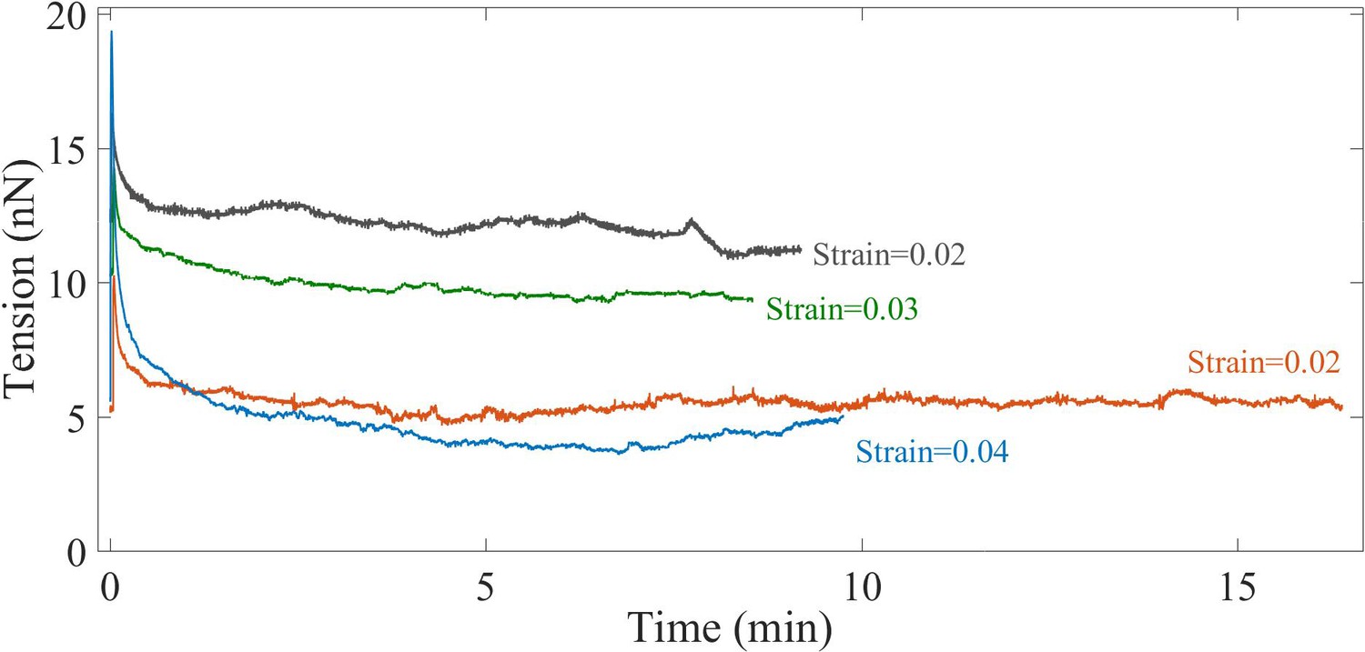
Long time behavior of stretched axons.
Long time axonal response after the application of a single strain step shows that the force relaxes to a steady state value. This shows that axons behave as viscoelastic solid tubes at these timescales.
Figure 2—figure supplement 3
Determination of rest tension .
Axons are under pre-stress (rest tension) even before the application of any strain. This rest tension can be obtained by extrapolating the tension vs strain plot to zero strain. This is done by fitting the data to an equation of the form , which is a simplified form of the tension expression derived from the model presented in the main text.
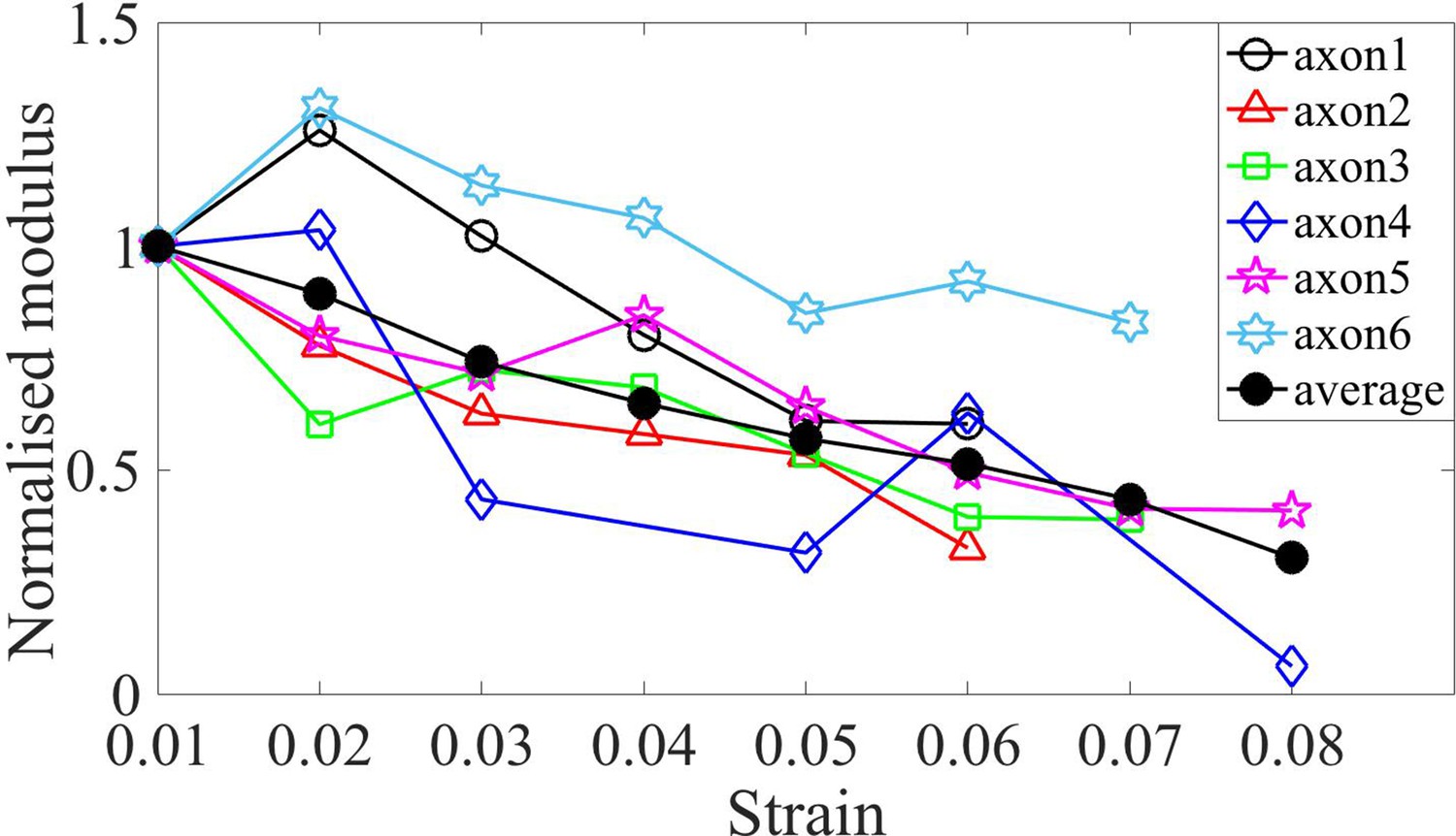
Figure 2—figure supplement 4
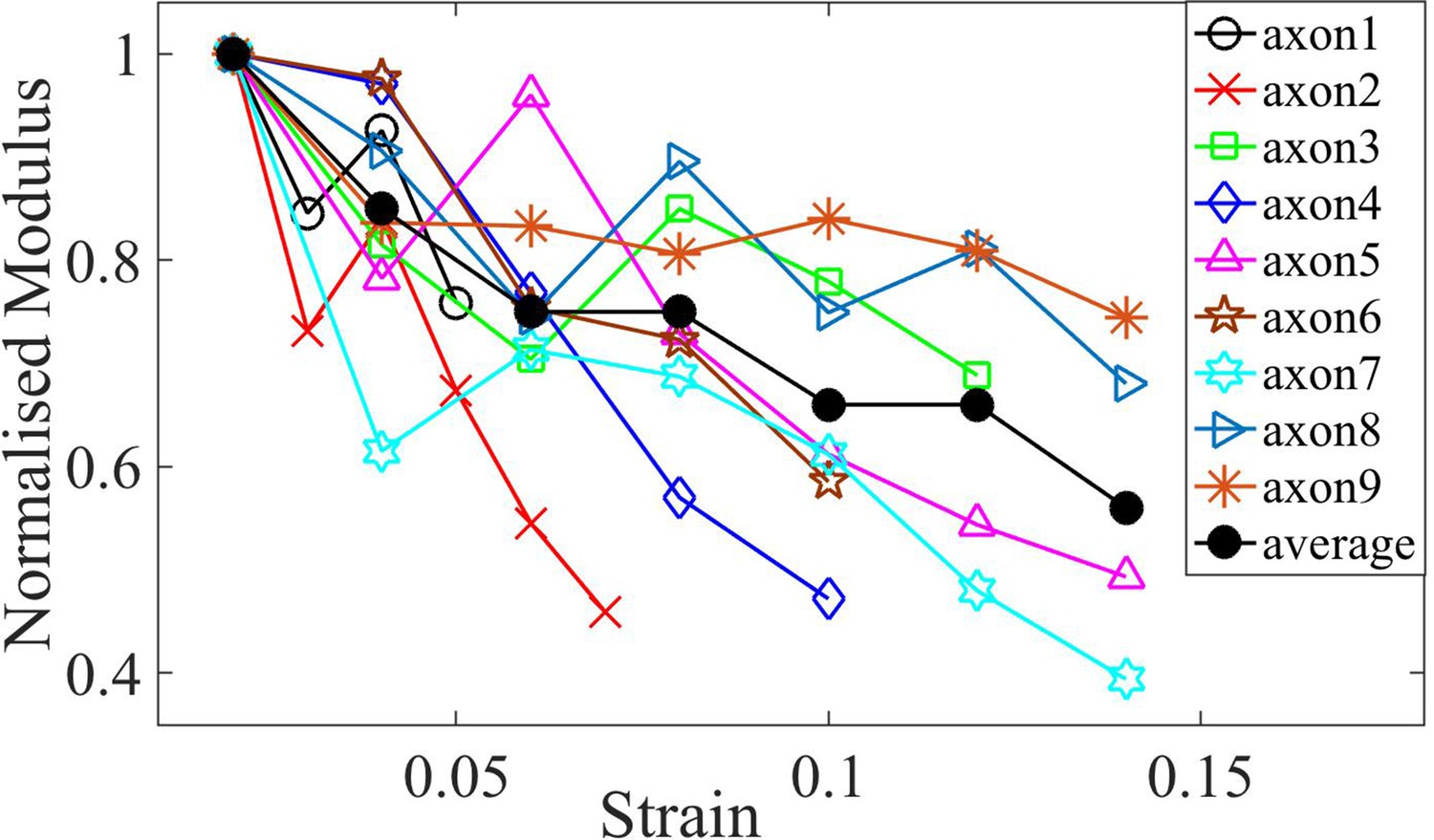
Normalized moduli for control axons.
Elastic moduli for different axons of age 2-DIV normalized by the first strain value which is at 0.02. The plots show softening of modulus with increasing strain. The average is also shown.
Figure 2—video 1
Video showing an axon being stretched using the sequential step-strain protocol.
After each step the strain is held constant via a feedback loop.
Figure 2—video 2
Video showing an axon being released from the cantilever from a pre-stretched state.
Note that the axon recovers its initial length within seconds suggesting that no plastic deformation has occurred.
Figure 3 with 7 supplements
Pharmacological perturbations of the cytoskeleton reveal a key role for F-actin in the axonal stretch response.
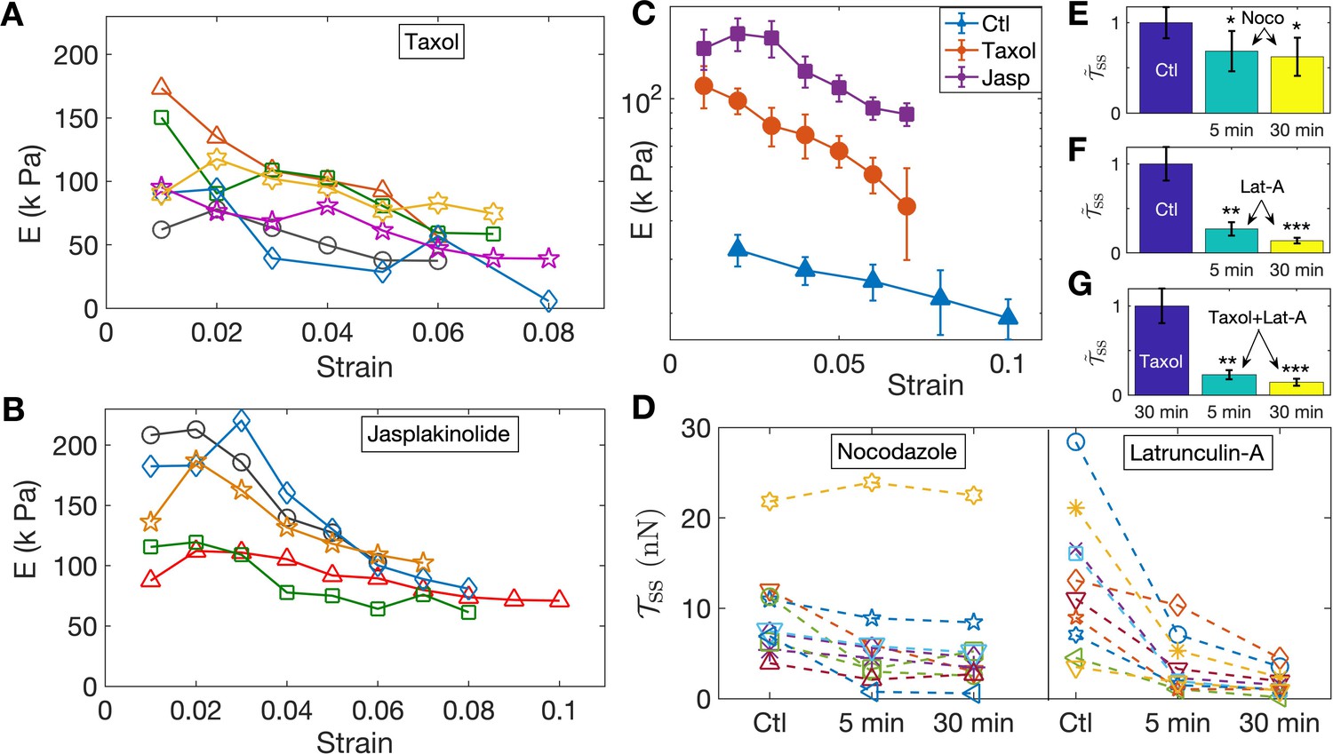
(A,B) Stabilizing microtubules or F-actin by treating 2-DIV axons with either 10 µM Taxol or 5 µM Jasplakinolide leads to significant increases in axonal stiffness, but the strain-softening response persists (more data in Figure 3—figure supplement 6, Figure 3—figure supplement 7; the different symbols are for different axons). (C) Log-linear plots of the averaged elastic moduli as a function of strain for different treatments as well as control (for data shown in A,B and Figure 2D). It can be seen that stabilization of F-actin causes a larger increase in moduli compared to stabilizing microtubules (error bars are standard error (SE)). (D) Change in steady state tension obtained after treating 2-DIV neurons with either the microtubule disrupting drug Nocodazole (10 µM) or the F-actin disrupting drug Latrunculin-A (1 µM) (n = 10 each). These treatments leave the axons very fragile and they detach easily when pulled. Hence a cyclic step-strain protocol with was employed as detailed in the text. As cannot be determined from single steps, we compare the net tension for the same axon before (Ctl) and after 5 min and 30 min of treatment. The data show a significant decrease in axonal tension after F-actin disruption and a relatively smaller decrease after disrupting microtubules. (E, F) Bar plots of steady state tension normalized by that of control showing the significance of the two treatments shown in D. Tension was measured for the same axons 5 min and 30 min after exposing to the drug (error bars are SE). (G) Bar plots of steady state tension normalized by that for Taxol pre-treatment for axons initially treated with Taxol for 30 min, and for the same axons subsequently treated with Lat-A for 5 min and 30 min (n = 7).
Figure 3—figure supplement 1
Force response of Blebbistatin treated cells.
A typical force vs. strain plot for an axon treated with Blebbistatin (myosin-II inhibitor) (30 µM) for 30 mins at 37 °C prior to force measurements. The force vs. strain plot shows qualitatively similar behavior as control axons shown in main text. The elastic moduli for various axons shown below which exhibit strain softening similar to control axons.
Figure 3—figure supplement 2
Elastic moduli of Blebbistatin-treated cells.
Elastic moduli for different axons treated with Blebbistatin, the modulus shows clear strain softening with increasing strain. The average is also shown.
Figure 3—figure supplement 3
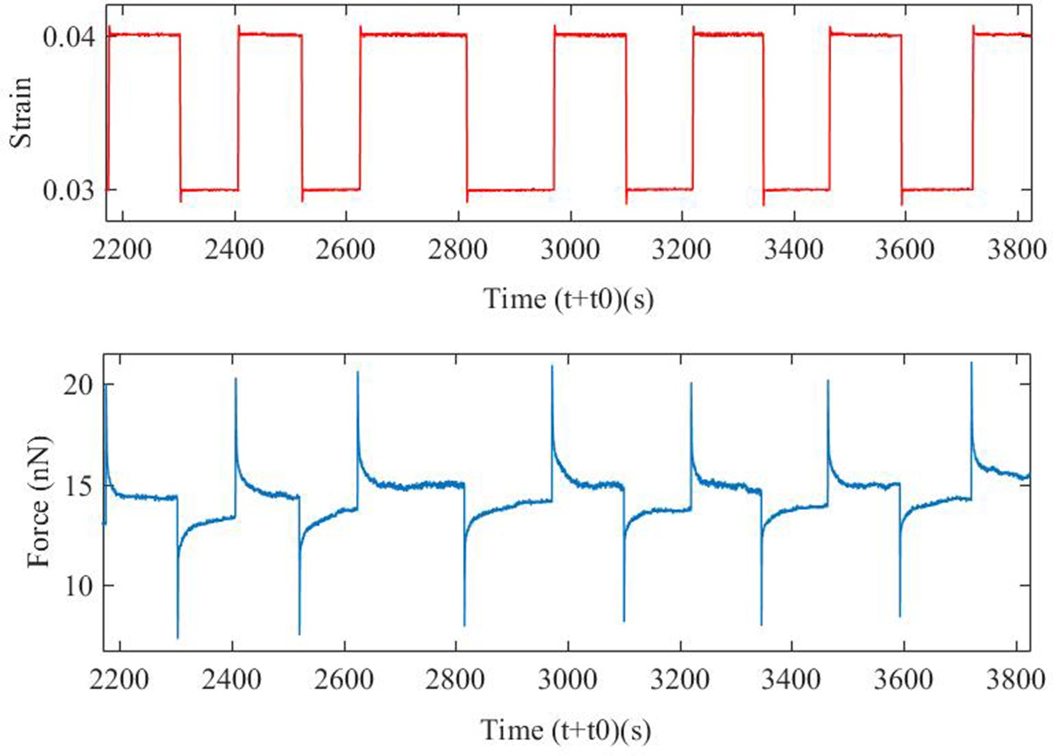
Cyclic strain protocol.
An example of an axon that was pulled to a strain of 3% and then cyclic strain has been applied over an extended period to show that there is no damage with number of cycles. The data also show that the force evolution for up and down steps are similar except for sign. This protocol is then used to study the effect of specific cytoskeleton disrupting agents–Latrunculin-A for F-actin, Nocodazole for microtubules and anti--II spectrin morpholino for spectrin.
Figure 3—figure supplement 4
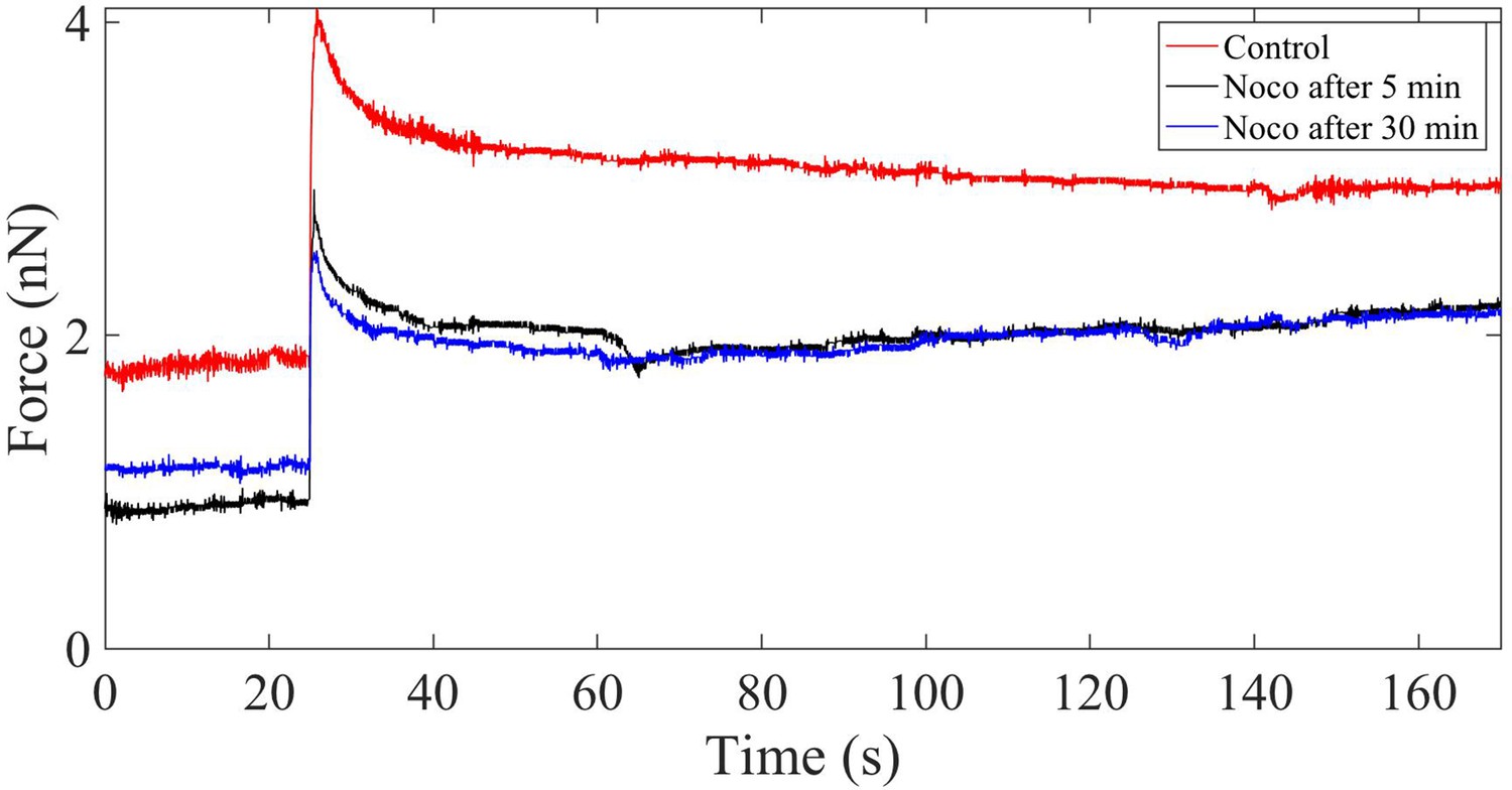
Force relaxation of Nocodazole-treated cells.
Plot showing the force relaxation before and after application of 10 µM Nocodazole (Noco) for 5 min and 30 min. There is no appreciable change in the relaxation time (at 2% strain) after microtubule disruption.
Figure 3—figure supplement 5
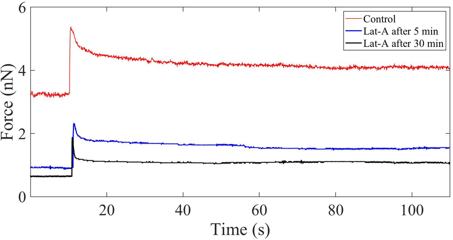
Force relaxation of Latrunculin-A-treated cells.
Plot showing the force relaxation before and after application of 1 µM Latrunculin-A (Lat-A) for 5 min and 30 min. Unlike in the case of microtubule disruption, F-actin depolymerization causes a significant reduction in the modulus (at 2% strain) and the relaxation time.
Figure 3—figure supplement 6
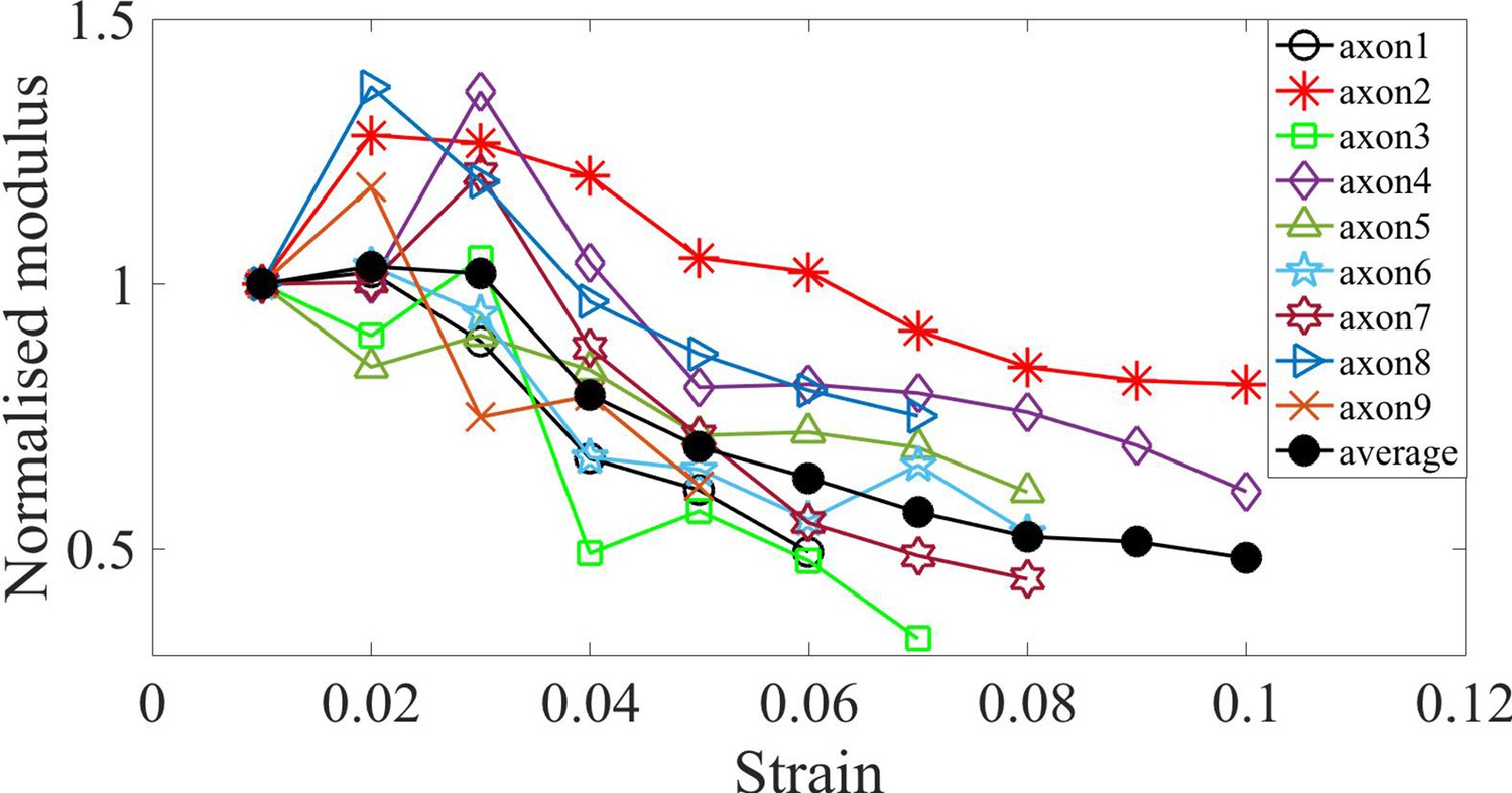
Normalized moduli for Taxol treated cells.
Elastic moduli for different axons treated with Taxol, normalised by the first strain value which is at 0.01, which indicates softening in modulus with increasing strain. The average is also shown.
Figure 3—figure supplement 7
Normalized moduli for Jasplakinolide treated cells.
Elastic moduli for different axons treated with Jasplakinolide, normalized by the first strain value which is at 0.01, which indicates softening in modulus with increasing strain. The average is also shown.
Figure 4 with 7 supplements
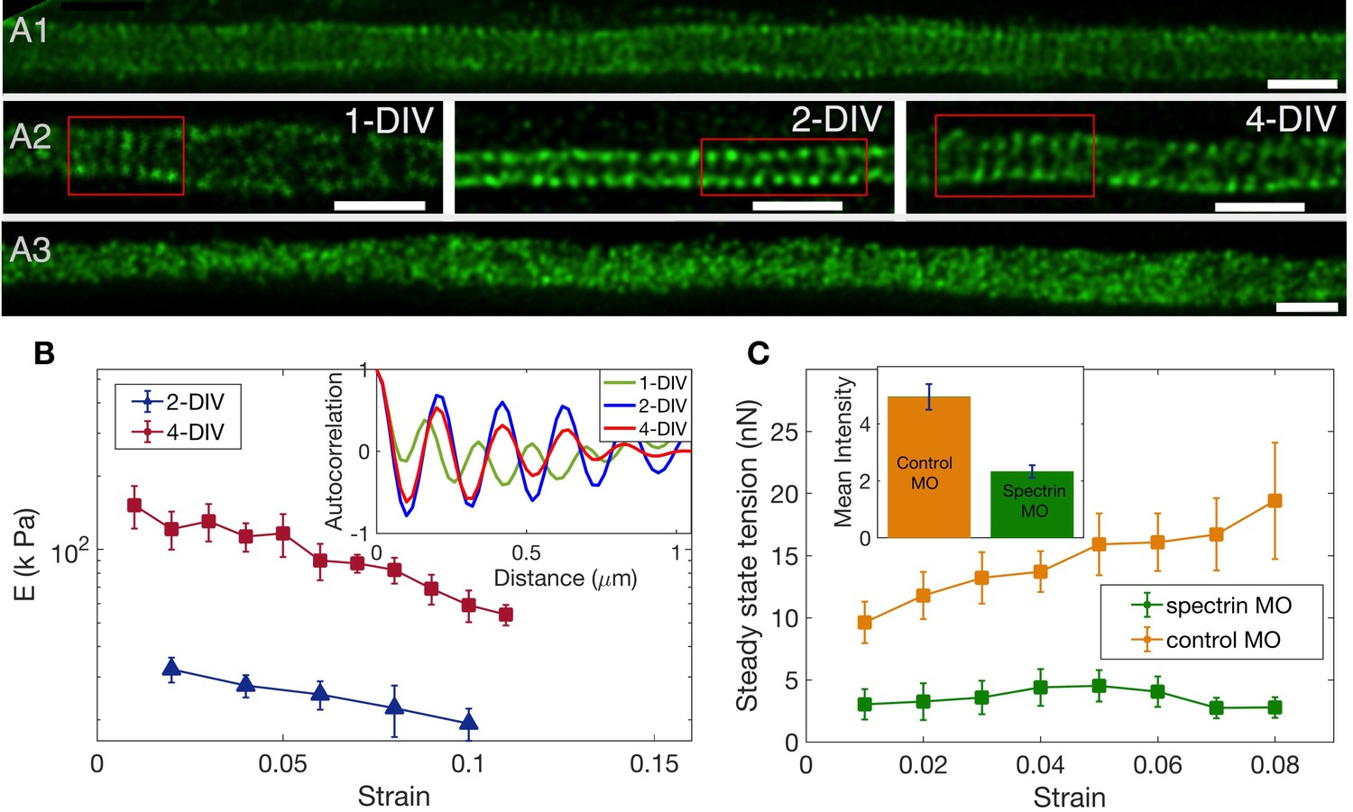
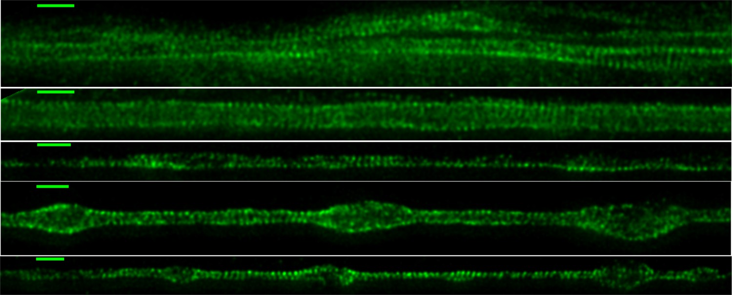
The role of spectrin in axonal mechanics.
(A1) STED nanoscopy image of a 2-DIV axon immunolabelled with -II spectrin antibody (vehicle control). This axon shows rings all along the imaged segment (Figure 4—figure supplement 2 for more examples). (A2) STED images of -II spectrin in control axons of different DIVs. Observation of a large number of axons shows that the spectrin periodicity becomes more prevalent with the age of the axon (see Appendix 1—table 1). (A3) STED image of a 2-DIV axon treated with 1µM Lat-A for 30 min shows disordered -II spectrin intensity distribution (see Figure 4—figure supplement 4 for quantification). All scale bars are 1 µm. (B) Log-linear plots of averaged Young’s modulus vs strain for axons at 2-DIV (n = 5) and 4-DIV (n = 7) show a marked increase in moduli with age (error bars are SE). This increase in moduli correlated with the prevalence of the actin-spectrin lattice as a function of DIV which is quantified in Appendix 1—table 1. The inset shows sample intensity-intensity autocorrelation functions for different DIV axons. The periodicity corresponds to the / spectrin tetramer length which is about 190 nm. (C) Plots of the averaged steady state tension as a function of strain for 2-DIV neurons treated with a non-specific, control morpholino (n = 10) and for those treated with an anti--II spectrin morpholino (n = 10). The non-averaged data for control morpholino are shown in Figure 4—figure supplement 7 for comparison with inset of Figure 2D. The averaged data shows that there is a substantial reduction in the tension measured after knock-down. The inset shows the extent of the knock-down obtained using antibody labelling of spectrin for control (n = 90) and knock-down neurons (n = 91); all error bars indicate the standard error (p < 0.05) (see Materials and methods for details).
Figure 4—figure supplement 1
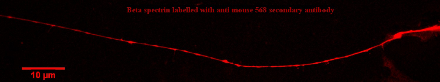
Spectrin distribution in axons (Confocal image).
Confocal image showing spectrin distribution in an axon labelled using a primary antibody anti -II spectrin and a secondary antibody anti-mouse IgG conjugated to Alexa Fluor 568. Spectrin is seen distributed all along all axons of all ages in confocal images. The fine structure has been quantified using Super Resolution as detailed below.
Figure 4—figure supplement 2
Spectrin distribution in axons (STED images).
Super-resolution images of 2-DIV DMSO vehicle control axons labelled using primary antibody anti -II spectrin and secondary antibody anti-mouse IgG conjugated to Alexa Fluor 488. The rings are seen extensively (Scale bar = 1 μm). Some of the disordered patches may be due to fixation process (the presence of beading or bulges which are not seen before fixation suggest this).
Figure 4—figure supplement 3
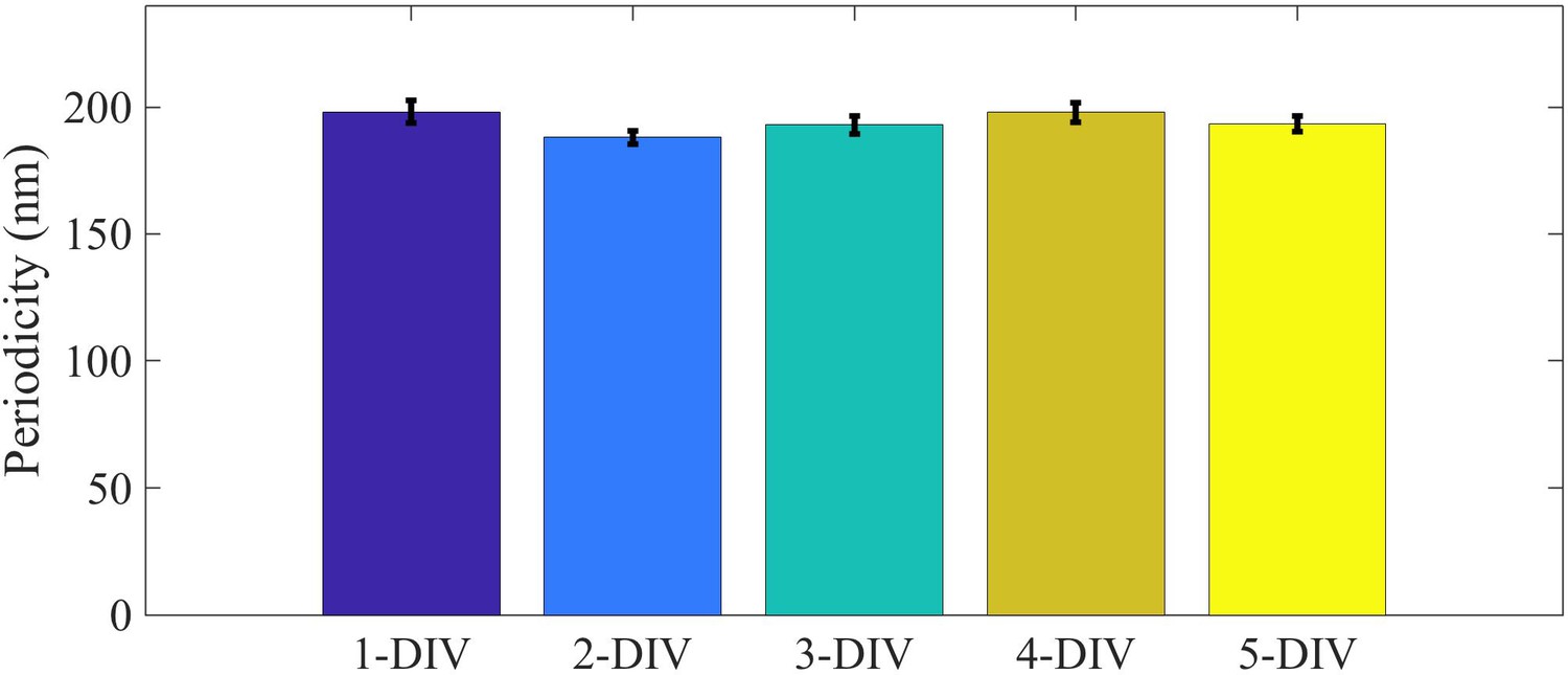
Periodicity of spectrin lattice at various DIV.
Periodicity of spectrin lattice in axons of different age measured using STED microscopy. Number of axons used in each case was n(1-DIV)=23, n(2-DIV)=23, n(3-DIV)=24, n(4-DIV)=20, n(5-DIV)=24 This analysis was done using LAS AF version 3.3.0.10134 from Lieca Micro-systems by drawing a line along the axon and the average distance between adjacent peaks were measured for each axon.
Figure 4—figure supplement 4
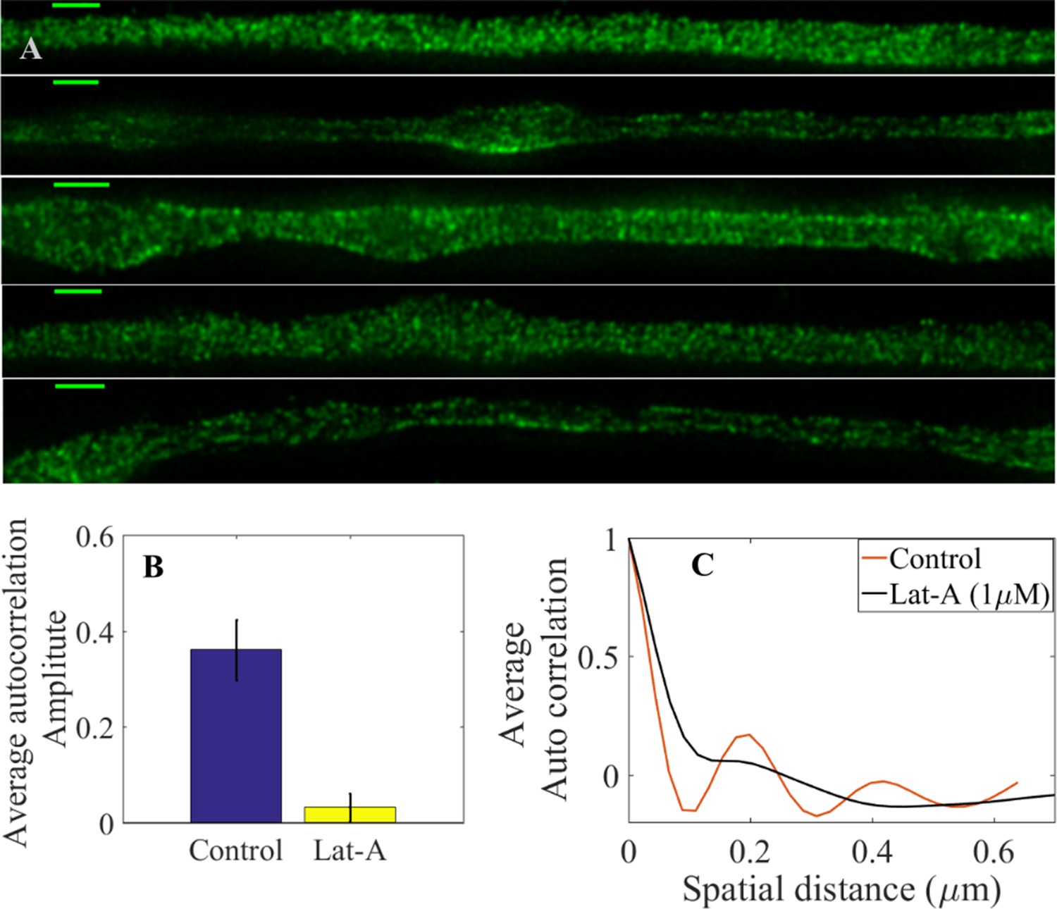
STED super resolution microscopy analysis of Lat-A-treated axons.
(A) Super-resolution images of 2-DIV axons treated for 30 min with 1 µM Lat-A labelled using primary antibody anti -II spectrin and secondary antibody anti-mouse IgG conjugated to Alexa Fluor 488 (Scale bar = 1 μm). It is clearly seen that the periodicity seen in control axons Figure 4—figure supplement 2 is absent in these images. (B) 1-D autocorrelation amplitude for several axon segments of 1 μm averaged over many axons (n = 10) which suggests that the spectrin periodicity is disrupted in Lat-A treated axons. (C) Intensity-intensity autocorrelation of DMSO vehicle control axons and those treated with Lat-A (1μM) for 30 min, averaged over many axons (n = 10). Vehicle control axons show a clear periodicity of ∼200 nm and strong correlation where as Lat-A treated axons show very weak correlation (see Material and methods for details).
Figure 4—figure supplement 5
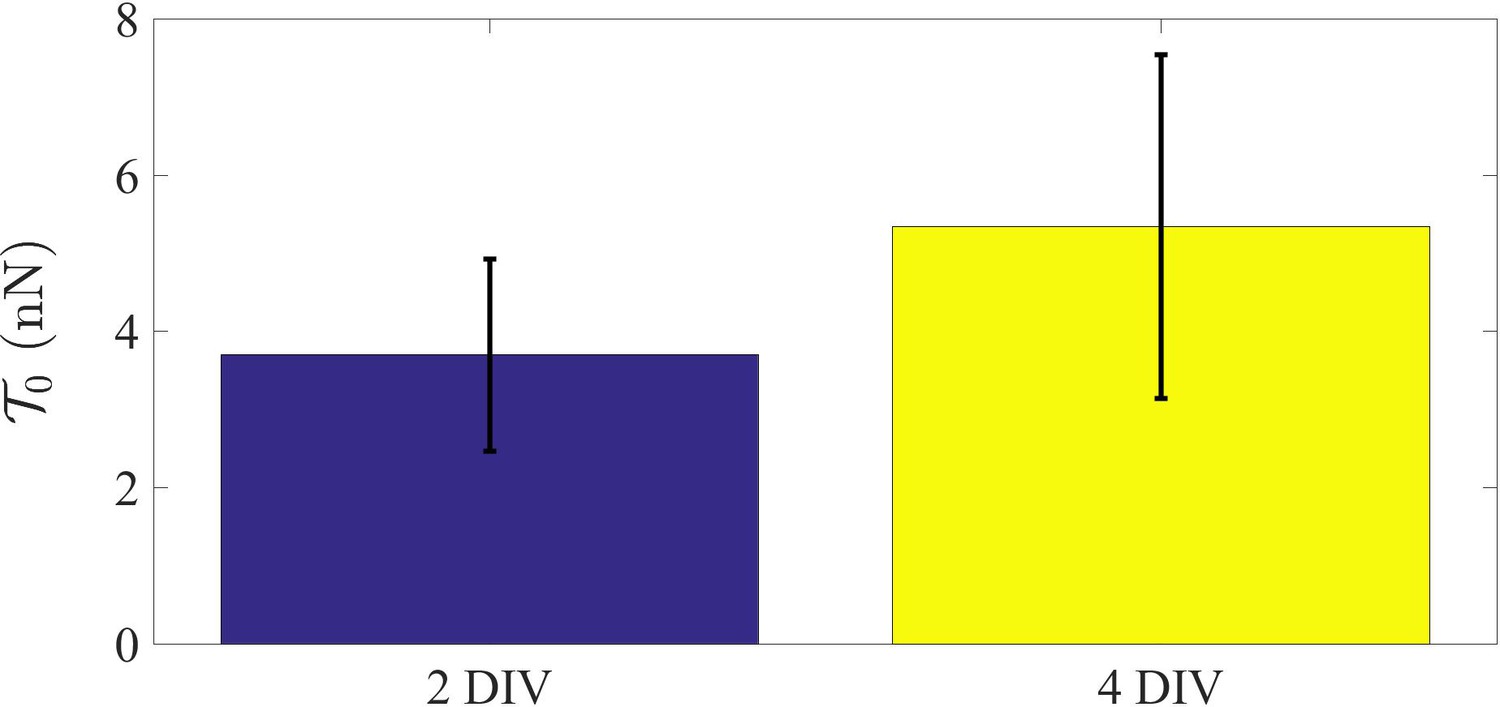
Rest tension variation with DIV.
Plot showing the difference in rest tension with age for 2-DIV and 4-DIV axons. 2-DIV: n = 10, mean = 3.7, SE = 1.2; 4-DIV: n = 7, mean = 5.3, SE = 2.2. Note that the actin-spectrin lattice becomes more prominent and extensive with DIV.
Figure 4—figure supplement 6
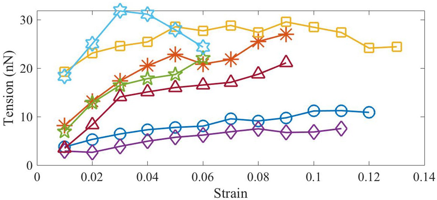
Steady state tension vs. strain in 4-DIV axons.
Evolution of the steady state tension as a function of strain for axons grown for four days in culture (4-DIV).
Figure 4—figure supplement 7
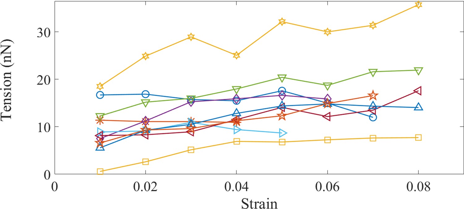
Non-averaged data for steady state tension vs. strain in control Morpholino axons.
Evolution of the steady state tension as a function of strain for control Morpholino treated axons.
Figure 5 with 4 supplements
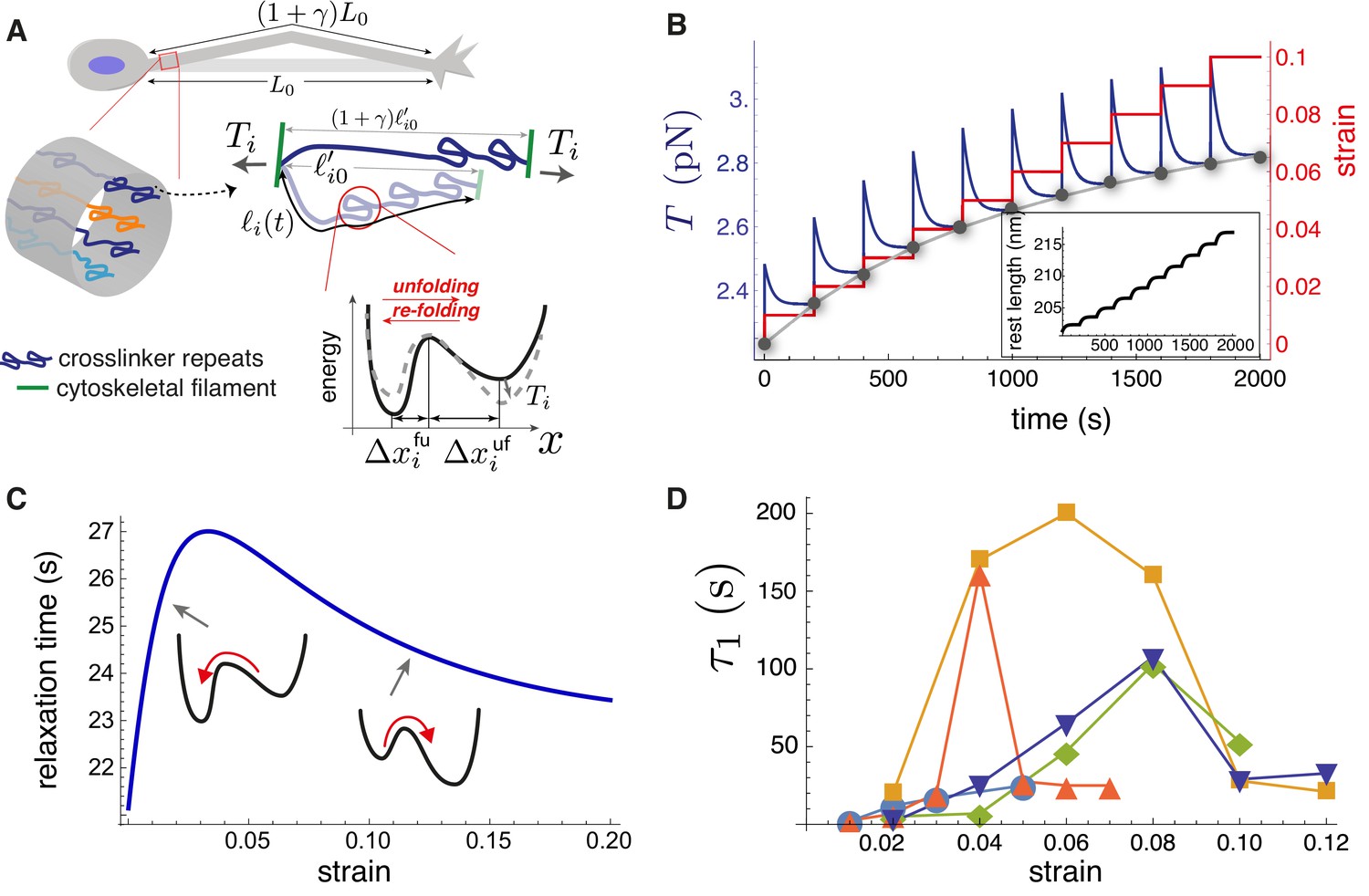
Theoretical model recapitulates strain-softening and tension relaxation.
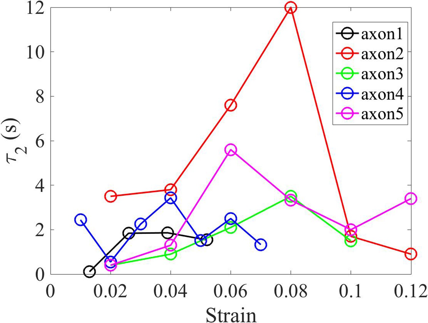
(A) Schematic illustration of a stretched axon, showing unfolding of a crosslinking protein repeat as an underlying tension relaxation mechanism. The axon, initially with length , is stretched to . In the model, any cylindrical portion of axon contains various crosslinking proteins (shown using different colors) that experience the strain . The contour length of the crosslinker between two cytoskeletal filaments, , is variable because of repeat unfolding and re-folding. This process is represented by an energy potential with two minima. The tension, , pushes the unfolded minimum down and the folded minimum up. (B) Model calculation for a single elastic element for multiple step-strain protocol. Tension versus time (purple) shows a jump after strain increment is applied (red), followed by relaxation to a steady-state value (gray points), passed through by the equilibrium tension versus extension curve "(gray)". This relaxation coincides with progressive repeat unfolding, as represented by the change in rest length (inset). (C) Tension relaxation after a small change in applied strain is exponential, with a relaxation time, , that depends non-monotonically on the strain. The inset cartoons are to show that is largely controlled by re-folding at low strain, and by unfolding at higher strain. (D) Fitting the tension relaxation data obtained from experiments like the one shown in Figure 2B to a function that is the sum of two exponentials (Figure 5—figure supplement 2, Figure 5—figure supplement 4) reveals a long relaxation time (denoted ) with a qualitatively similar dependence on strain as with the model (C) and a short relaxation time (Figure 5—figure supplement 3). Model calculations in B and C were done using the following parameters for spectrin: nm (Stokke et al., 1986), nm (Xu et al., 2013), nm, nm, nm, and nm. We also used s-1, s-1(Scott et al., 2004) and pN.nm.
Figure 5—figure supplement 1
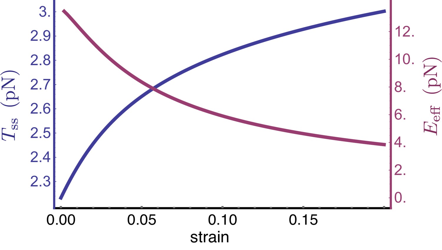
Model equilibrium tension and effective modulus vs.strain.
Model equilibrium tension, and effective Young’s modulus, versus strain curve for a single elastic element. The tension curve (blue) is obtained by solving Equations 2, 3, 4, 5 and 8 of the main text at equilibrium (). The Young’s modulus curve (purple) is obtained by taking , with the tension at zero strain, and dividing this quantity by the strain . The parameters used for both plots are values appropriate for spectrin tetramers: nm, nm, nm, nm, nm, and nm. We also used s-1, s-1, and pN.nm.
Figure 5—figure supplement 2
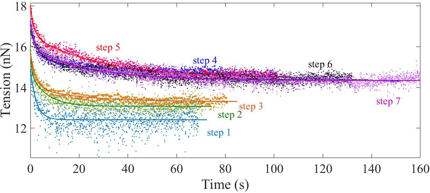
Double exponential fits of tension relaxation data.
Plots showing double exponential fits to the tension relaxation data from multi-step experiment (2-DIV axons) using where A, B, and C are positive constants and and are the two relaxation times.
Figure 5—figure supplement 3
Shorter relaxation time from double exponential fit.
Plot showing the short relaxation time () as a function of strain for different 2-DIV axons.
Figure 5—figure supplement 4
Normalized double exponential fits.
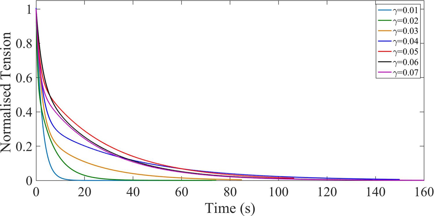
The fitted curves for tension relaxation after each step were normalized by the tension immediately after each step and plotted together to better illustrate the variation in relaxation time with step number. The normalized tension is calculated as , where is the axonal tension, is the peak value of tension for each step and is the steady state tension after the force has relaxed.
Tables
Key resources table
| Reagent type (species) or resource | Designation | Source or reference | Identifiers | Additional information |
|---|---|---|---|---|
| Genetic reagent | control MO | Standard control oligo, GeneTools | Gene Tools, LLC | 5’-CCTCTTACCTCAGTTACAATTTATA-3’ |
| Genetic reagent | Photo control MO | Standard control oligo, GeneTools | Gene Tools, LLC | 5’-CCTCTTACCTCAGTTACAATTTATA-3’ |
| Genetic reagent | Specific MO | Specific beta-II spectrin Gene tools | Gene Tools, LLC | 5’-GTCGCCACTGTTGTCGTCATC-3’ |
| Antibody | Beta-II spectrin antibody | BD biosciences | RRID:AB_399854 | (1:1500) |
| Antibody | anti-mouse Alexa Fluor 568 | Thermo Fisher Scientific | RRID:AB_2534072 | (1:1000) |
| Antibody | Anti-mouse Alexa Fluor 488 | Thermo Fisher Scientific | RRID:AB_2534069 | (1:1000) |
| Chemical compound, drug | Nocodazole | Sigma-Aldrich | M1404, Sigma-Aldrich | 10 μM |
| Chemical compound, drug | Latrunculin-A | Sigma-Aldrich | L5163, Sigma-Aldrich | 1 μM |
| Chemical compound, drug | Jasplakinolide | Thermo Fisher Scientific | J7473, Thermo Fisher Scientific | 5 μM |
| Chemical compound, drug | Paclitaxel (Taxol) | Sigma-Aldrich | T7402, Sigma-Aldrich | 10 μM |
| Chemical compound, drug | Blebbistatin | Sigma-aldrich | B0560, Sigma-Aldrich | 30 μM |
Appendix 1—table 1
STED Super Resolution Microscopy analysis of different DIV axons—STED image analysis for quantification of rings:
Here we quantify the occurrence of periodic rings (ladders) seen at various DIVs within an imaging field of view. It is evident from the table that as axon mature the rings develop all over the axons.
| DIV | No. of | Regular ladder | Ladder in patches | No visible ladder | |||
|---|---|---|---|---|---|---|---|
| Axons | Number | % | Number | % | Number | % | |
| 1 | 14 | 3 | 21.4 | 3 | 21.4 | 8 | 57.1 |
| 2 | 13 | 4 | 30.8 | 6 | 46.2 | 3 | 23.1 |
| 3 | 13 | 8 | 61.5 | 5 | 38.5 | 0 | 0 |
| 4 | 10 | 7 | 70.0 | 3 | 30.0 | 0 | 0 |
| 5 | 13 | 10 | 76.9 | 3 | 23.1 | 0 | 0 |
Appendix 1—table 2
Crosslink-detachment vs domain unfolding.
A summary of different scenario and their expected mechanical response.
| Model | Strain-softening of steady state moduli | Solid-like steady state | Peak in relaxation time vs strain | |
|---|---|---|---|---|
| i | Randomly crosslinked semiflexible polymer gel (Refs [Broedersz and MacKintosh, 2014]) | Initial entropic stiffening and subsequent softening due to force dependent crosslink detachment. Crosslink unbinding causes energy dissipation and stress relaxation. | Solid-like in stiffening regime and fluid-like in softening regime. | No |
| ii | Aligned microtubules with force dependent crosslinks (Refs [Ahmadzadeh et al., 2015; de Rooij and Kuhl, 2018]) | Can exhibit direct softening due to crosslink detachment as entropic effect is minimal. | Fluid-like at long times unless one invokes another parallel structure with permanent crosslinks. | No |
| iii | Force dependent unfolding and force dependent re-folding of spectrin domains. | Exhibits direct strain softening when spectrin is in fully extended configuration (as suggested by 190 nm tetramer spacing and FRET data) Dissipation and stress relaxation due to unfolding of domains. | Solid-like at long times as unfolded domains can take load unlike detached crosslinks. | Peak in relaxation time vs strain because unfolding rate increases with force while re-folding rate decreases with force. |
Additional files
Download links
A two-part list of links to download the article, or parts of the article, in various formats.
Downloads (link to download the article as PDF)
Open citations (links to open the citations from this article in various online reference manager services)
Cite this article (links to download the citations from this article in formats compatible with various reference manager tools)
The axonal actin-spectrin lattice acts as a tension buffering shock absorber
eLife 9:e51772.
https://doi.org/10.7554/eLife.51772


