SpikeForest, reproducible web-facing ground-truth validation of automated neural spike sorters
Figures
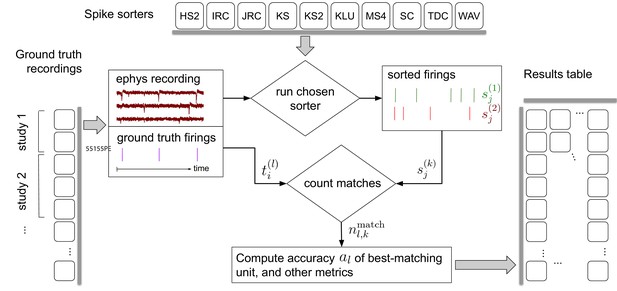
Simplified flow diagram of the SpikeForest analysis pipeline.
Each in a collection of spike sorting codes (top) are run on each recording with ground truth (left side) to yield a large matrix of sorting results and accuracy metrics (right). See the section on comparison with ground truth for mathematical notations. Recordings are grouped into ‘studies’, and those into ‘study sets’; these share features such as probe type and laboratory of origin. The web interface summarizes the results table by grouping them into study sets (as in Figure 2), but also allows drilling down to the single study and recording level. Aspects such as extraction of mean waveforms, representative firing events, and computation of per-unit SNR are not shown, for simplicity.
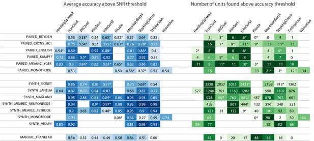
Main results table from the SpikeForest website showing aggregated results for 10 algorithms applied to 13 registered study sets.
The left columns of the table show the average accuracy (see (5)) obtained from averaging over all ground-truth units with SNR above an adjustable threshold, here set to 8. The right columns show the number of ground-truth units with accuracy above an adjustable threshold, here set to 0.8. The first five study sets contain paired recordings with simultaneous extracellular and juxta- or intra-cellular ground truth acquisitions. The next six contain simulations from various software packages. The SYNTH_JANELIA, obtained from Pachitariu et al., 2019, is simulated noise with realistic spike waveforms superimposed at known times. The last study set is a collection of human-curated tetrode data. An asterisk indicates an incomplete (timed out) or failed sorting on a subset of results; in these cases, missing accuracies are imputed using linear regression as described in the Materials and methods. Empty cells correspond to excluded sorter/study set pairs. These results reflect the analysis run of March 23rd, 2020.
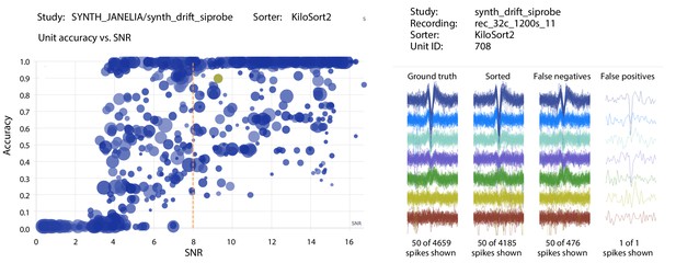
Screenshots from the SpikeForest website.
(left) Scatter plot of accuracy vs. SNR for each ground-truth unit, for a particular sorter (KiloSort2) and study (a simulated drift dataset from the SYNTH_JANELIA study set). The SNR threshold for the main table calculation is shown as a dashed line, and the user-selected unit is highlighted. Marker area is proportional to the number of events, and the color indicates the particular recording within the study. (right) A subset of spike waveforms (overlaid) corresponding to the selected ground truth unit, in four categories: ground truth, sorted, false negative, and false positive.
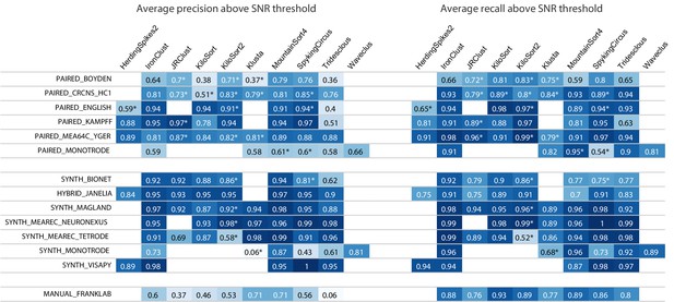
Results table from the SpikeForest website, similar to the left side of Figure 2 except showing aggregated precision and recall scores rather than accuracy.
Precision measures how well the algorithm avoids false positives, whereas recall is the complement of the false negative rate. An asterisk indicates an incomplete (timed out) or failed sorting on a subset of results; in these cases, missing accuracies are imputed using linear regression as described in the Materials and methods. Empty cells correspond to excluded sorter/study set pairs. These results reflect the analysis run of March 23rd, 2020.
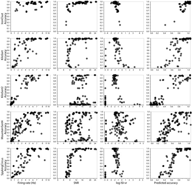
Relationship between ground-truth accuracy and three quality metrics for all sorted units (with SNR ≥5), for the SYNTH_JANELIA tetrode study and five spike sorting algorithms.
Each marker represents a sorted unit. The x-axis of the plots in the final column is the predicted accuracy via linear regression using all three predictors (SNR, firing rate, and log ISI-vr).

Interaction of software and hardware components of the SpikeForest system, showing the flow of data from the server-side analysis (left) to the user’s web browser (right).
The processing pipeline automatically detects which sorting jobs need to be updated and runs these in parallel as needed on a compute cluster. Processing results are uploaded to two databases, one for relatively small JSON files and the other for large binary content. A NodeJS application pulls data from these databases in order to show the most up-to-date results on the front-end website.
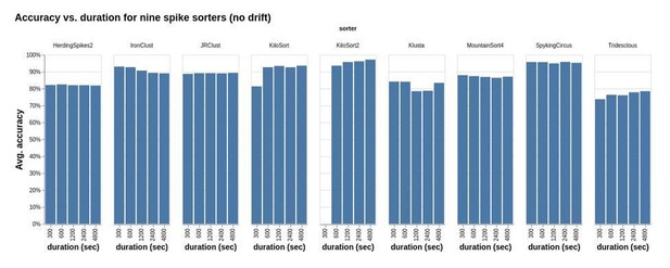
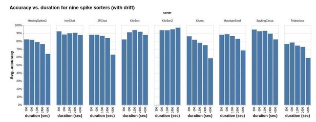
Accuracy vs. duration for nine sorters applied to a study set of simulated recordings.
Tables
Table of spike sorting algorithms currently included in the SpikeForest analysis.
Each algorithm is registered into the system via a Python wrapper. A Docker recipe defines the operating system and environment where the sorter is run. Algorithms with asterisks were updated and optimized using SpikeForest data. For the other algorithms, we used the default or recommended parameters.
| Sorting algorithm | Language | Notes |
|---|---|---|
| HerdingSpikes2* | Python | Designed for large-scale, high-density multielectrode arrays. See Hilgen et al., 2017. |
| IronClust* | MATLAB and CUDA | Derived from JRCLUST. See Jun et al., in preparation. |
| JRCLUST | MATLAB and CUDA | Designed for high-density silicon probes. See Jun et al., 2017a. |
| KiloSort | MATLAB and CUDA | Template matching. See Pachitariu et al., 2016. |
| KiloSort2 | MATLAB and CUDA | Derived from KiloSort. See Pachitariu et al., 2019. |
| Klusta | Python | Expectation-Maximization masked clustering. See Rossant et al., 2016. |
| MountainSort4 | Python and C++ | Density-based clustering via ISO-SPLIT. See Chung et al., 2017. |
| SpyKING CIRCUS* | Python and MPI | Density-based clustering and template matching. See Yger et al., 2018. |
| Tridesclous* | Python and OpenCL | See Garcia and Pouzat, 2019. |
| WaveClus | MATLAB | Superparamagnetic clustering. See Chaure et al., 2018; Quiroga et al., 2004. |
Table of study sets currently included in the SpikeForest analysis.
Study sets fall into three categories: paired, synthetic, and curated. Each study set comprises one or more studies, which in turn comprise multiple recordings acquired or generated under the same conditions.
| Study set | # Rec. / # Elec. / Dur. | Source lab. | Description |
|---|---|---|---|
| Paired intra/extracellular | |||
| PAIRED_BOYDEN | 19 / 32ch / 6-10min | E. Boyden | Subselected from 64, 128, or 256-ch. probes, mouse cortex |
| PAIRED_CRCNS_HC1 | 93 / 4-6ch / 6-12min | G. Buzsaki | Tetrodes or silicon probe (one shank) in rat hippocampus |
| PAIRED_ENGLISH | 29 / 4-32ch / 1-36min | D. English | Hybrid juxtacellular-Si probe, behaving mouse, various regions |
| PAIRED_KAMPFF | 15 / 32ch / 9-20min | A. Kampff | Subselected from 374, 127, or 32-ch. probes, mouse cortex |
| PAIRED_MEA64C_YGER | 18 / 64ch / 5min | O. Marre | Subselected from 252-ch. MEA, mouse retina |
| PAIRED_MONOTRODE | 100 / 1ch / 5-20min | Boyden, Kampff, Marre, Buzsaki | Subselected from paired recordings from four labs |
| Simulation | |||
| SYNTH_BIONET | 36 / 60ch / 15min | AIBS | BioNet simulation containing no drift, monotonic drift, and random jumps; used by JRCLUST, IronClust |
| SYNTH_JANELIA | 60 / 4-64ch / 5-20min | M. Pachitariu | Distributed with KiloSort2, with and without simulated drift |
| SYNTH_MAGLAND | 80 / 8ch / 10min | Flatiron Inst. | Synthetic waveforms, Gaussian noise, varying SNR, channel count and unit count |
| SYNTH_MEAREC_NEURONEX | 60 / 32ch / 10min | A. Buccino | Simulated using MEAREC, varying SNR and unit count |
| SYNTH_MEAREC_TETRODE | 40 / 4ch / 10min | A. Buccino | Simulated using MEAREC, varying SNR and unit count |
| SYNTH_MONOTRODE | 111 / 1ch / 10min | Q. Quiroga | Simulated by Quiroga lab by mixing averaged real spike waveforms |
| SYNTH_VISAPY | 6 / 30ch / 5min | G. Einevoll | Generated using VISAPy simulator |
| Human curated | |||
| MANUAL_FRANKLAB | 21 / 4ch / 10-40min | L. Frank | Three manual curations of the same recordings |


