A connectome and analysis of the adult Drosophila central brain
- Janelia Research Campus, Howard Hughes Medical Institute, United States
- Google Research, United States
- Life Sciences Centre, Dalhousie University, Canada
- Google Research, Google LLC, Switzerland
- Institute for Quantitative Biosciences, University of Tokyo, Japan
- MRC Laboratory of Molecular Biology, United States
- Institute of Zoology, Biocenter Cologne, University of Cologne, Germany
- Department of Zoology, University of Cambridge, United Kingdom
Figures
Figure 1
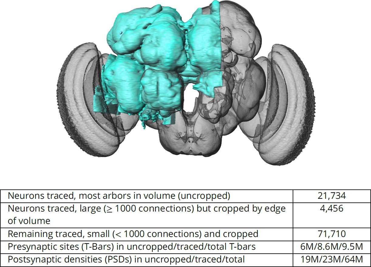
The hemibrain and some basic statistics.
The highlighted area shows the portion of the central brain that was imaged and reconstructed, superimposed on a grayscale representation of the entire Drosophila brain. For the table, a neuron is traced if all its main branches within the volume are reconstructed. A neuron is considered uncropped if most arbors (though perhaps not the soma) are contained in the volume. Others are considered cropped. Note: (1) our definition of cropped is somewhat subjective; (2) the usefulness of a cropped neuron depends on the application; and (3) some small fragments are known to be distinct neurons. For simplicity, we will often state that the hemibrain contains ≈25K neurons.
Figure 2
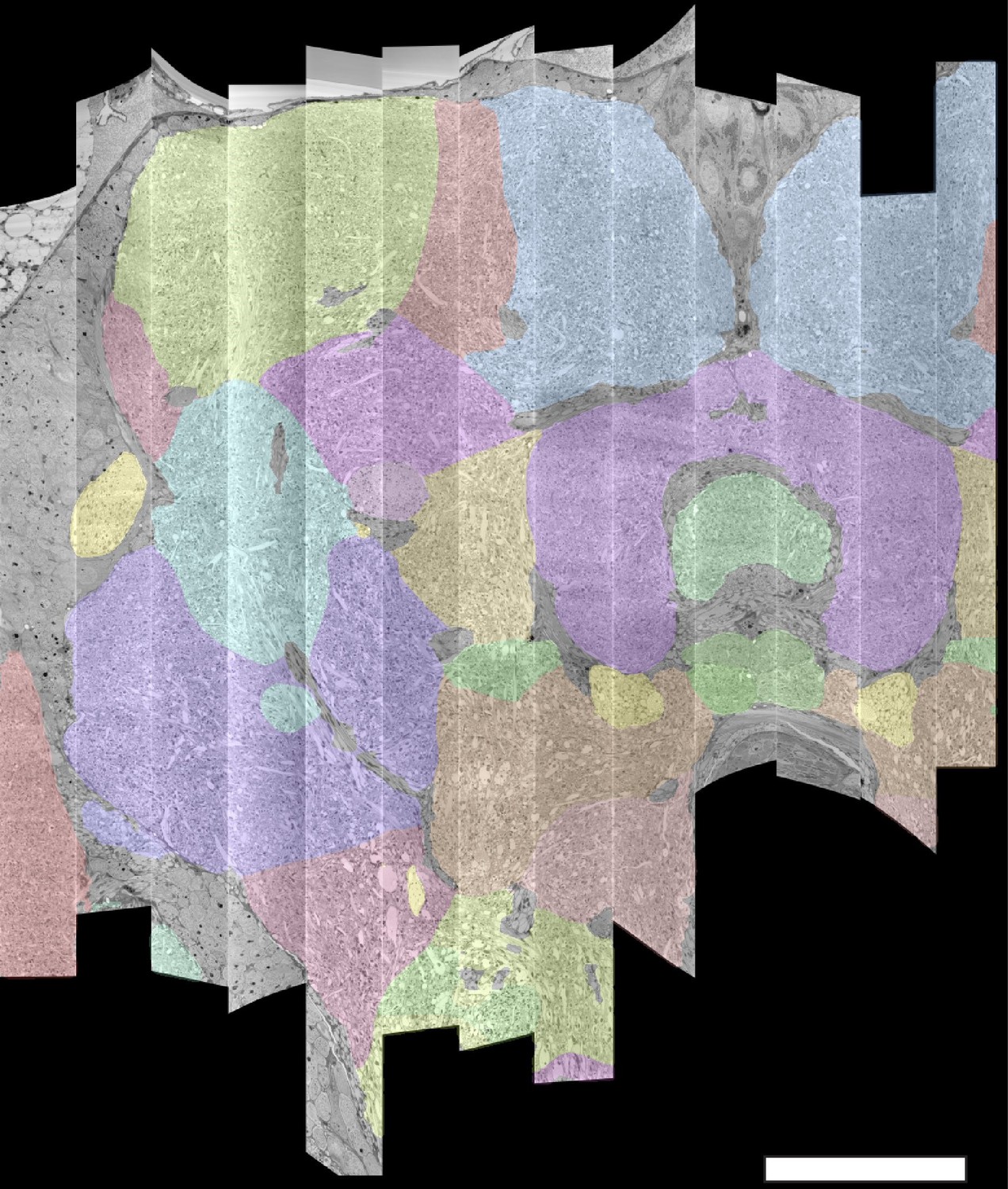
The 13 slabs of the hemibrain, each flattened and co-aligned.
A vertical section at the level of the fan-shaped body is shown. Colors are arbitrary and added to the monochrome data to show brain regions, as defined below. Scale bar 50 μm.
Figure 3
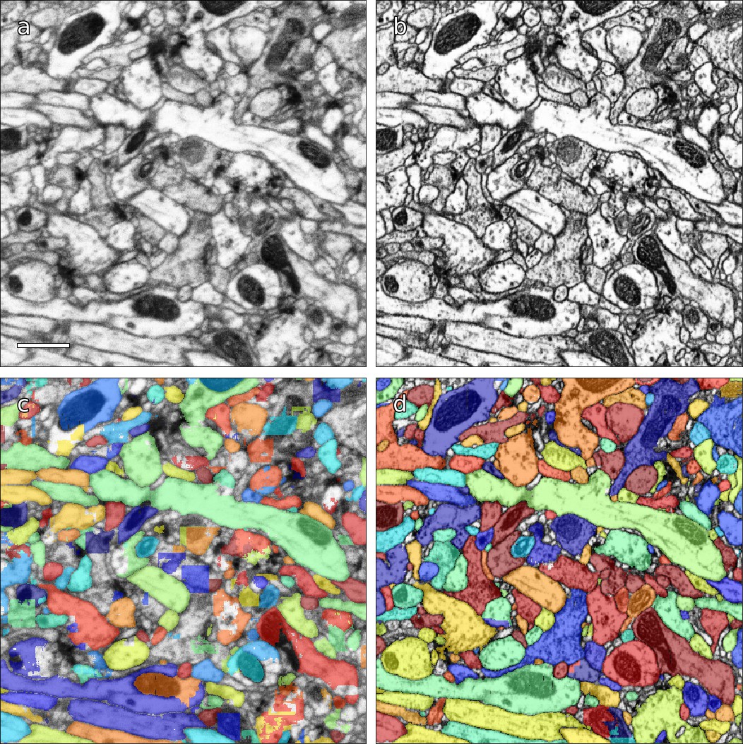
Examples of results of CycleGAN processing.
(a) Original EM data from tab 34 at a resolution of 16 nm / resolution, (b) EM data after CycleGAN processing, (c–d) FFN segmentation results with the 16 nm model applied to original and processed data, respectively. Scale bar in (a) represents 1 μm.
Figure 4
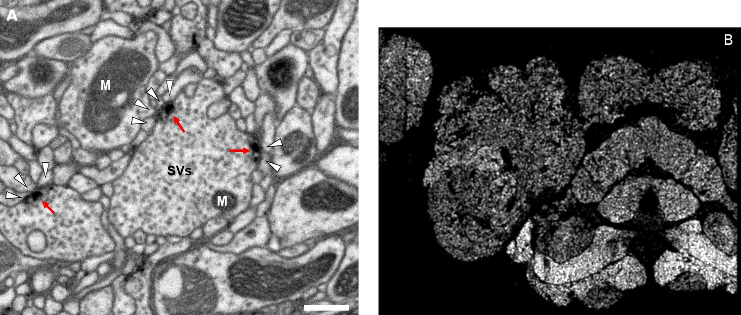
Well-preserved membranes, darkly stained synapses, and smooth round neurite profiles are characteristics of the hemibrain sample.
Panel (A) shows polyadic synapses, with a red arrow indicating the presynaptic T-bar, and white triangles pointing to the PSDs. We identified in total 64 million PSDs and 9.5 million T-bars in the hemibrain volume (Figure 1). Thus the average number of PSDs per T-bar in our sample is 6.7. Mitochondria (‘M’), synaptic vesicles (‘SV’), and the scale bar (0.5 μm) are shown. Panel (B) shows a horizontal cross section through a point cloud of all detected synapses. This EM point cloud defines many of the compartments in the fly’s brain, much like an optical image obtained using antibody nc82 (an antibody against Bruchpilot, a component protein of T-bars) to stain synapses. This point cloud is used to generate the transformation from our sample to the standard Drosophila brain.
Figure 5
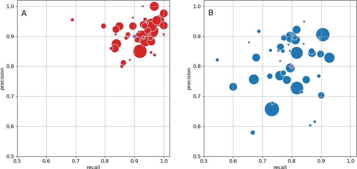
Precision and recall for synapse prediction, panel (A) for T-bars, and panel (B) for synapses as a whole including the identification of PSDs.
T-bar identification is better than PSD identification since this organelle is both more distinct and typically occurs in larger neurites. Each dot is one brain region. The size of the dot is proportional to the volume of the region. Humans proofreaders typically achieve 0.9 precision/recall on T-bars and 0.8 precision/recall on PSDs, indicated in purple. Data available in Figure 5—source datas 1–2.
-
Figure 5—source data 1
Data for Figure 5A.
Column A: precision; column B: recall; column C: region size.
- https://cdn.elifesciences.org/articles/57443/elife-57443-fig5-data1-v4.csv
-
Figure 5—source data 2
Data for Figure 5B.
Column A: precision; column B: recall; column C: region size.
- https://cdn.elifesciences.org/articles/57443/elife-57443-fig5-data2-v4.csv
Figure 6
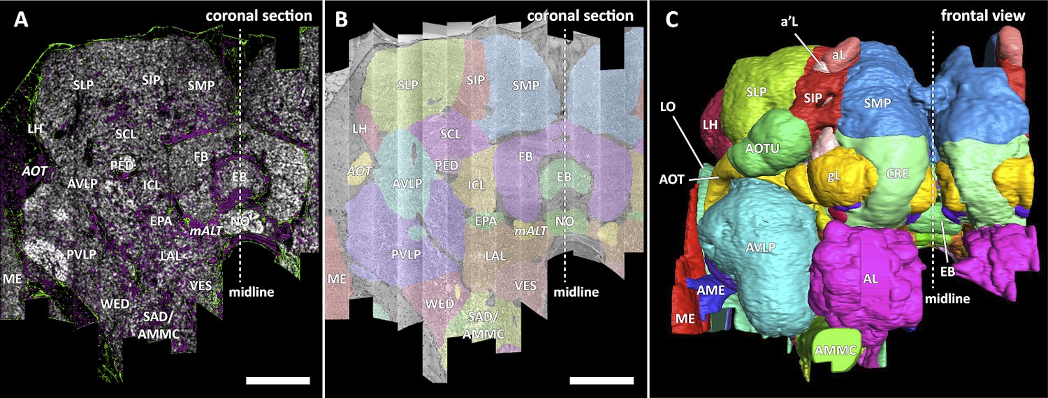
Division of the sample into brain regions.
(A) A vertical section of the hemibrain dataset with synapse point clouds (white), predicted glial tissue (green), and predicted fiber bundles (magenta). (B) Grayscale image overlaid with segmented neuropils at the same level as (A). (C) A frontal view of the reconstructed neuropils. Scale bar: (A, B) 50 μm.
Figure 7
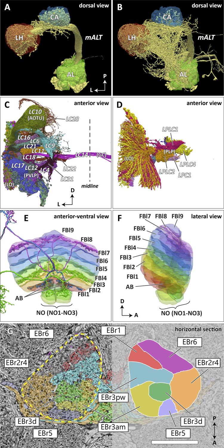
Reconstructed brain regions and substructures.
(A, B) Dorsal views of the olfactory projection neurons (PNs) and the innervated neuropils, AL, CA, and LH. Uniglomerular PNs projecting through the mALT are shown in (A), and multiglomerular PNs are shown in (B). (C, D) Columnar visual projection neurons. Each subtype of cells is color coded. LC cells are shown in (C), and LPC, LLPC, and LPLC cells are shown in (D). (E, F) The nine layers of the fan-shaped body (FB), along with the asymmetrical bodies (AB) and the noduli (NO), displayed as an anterior-ventral view (E), and a lateral view (F). In (E), three FB tangential cells (FB1D (blue), FB3A (green), FB8H (purple)) are shown as markers of the corresponding layers (FBl1, FBl3, and FBl8, respectively). (G) Zones in the ellipsoid body (EB) defined by the innervation patterns of different types of ring neurons. In this horizontal section of the EB, the left side shows the original grayscale data, and the seven ring neuron zones (see Table 1) are color-coded. The right side displays the seven segmented zones based on the innervation pattern, in a slightly different section. Scale bar: 20 μm.
Figure 8
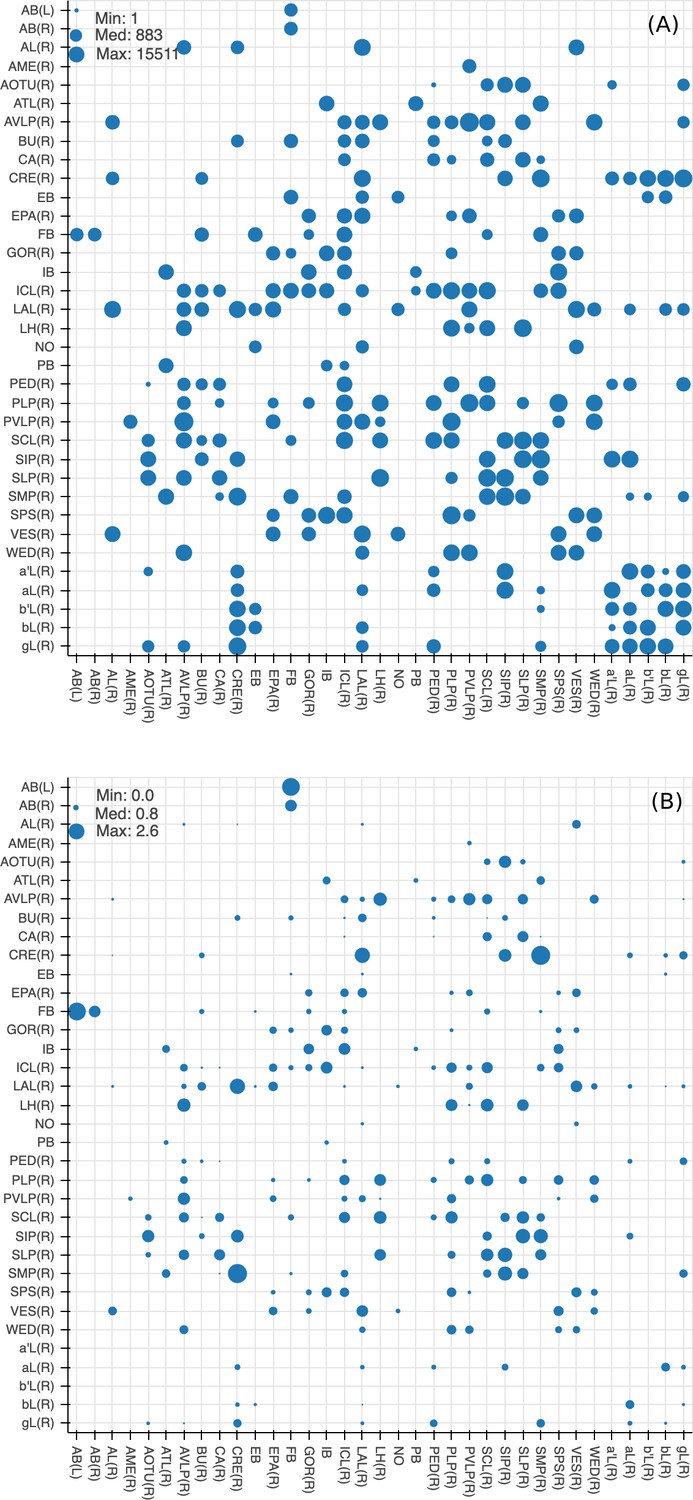
Quality checks of the brain compartments.
(A) Areas of the boundaries (in square microns) between adjacent neuropils, indicated on a log scale. (B) The number of excess crossings normalized by the area of neuropil boundary. Larger dots indicate a more uncertain boundary. Data available in Figure 8—source data 1.
-
Figure 8—source data 1
Data for Figure 8.
Column A: index number; column B: first ROI name; column C: second ROI name; column D: boundary area in square microns; column E: number of neurons crossings; column F: number of distinct neurons that cross; column G: (crossings - number of neurons) per area.
- https://cdn.elifesciences.org/articles/57443/elife-57443-fig8-data1-v4.csv
Figure 9
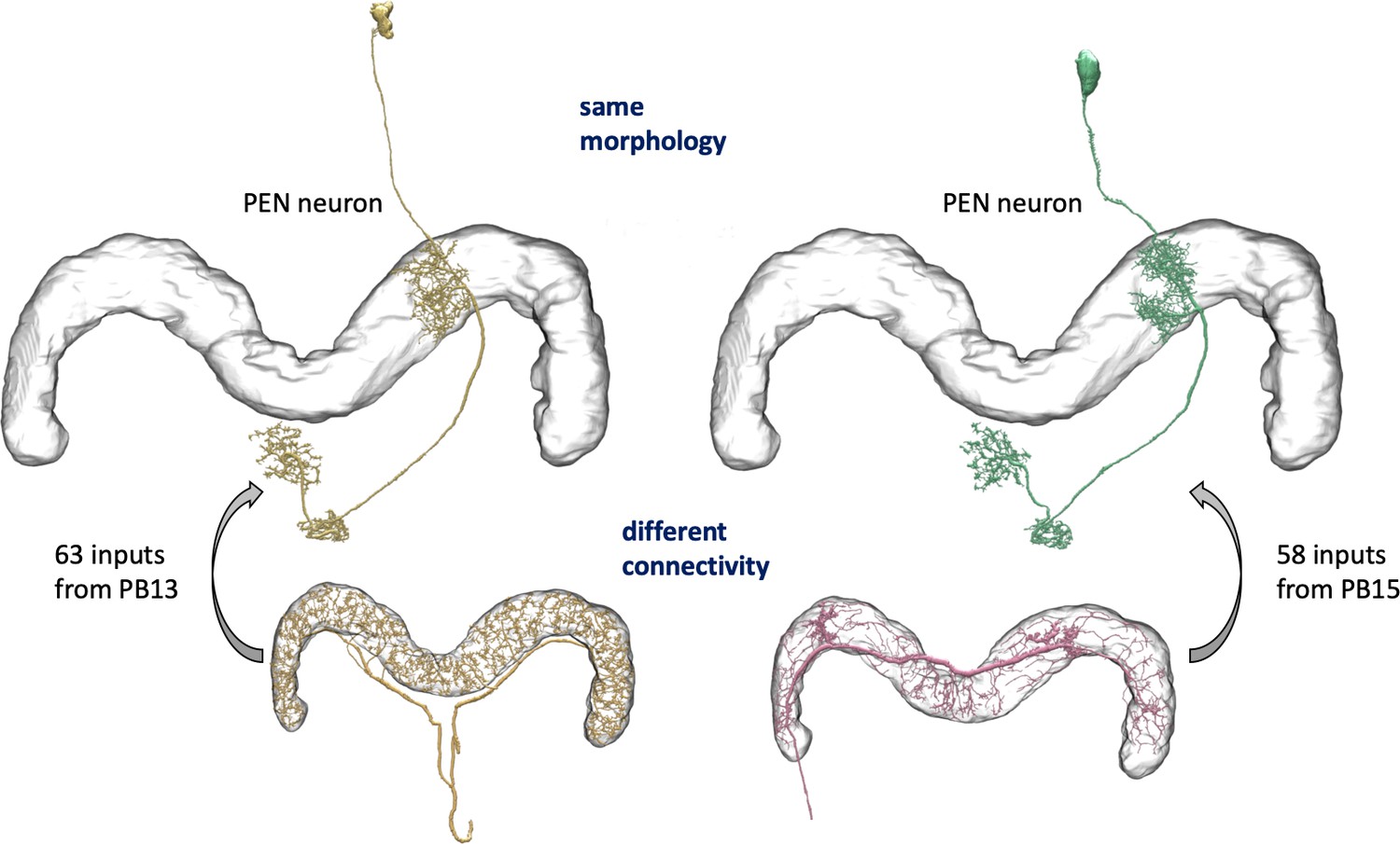
An example of two neurons with very similar shapes but differing connectivities.
PEN1 is on the left, PEN2 on the right.
Figure 10
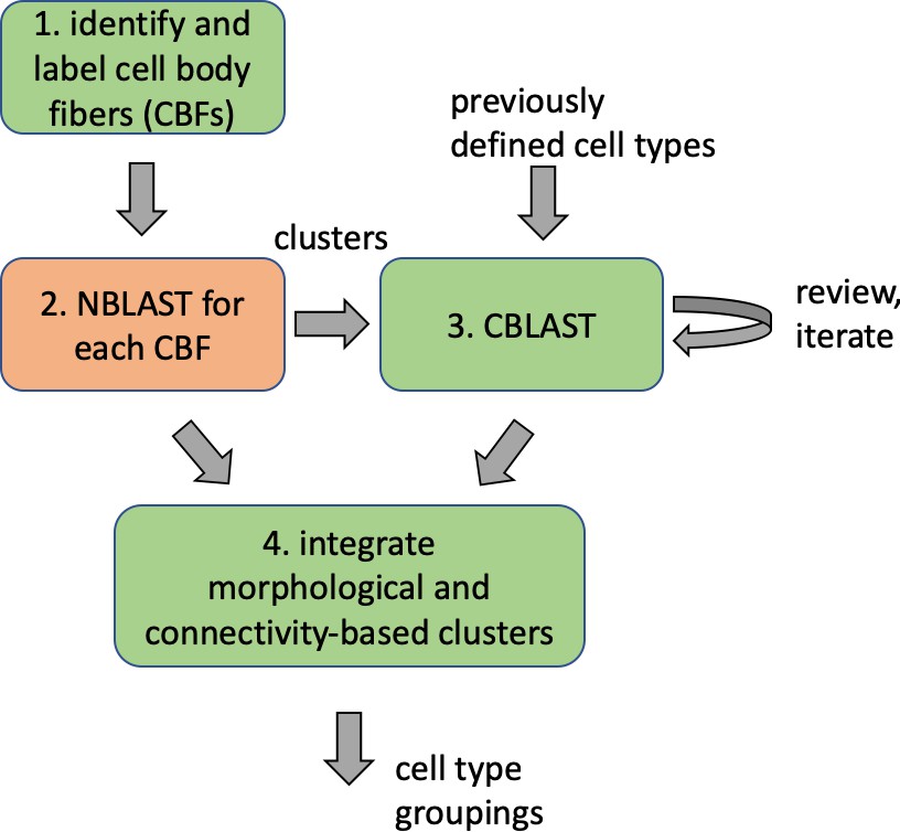
Workflow for defining cell types.
Figure 11
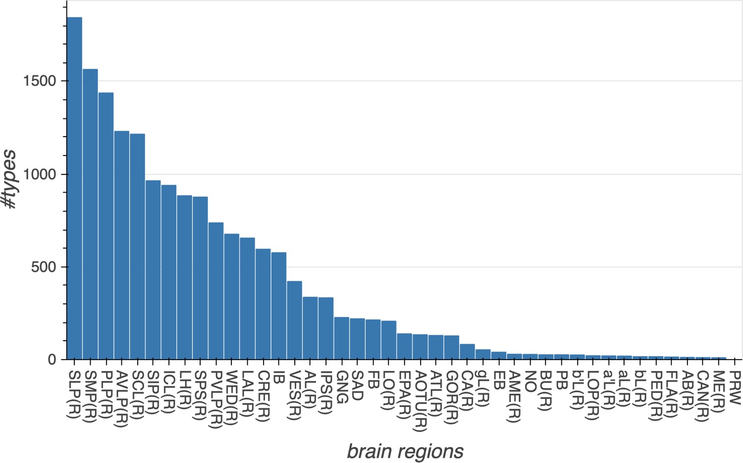
The number of cell types in each major brain region.
The total number of cell types shown in this graph is larger than the total number of cell types shown in Table 3, because types that arborize in multiple regions are counted in each region in which they occur. Data available in Figure 11—source data 1.
-
Figure 11—source data 1
Data for Figure 11.
Column A: region name; column B: number of cell types.
- https://cdn.elifesciences.org/articles/57443/elife-57443-fig11-data1-v4.csv
Figure 12
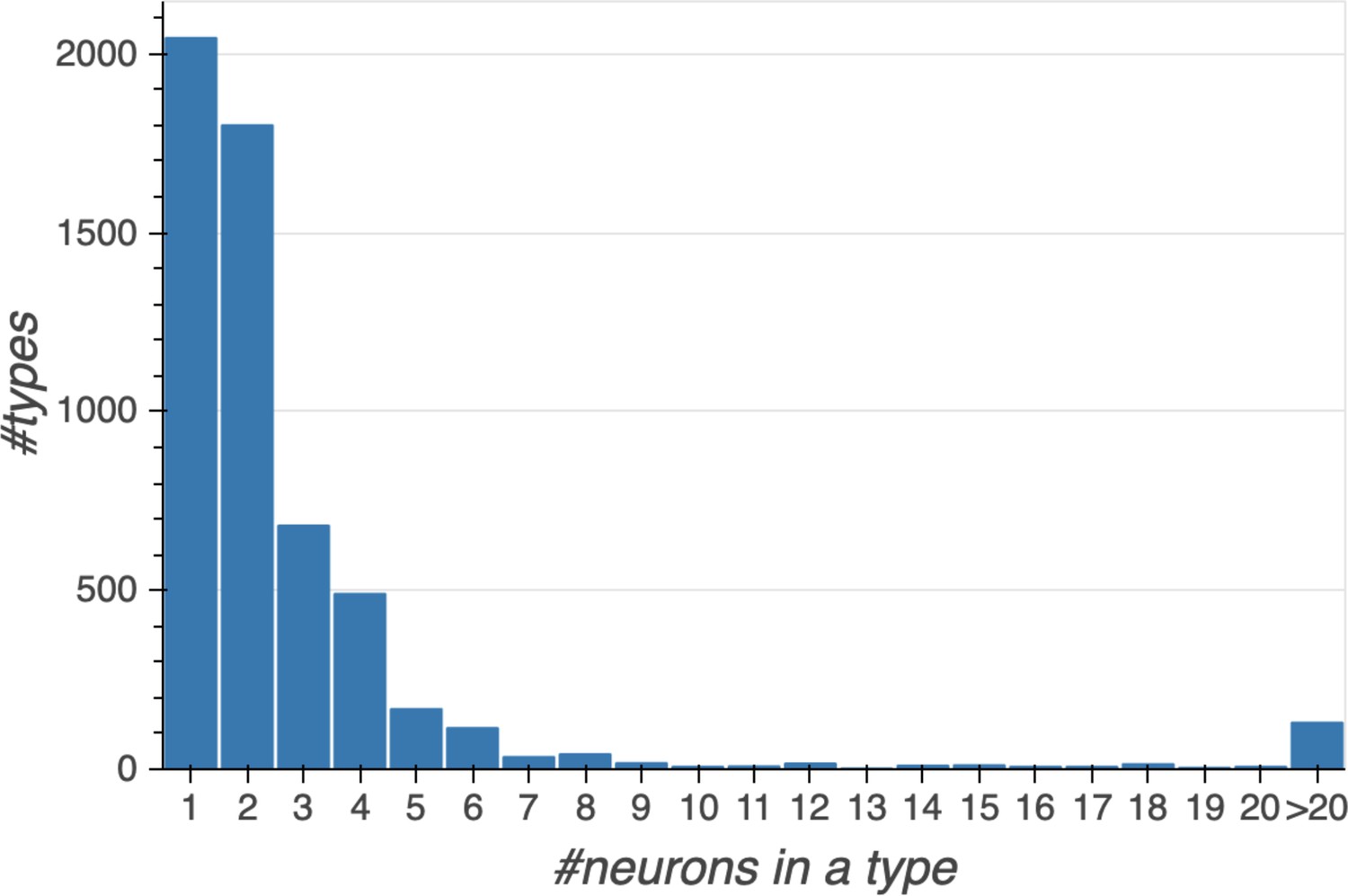
Histogram showing the number of cell types with a given number of constituent cells.
Data available in Figure 12—source data 1.
-
Figure 12—source data 1
Data for Figure 12.
Column A: number of instances of a cell; column B: Number of cell types with that number of instances.
- https://cdn.elifesciences.org/articles/57443/elife-57443-fig12-data1-v4.csv
Figure 13
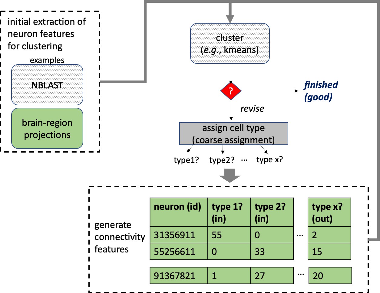
Overview of the operation of CBLAST.
Figure 14
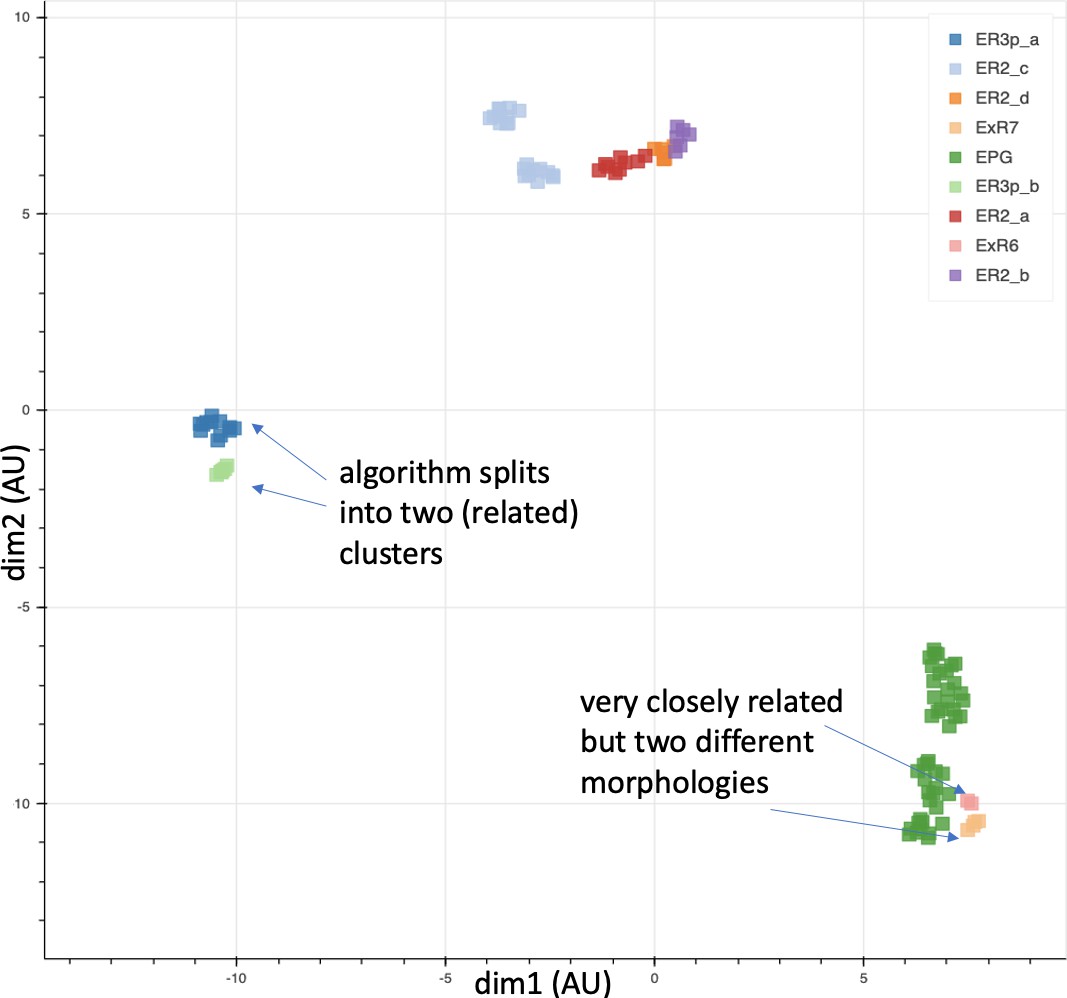
Cells of nine types plotted according to their connectivities.
Coordinates are in arbitrary units after dimensionality reduction using UMAP (McInnes et al., 2018). The results largely agree with those from morphological clustering but in some cases show separation even between closely related types.
Figure 15
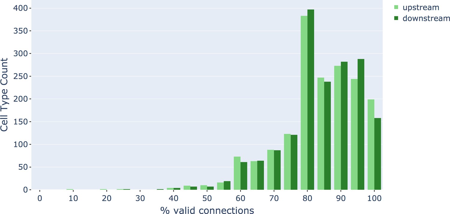
Connection precision of upstream and downstream partners for ≈1000 cell types.
Data available in Figure 15—source data 1.
-
Figure 15—source data 1
Data on 1735 neurons, one per row.
The histograms shown are computed from the columns 'final upstream perc' and 'final downstream perc'.
- https://cdn.elifesciences.org/articles/57443/elife-57443-fig15-data1-v4.csv
Figure 16
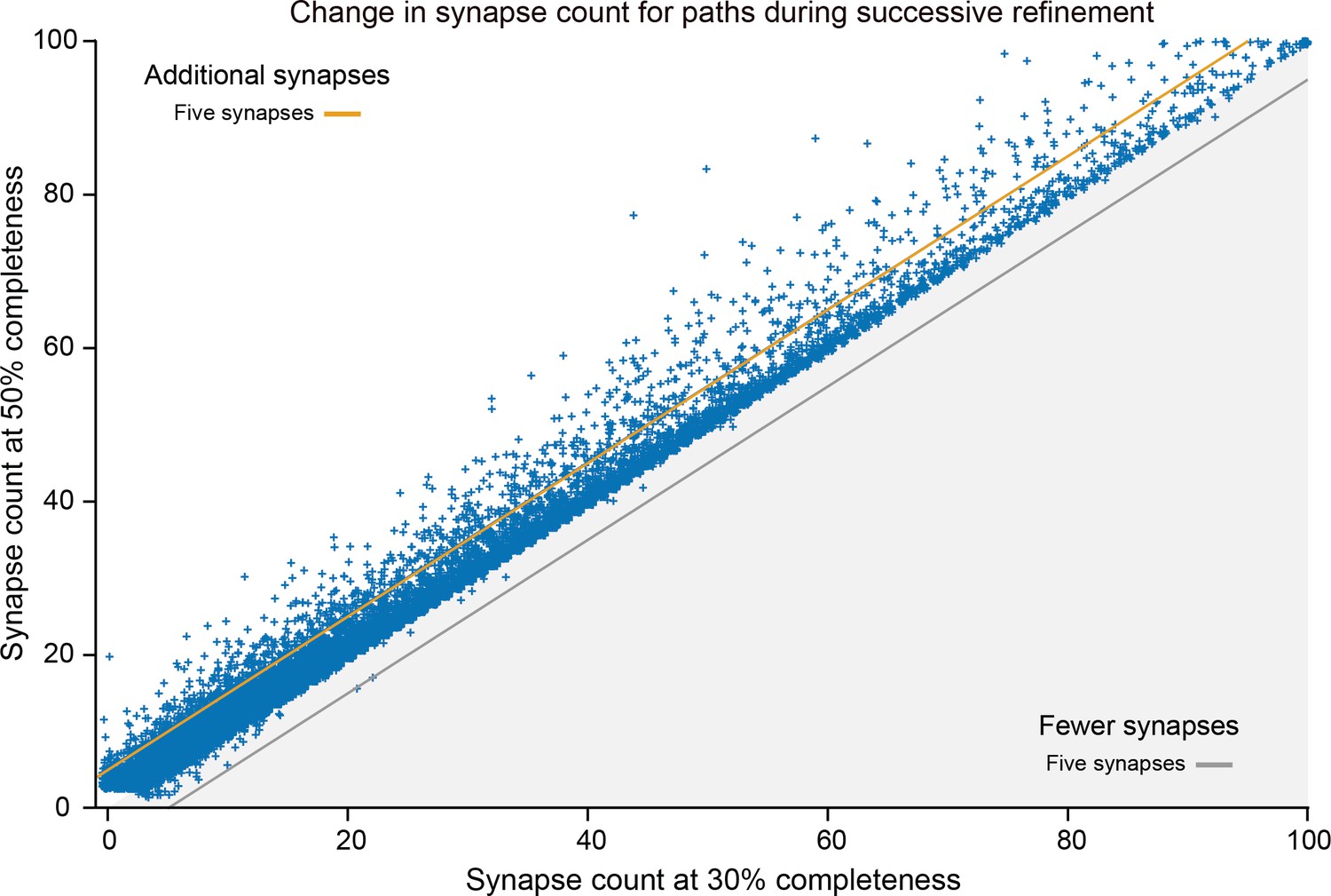
Difference between synapse counts in connections of the Ellipsoid Body, with increased completeness in proofreading.
Roughly 40,000 connection strengths are shown. Almost all points fall above the line Y = X, showing that almost all connections increased in synapse count, with very few decreasing. In particular, no path decreased by more than five synapses. Only two new strong (count >10) paths were found that were not present in the original. As proofreading proceeds, this error becomes less and less common since neuron fragments (orphans) are added in order of decreasing size (see text). Data available in Figure 16—source data 1.
-
Figure 16—source data 1
Data for Figure 16.
The first column is the synapse count before the additional proofreading, the second after. Each point includes a small random component so the points do not directly overlap.
- https://cdn.elifesciences.org/articles/57443/elife-57443-fig16-data1-v4.txt
Figure 17
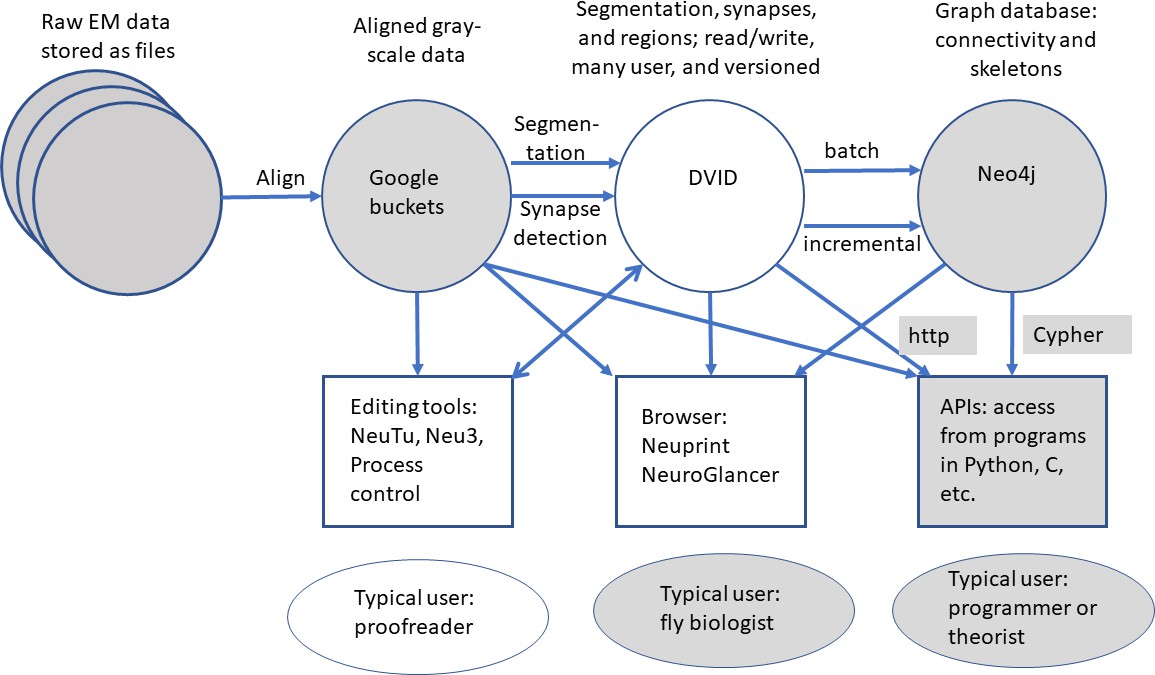
Overview of data representations of our reconstruction.
Circles are stored data representations, rectangles are application programs, ellipses represent users, and arrows indicate the direction of data flow labeled with transformation and/or format. Filled areas represent existing technologies and techniques; open areas were developed for the express purpose of EM reconstruction of large circuits.
Figure 18
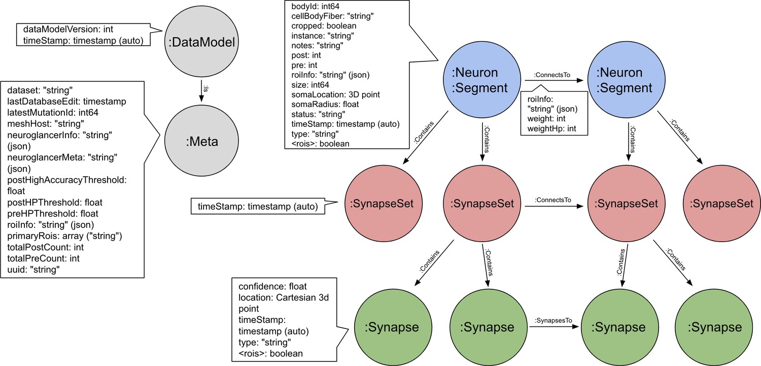
Schema for the neo4j graph model of the hemibrain.
Each neuron contains 0 or more SynapseSets, each of which contains one or more synapses. All the synapses in a SynapseSet connect the same two neurons. If the details of the synapses are not needed, the neuron-to-neuron weight can be obtained as a property on the ‘ConnectsTo’ relation, as can the distribution of this weight across different brain regions (the roiInfo).
Figure 19

Comparison of the size and orientation of brain images.
Sagittal section images at the plane of the mushroom body pedunculus are shown. Parallel lines indicate the direction of serial sectioning. Purple dotted lines indicate the axes of the pedunculus to show the sample orientation. Numbers indicate the angles of the pedunculus axes relative to the horizontal axis. Scale bar: 50 μm for all images. CA: calyx of the mushroom body. Panel (a) Hemibrain EM image stack. Grayscale indicates the density of the points of the presynaptic T-bars (point clouds). (b) Confocal light microscopy image stack provided by the Insect Brain Name Working Group (Ito et al., 2014), of a female brain mounted in 80% glycerol after antibody labeling. Presynaptic sites are labeled by GFP fused with the synaptic vesicle-associated protein neuronal synaptobrevin (nSyb), driven by the pan-neuronal expression driver line elav-GAL4 C155. (c) JRC2018 Unisex brain template (Bogovic et al., 2020), which is an average of 36 female and 26 male brains mounted in DPX plastic after dehydration with ethanol and clearization with xylene. Presynaptic sites are labeled with the SNAP chemical tag knock-in construct inserted into the genetic locus of the active zone protein bruchpilot (brp). The relative sizes of the brains, measured as the height along the lines that are perpendicular to the pedunculus axes, are 100:83:70 for (a), (b), and (c). These differences in size and orientation must be taken into account when comparing the sections and reconstructed neurons of the hemibrain EM and registered light microscopy images.
Figure 20
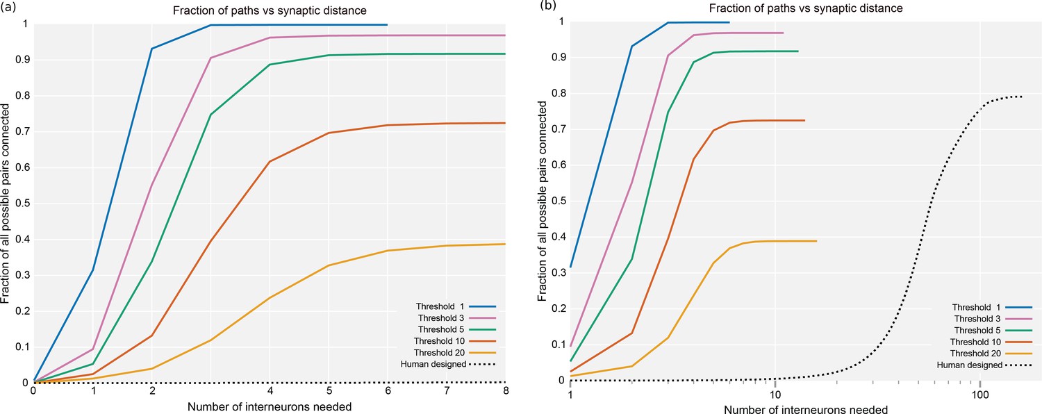
Plots of the percentage of pairs connected (of all possible) versus the number of interneurons required.
(a) It shows the data from the whole hemibrain, for up to eight interneurons. (b) It is a much wider view of the same data, shown on a log scale so the curve from a human designed system is visible. Data available in Figure 20—source datas 1–6.
-
Figure 20—source data 1
Data for threshold 1 trace.
The first column is the path length between two nodes, the second the number of pairs for which that is the length of the shortest path between them, and the third the cumulative fraction of all paths of that length or less.
- https://cdn.elifesciences.org/articles/57443/elife-57443-fig20-data1-v4.txt
-
Figure 20—source data 2
Data for threshold 3.
The first column is the path length between two nodes, the second the number of pairs for which that is the length of the shortest path between them, and the third the cumulative fraction of all paths of that length or less.
- https://cdn.elifesciences.org/articles/57443/elife-57443-fig20-data2-v4.txt
-
Figure 20—source data 3
Data for threshold 5 trace.
The first column is the path length between two nodes, the second the number of pairs for which that is the length of the shortest path between them, and the third the cumulative fraction of all paths of that length or less.
- https://cdn.elifesciences.org/articles/57443/elife-57443-fig20-data3-v4.txt
-
Figure 20—source data 4
Data for threshold 10 trace.
The first column is the path length between two nodes, the second the number of pairs for which that is the length of the shortest path between them, and the third the cumulative fraction of all paths of that length or less.
- https://cdn.elifesciences.org/articles/57443/elife-57443-fig20-data4-v4.txt
-
Figure 20—source data 5
Data for threshold 20 trace.
The first column is the path length between two nodes, the second the number of pairs for which that is the length of the shortest path between them, and the third the cumulative fraction of all paths of that length or less.
- https://cdn.elifesciences.org/articles/57443/elife-57443-fig20-data5-v4.txt
-
Figure 20—source data 6
Data for human designed trace.
The first column is the path length between two nodes, the second the number of pairs for which that is the length of the shortest path between them, and the third the cumulative fraction of all paths of that length or less.
- https://cdn.elifesciences.org/articles/57443/elife-57443-fig20-data6-v4.mm.txt
Figure 21
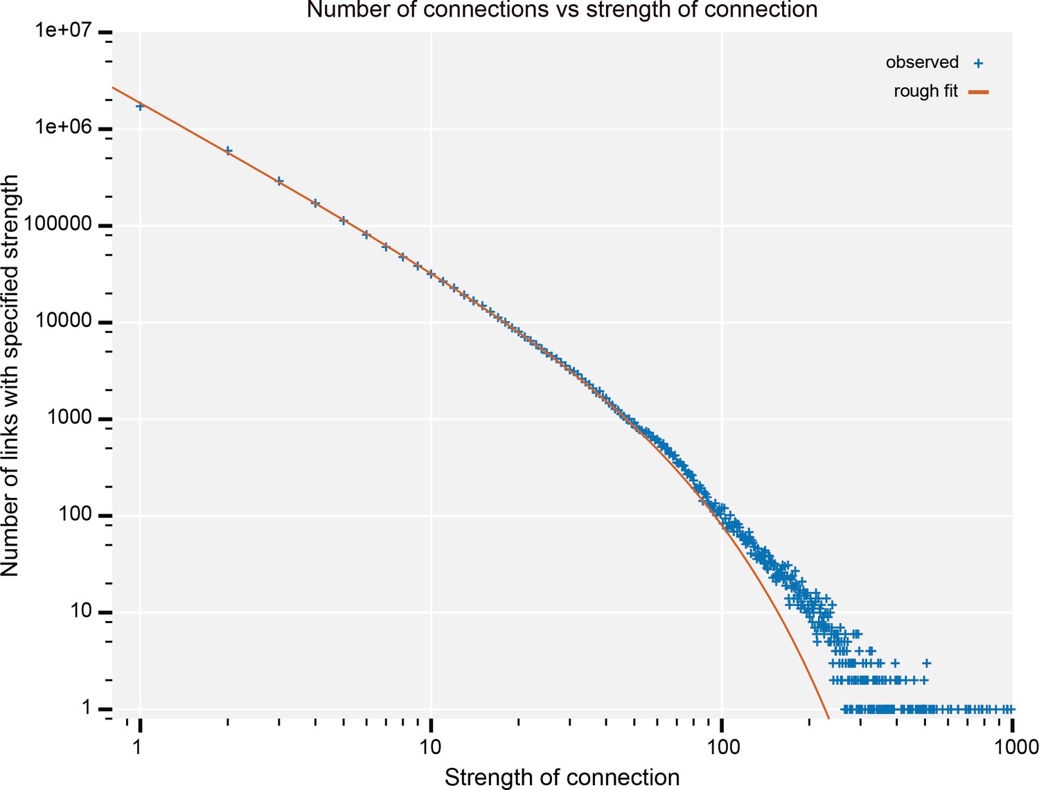
The number of connections with a given strength.
Up to a strength of 100, this is well described by a power law (exponent −1.67) with exponential cutoff (at N = 42). Data available in Figure 21—source data 1.
-
Figure 21—source data 1
Data for Figure 21.
The first column is a synapse count of a connection. The second column tells how many connections of that strength exist.
- https://cdn.elifesciences.org/articles/57443/elife-57443-fig21-data1-v4.txt
Figure 22
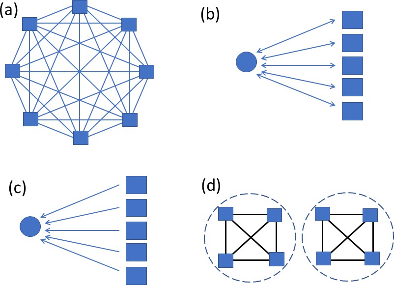
Large motifs searched for.
Squares represent abundant types with at least 20 instances. Circles represent sparse types with at most two instances. Panel (a) shows a clique, where all possible connections are present. (b) It shows bidirectional connections between a sparse type and all instances of an abundant type. (c) It shows unidirectional connections from all of an abundant type to a sparse type. Panel (d) illustrates a cell type that does not form a clique overall, but does within each of two compartments.
Figure 23
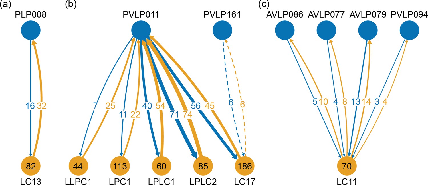
One to many motifs found in the optic circuits.
Cell types consisting of a single cell, or a left-right pair, are shown at the top of the diagram. Corresponding cell type, each with many instances, are shown at the bottom of the diagram, with the number of cells per type shown inside. The arrows show the average count of synaptic connections per one cell of the bottom group. (a) An example of the most common case is shown. Here one cell, PLP008, has bidirectional connections to all 82 cells of type LC13. (b) It shows a single cell with exhaustive connections to several types. (c) It shows an alternative motif where several cells form these one-to-many connections.
Figure 24
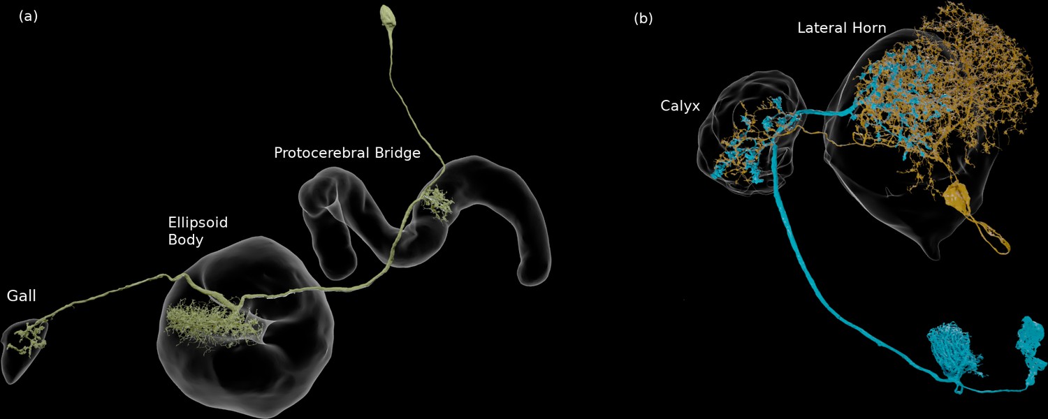
Neural connection patterns.
(a) An EPG neuron, with arbors in three compartments. (b) Two neurons that connect in more than one compartment, in this case the calyx and the lateral horn. They are each pre- and postsynaptic to each other in both compartments.
Figure 25
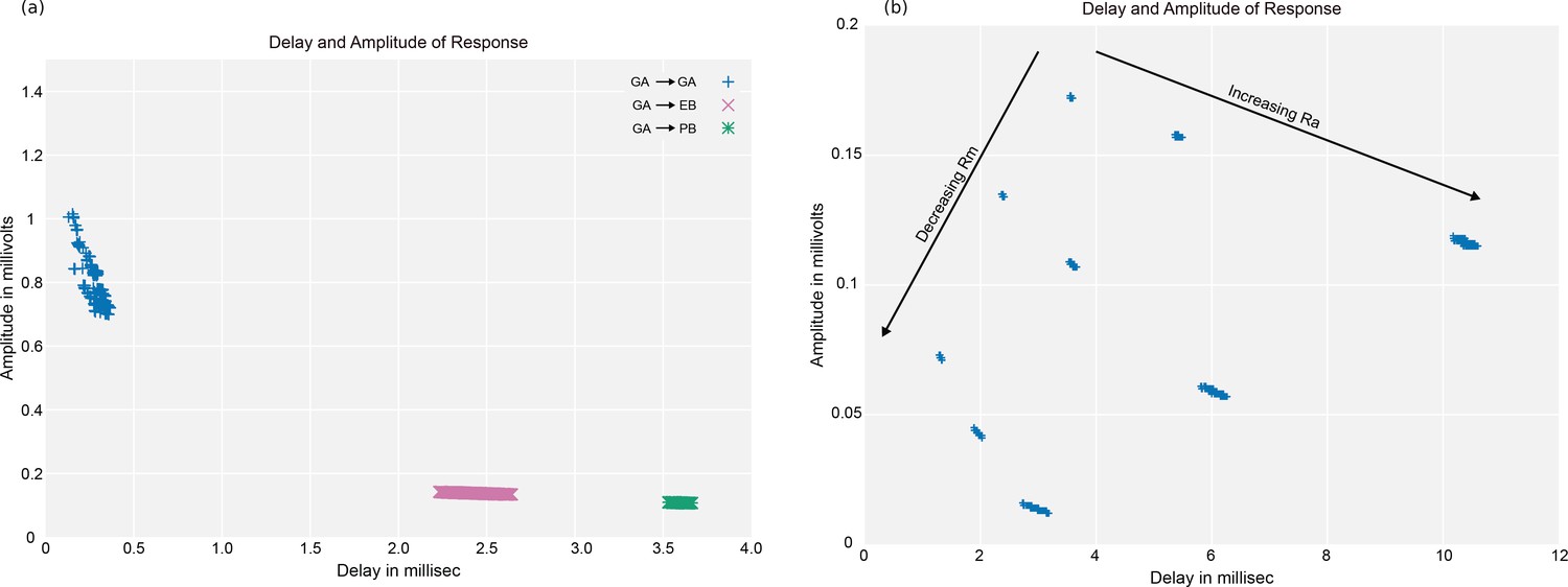
Delay versus amplitude plots for a neuron.
(a) The linear response to inputs in the gall (GA) for an EPG neuron, which also has arbors in the ellipsoid body (EB) and the protocerebral bridge (PB). Each point in the modeled plot shows the time each response reached its peak amplitude (the delay), and the amplitude at that time, for an input injected at one of the PSDs in the gall. (b) Delays and amplitudes for gall to PB response, for all combinations of three values of cytoplasmic resistance and three values of membrane resistance . Data available in Figure 25—source datas 1–4.
-
Figure 25—source data 1
Data for Figure 25A (ellipsoid body).
The first column is the delay in milli-seconds, the second the amplitude in mv, the third the connection type.
- https://cdn.elifesciences.org/articles/57443/elife-57443-fig25-data1-v4.eb.txt
-
Figure 25—source data 2
Data for Figure 25A (gall).
The first column is the delay in milli-seconds, the second the amplitude in mv, the third the connection type.
- https://cdn.elifesciences.org/articles/57443/elife-57443-fig25-data2-v4.ga.txt
-
Figure 25—source data 3
Data for Figure 25A (protocerebral bridge).
The first column is the delay in milli-seconds, the second the amplitude in mv, the third the connection type.
- https://cdn.elifesciences.org/articles/57443/elife-57443-fig25-data3-v4.pb.txt
-
Figure 25—source data 4
Data for Figure 25B.
The first column is the delay in milli-seconds, the second the amplitude in mv, the third the connection type.
- https://cdn.elifesciences.org/articles/57443/elife-57443-fig25-data4-v4.txt
Figure 26
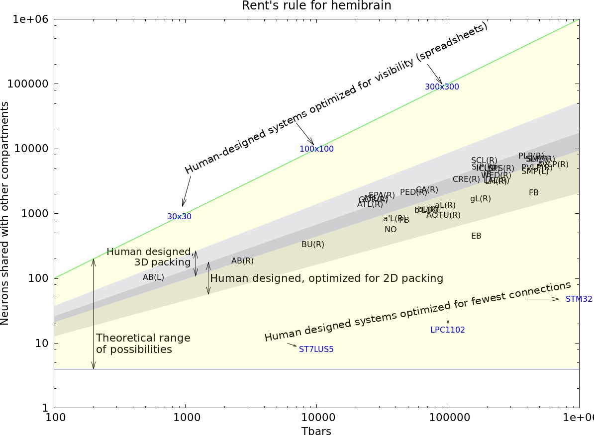
Rent’s rule for the hemibrain.
The yellow region encompasses the theoretical bounds for computation. Four varieties of human-designed systems are shown. Those designed for visibility into computation achieve the upper bound, while those designed for minimum communication approach the lower bounds (Microprocessors ST7LU55, LPC1102, and STM32). Human designed systems where efficient packing is the main criterion occupy the shaded area (in 2D and 3D). The characteristics of the primary compartments completely contained in the reconstructed volume are shown with alphanumeric labels. The hemibrain compartments fall very nearly in the same range as human designed systems designed for efficient packing. Data available in Figure 26—source data 1.
-
Figure 26—source data 1
Data for Figure 26.
The first column is the compartment name, the second the number of TBars contained, and the fifth column the number of connections.
- https://cdn.elifesciences.org/articles/57443/elife-57443-fig26-data1-v4.txt
Appendix 1—figure 1
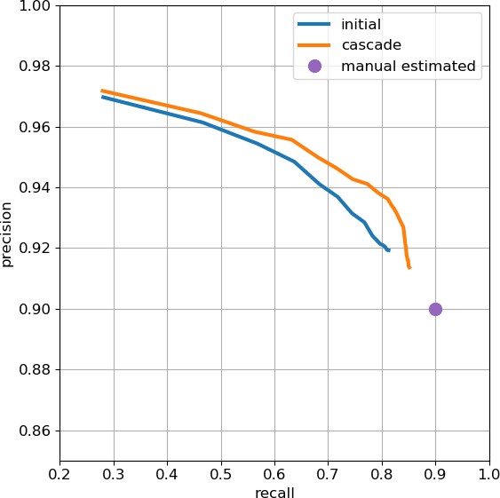
Precision-recall plot of T-bar prediction.
The purple intercept indicates estimated manual agreement rate of 0.9. Data available in Appendix 1—figure 1—source data 1.
-
Appendix 1—figure 1—source data 1
Data for Appendix 1—figure 1.
Column A: initial recall; column B: initial precision; column C: cascade recall; column D: cascade precision.
- https://cdn.elifesciences.org/articles/57443/elife-57443-app1-fig1-data1-v4.csv
Appendix 1—figure 2
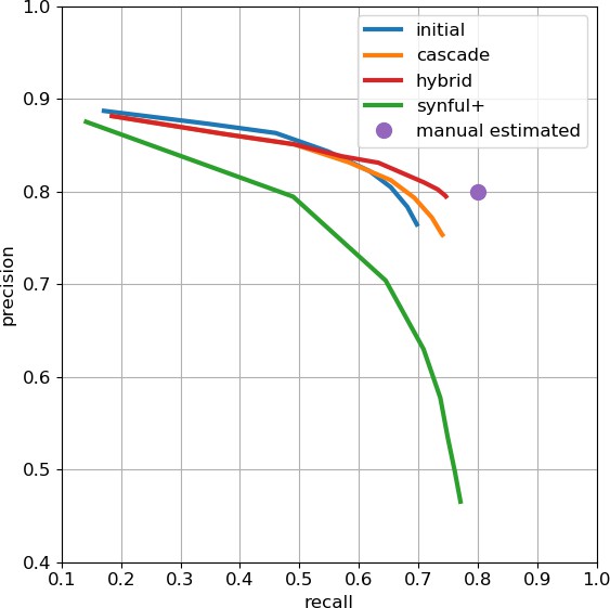
Precision-recall plot of end-to-end synapse prediction.
The purple intercept indicates estimated manual agreement rate of 0.8. Data available in Appendix 1—figure 2—source data 1.
-
Appendix 1—figure 2—source data 1
Data for Appendix 1—figure 2.
Column A: initial recall; column B: initial precision; column C: cascade recall; column D: cascade precision; column E: hybrid recall; column F: hybrid precision; column G: synfulp recall; column H: synfulp precision.
- https://cdn.elifesciences.org/articles/57443/elife-57443-app1-fig2-data1-v4.csv
Appendix 1—figure 3
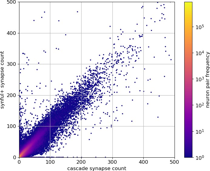
Comparison of synful+ connection strength versus cascade connection strength (truncated at a connection strength of 500 for clarity, omitting 40 edges from each prediction set).
Data available in Appendix 1—figure 3—source data 1.
-
Appendix 1—figure 3—source data 1
Data for Appendix 1—figure 3.
Column A: cascade synapse count; column B: synfulp synapse count; column C: frequency of this pair in our data.
- https://cdn.elifesciences.org/articles/57443/elife-57443-app1-fig3-data1-v4.csv
Tables
Table 1
Brain regions contained and defined in the hemibrain, following the naming conventions of Ito et al., 2014 with the addition of (R) and (L) to specify the side of the soma for that region.
Italics indicate master regions not explicitly defined in the hemibrain. Region LA is not included in the volume. The regions are hierarchical, with the more indented regions forming subsets of the less indented. The only exceptions are dACA, lACA, and vACA which are considered part of the mushroom body but are not contained in the master region MB.
| OL(R) | Optic lobe | CX | Central complex | LH(R) | Lateral horn |
| LA | lamina | FB | Fan-shaped body | ||
| ME(R) | Medula | FBl1 | Fan-shaped body layer 1 | SNP(R)/(L) | Superior neuropils |
| AME(R) | Accessory medulla | FBl2 | Fan-shaped body layer 2 | SLP(R) | Superior lateral protocerebrum |
| LO(R) | Lobula | FBl3 | Fan-shaped body layer 4 | SIP(R)/(L) | Superior intermediate protocerebrum |
| LOP(R) | Lobula plate | FBl4 | Fan-shaped body layer 4 | SMP(R)(L) | Superior medial protocerebrum |
| FBl5 | Fan-shaped body layer 5 | ||||
| MB(R)/(L) | Mushroom body | FBl6 | Fan-shaped body layer 6 | INP | Inferior neuropils |
| CA(R)/(L) | Calyx | FBl7 | Fan-shaped body layer 7 | CRE(R)/(L) | Crepine |
| dACA(R) | Dorsal accessory calyx | FBl8 | Fan-shaped body layer 8 | RUB(R)/(L) | Rubu |
| lACA(R) | Lateral accessory calyx | FBl9 | Fan-shaped body layer 9 | ROB(R) | Round body |
| vACA(R) | Ventral accessory calyx | EB | Ellipsoid body | SCL(R)/(L) | Superior clamp |
| PED(R) | Pedunculus | EBr1 | Ellipsoid body zone r1 | ICL(R)/(L) | Inferior clamp |
| a’L(R)/(L) | Alpha prime lobe | EBr2r4 | Ellipsoid body zone r2r4 | IB | Inferior bridge |
| a’1(R) | Alpha prime lobe compartment 1 | EBr3am | Ellipsoid body zone r3am | ATL(R)/(L) | Antler |
| a’2(R) | Alpha prime lobe compartment 2 | EBr3d | Ellipsoid body zone r3d | ||
| a’3(R) | Alpha prime lobe compartment 3 | EBr3pw | Ellipsoid body zone r3pw | AL(R)/(L) | Antennal lobe |
| aL(R)/(L) | Alpha lobe | EBr5 | Ellipsoid body zone r5 | ||
| a1(R) | Alpha lobe compartment 1 | EBr6 | Ellipsoid body zone r6 | VMNP | Ventromedial neuropils |
| a2(R) | Alpha lobe compartment 2 | AB(R)/(L) | Asymmetrical body | VES(R)/(L) | Vest |
| a3(R) | Alpha lobe compartment 3 | PB | Protocerebral bridge | EPA(R)/(L) | Epaulette |
| gL(R)/(L) | Gamma lobe | PB(R1) | PB glomerulus R1 | GOR(R)/(L) | Gorget |
| g1(R) | Gamma lobe compartment 1 | PB(R2) | PB glomerulus R2 | SPS(R)/(L) | Superior posterior slope |
| g2(R) | Gamma lobe compartment 2 | PB(R3) | PB glomerulus R3 | IPS(R)/(L) | Inferior posterior slope |
| g3(R) | Gamma lobe compartment 3 | PB(R4) | PB glomerulus R4 | ||
| g4(R) | Gamma lobe compartment 4 | PB(R5) | PB glomerulus R5 | PENP | Pariesophageal neuropils |
| g5(R) | Gamma lobe compartment 5 | PB(R6) | PB glomerulus R6 | SAD | Saddle |
| b’L(R)/(L) | Beta prime lobe | PB(R7) | PB glomerulus R7 | AMMC | Antennal mechanosensory and motor center |
| b’1(R) | Beta prime lobe compartment 1 | PB(R8) | PB glomerulus R8 | FLA(R) | Flange |
| b’2(R) | Beta prime lobe compartment 2 | PB(R9) | PB glomerulus R9 | CAN(R) | Cantle |
| bL(R)/(L) | Beta lobe | PB(L1) | PB glomerulus L1 | PRW | prow |
| b1(R) | Beta lobe compartment 1 | PB(L2) | PB glomerulus L2 | ||
| b2(R) | Beta lobe compartment 2 | PB(L3) | PB glomerulus L3 | GNG | Gnathal ganglia |
| PB(L4) | PB glomerulus L4 | ||||
| LX(R)/(L) | Lateral complex | PB(L5) | PB glomerulus L5 | Major Fiber bundles | |
| BU(R)/(L) | Bulb | PB(L6) | PB glomerulus L6 | AOT(R) | Anterior optic tract |
| LAL(R)/(L) | Lateral accessory lobe | PB(L7) | PB glomerulus L7 | GC | Great commissure |
| GA(R) | Gall | PB(L8) | PB glomerulus L8 | GF(R) | Giant Fiber (single neuron) |
| PB(L9) | PB glomerulus L9 | mALT(R)/(L) | Medial antennal lobe tract | ||
| VLNP(R) | Ventrolateral neuropils | NO | Noduli | POC | Posterior optic commissure |
| AOTU(R) | Anterior optic tubercle | NO1(R)/(L) | Nodulus 1 | ||
| AVLP(R) | Anterior ventrolateral protocerebrum | NO2(R)/(L) | Nodulus 2 | ||
| PVLP(R) | Posterior ventrolateral protocerebrum | NO3(R)/(L) | Nodulus 3 | ||
| PLP(R) | Posterior lateral cerebrum | ||||
| WED(R) | Wedge | ||||
Table 2
Regions with ≥50% included in the hemibrain, sorted by completion percentage.
The approximate percentage of the region included in the hemibrain volume is shown as ‘%inV’. ‘T-bars’ gives a rough estimate of the size of the region. ‘comp%’ is the fraction of the post-synaptic densities (PSDs) contained in the brain region for which both the PSD and the corresponding T-bar are in neurons marked ‘Traced’.
| Name | %inV | T-bars | comp% | Name | %inV | T-bars | comp% |
|---|---|---|---|---|---|---|---|
| PED(R) | 100% | 54805 | 85% | aL(R) | 100% | 95375 | 84% |
| b’L(R) | 100% | 67695 | 83% | bL(R) | 100% | 71112 | 83% |
| gL(R) | 100% | 176785 | 83% | a’L(R) | 100% | 39091 | 82% |
| EB | 100% | 164286 | 81% | bL(L) | 56% | 58799 | 81% |
| NO | 100% | 36722 | 79% | b’L(L) | 88% | 57802 | 78% |
| gL(L) | 55% | 133256 | 76% | CA(R) | 100% | 69517 | 73% |
| AB(R) | 100% | 2734 | 65% | aL(L) | 51% | 44803 | 62% |
| FB | 100% | 451031 | 62% | AL(R) | 83% | 501004 | 59% |
| AB(L) | 100% | 572 | 57% | PB | 100% | 46557 | 55% |
| AME(R) | 100% | 6045 | 51% | BU(R) | 100% | 9385 | 46% |
| CRE(R) | 100% | 137946 | 40% | AOTU(R) | 100% | 92578 | 38% |
| LAL(R) | 100% | 234388 | 38% | SMP(R) | 100% | 510937 | 34% |
| PVLP(R) | 100% | 475219 | 30% | ATL(R) | 100% | 25472 | 29% |
| SPS(R) | 100% | 253818 | 29% | ATL(L) | 100% | 28153 | 29% |
| VES(R) | 84% | 157168 | 29% | IB | 100% | 200447 | 28% |
| CRE(L) | 90% | 132656 | 28% | SIP(R) | 100% | 187493 | 26% |
| BU(L) | 52% | 7014 | 26% | GOR(R) | 100% | 27140 | 26% |
| WED(R) | 100% | 232898 | 25% | SMP(L) | 100% | 460784 | 26% |
| EPA(R) | 100% | 31438 | 26% | PLP(R) | 100% | 429949 | 26% |
| AVLP(R) | 100% | 630538 | 23% | ICL(R) | 100% | 202549 | 23% |
| SLP(R) | 100% | 487795 | 23% | LO(R) | 64% | 855251 | 22% |
| SCL(R) | 100% | 189569 | 22% | GOR(L) | 60% | 19558 | 21% |
| LH(R) | 100% | 231662 | 19% | CAN(R) | 68% | 6512 | 16% |
Table 3
Summary of the numbers and types of the neurons in the hemibrain EM dataset.
m-types is the number of morphology types; c-types the number of connectivity types; and c/t the average number of cells per connectivity type. Brain regions with repetitive array architecture tend to have higher average numbers of cells per type (see Figure 12). The cell number includes ≈4000 neurons on the contralateral side, and the percentage of contralateral cells varies between 0 and ≈50% depending on the category. For example, the central complex includes neurons on both sides of the brain, the mushroom body neurons are identified mostly on the right side, and many left-side antennal lobe sensory neurons are included as they tend to terminate bilaterally. Because of these differences, the figures shown above do not indicate the number of cells (or cell number per type) per brain side.
| Brain regions (neuropils) or neuron types | Cells | m-types | c-types | C/t | Notes |
|---|---|---|---|---|---|
| Central complex neuropil neurons | 2826 | 224 | 262 | 10.8 | |
| Mushroom body neuropil neurons | 2315 | 72 | 80 | 28.9 | Including MB-associated DANs |
| Mushroom body neuropil neurons | 2003 | 51 | 51 | 39.3 | Excluding MB-associated DANs |
| Dopaminergic neurons (DANs) | 335 | 35 | 43 | 7.8 | Including MB-associated DANs |
| Dopaminergic neurons (DANs) | 23 | 14 | 14 | 1.7 | Excluding MB-associated DANs |
| Octopaminergic neurons | 19 | 10 | 10 | 1.9 | |
| Serotonergic (5HT) neurons | 9 | 5 | 5 | 1.8 | |
| Peptidergic and secretory neurons | 51 | 12 | 14 | 3.6 | |
| Circadian clock neurons | 27 | 7 | 7 | 3.9 | |
| Fruitless gene expressing neurons | 84 | 29 | 30 | 2.8 | |
| Visual projection neurons and lobula intrinsic neurons | 3723 | 160 | 160 | 23.3 | |
| Descending neurons | 103 | 51 | 51 | 2.0 | |
| Sensory associated neurons | 2768 | 67 | 67 | 41.3 | |
| Antennal lobe neuropil neurons | 604 | 284 | 294 | 2.1 | |
| Lateral horn neuropil neurons | 1496 | 517 | 683 | 2.2 | |
| Anterior optic tubercle neuropil neurons | 243 | 77 | 80 | 3.0 | |
| Antler neuropil neurons | 81 | 45 | 45 | 1.8 | |
| Anterior ventrolateral protocerebrum neuropil neurons | 1276 | 596 | 629 | 2.0 | |
| Clamp neuropil neurons | 746 | 364 | 382 | 2.0 | |
| Crepine neuropil neurons | 333 | 108 | 115 | 2.9 | |
| Inferior bridge neuropil neurons | 264 | 119 | 119 | 2.2 | |
| Lateral accessory lobe neuropil neurons | 429 | 204 | 206 | 2.1 | |
| Posterior lateral protocerebrum neuropil neurons | 480 | 255 | 260 | 1.8 | |
| Posterior slope neuropil neurons | 621 | 303 | 311 | 2.0 | |
| Posterior ventrolateral protocerebrum neuropil neurons | 348 | 151 | 156 | 2.2 | |
| Saddle neuropil and antennal mechanosensory and motor center neurons | 219 | 96 | 99 | 2.2 | |
| Superior lateral protocerebrum neuropil neurons | 1096 | 468 | 494 | 2.2 | |
| Superior intermediate protocerebrum neuropil neurons | 220 | 90 | 92 | 2.4 | |
| Superior medial protocerebrum neuropil neurons | 1494 | 605 | 629 | 2.4 | |
| Vest neuropil neurons | 137 | 84 | 85 | 1.6 | |
| Wedge neuropil neurons | 559 | 212 | 230 | 2.4 | |
| Total | 22,594 | 5229 | 5609 | 4.0 |
Table 4
Regions with minimum or maximum characteristics, picked from those regions lying wholly within the reconstructed volume and containing at least 100 neurons.
Yellow indicates a minimum value; blue a maximal value. Volume is in cubic microns. N is the number of neurons in the region, L the number of connections between those neurons, the average number of partners (in the region), D the network diameter (the maximum length of the shortest path between neurons), the average connection strength, broken up into non-reciprocal and reciprocal. fracR is the fraction of connections that are reciprocal, and AvgDist the average number of hops (one hop corresponding to a direct synaptic connection) between any two neurons in the compartment.
| Name | Volume | N | L | D | fracR | AvgDist | ||||
|---|---|---|---|---|---|---|---|---|---|---|
| MB(R) | 309371 | 3514 | 574732 | 163.555 | 8 | 3.275 | 3.081 | 3.388 | 0.632 | 2.215 |
| bL(R) | 29695 | 1171 | 108250 | 92.442 | 8 | 2.019 | 1.856 | 2.122 | 0.613 | 2.090 |
| EB | 93932 | 555 | 58789 | 105.926 | 5 | 10.087 | 4.610 | 12.215 | 0.720 | 1.798 |
| AB(L) | 526 | 100 | 1250 | 12.500 | 4 | 2.182 | 1.765 | 2.687 | 0.453 | 1.938 |
| PLP(R) | 367711 | 6913 | 244182 | 35.322 | 15 | 2.791 | 2.479 | 3.866 | 0.225 | 3.148 |
| SNP(R) | 1076257 | 9130 | 811279 | 88.859 | 13 | 3.026 | 2.552 | 4.539 | 0.239 | 2.724 |
| RUB(L) | 834 | 128 | 623 | 4.867 | 6 | 7.313 | 2.766 | 20.253 | 0.260 | 2.727 |
| EPA(R) | 29947 | 1483 | 18848 | 12.709 | 13 | 2.224 | 2.152 | 2.700 | 0.131 | 3.471 |
Table 5
Cell types that form cliques and near-cliques in the hemibrain data.
To be included, a cell type must have at least 20 cell instances, 90% or more of which have bidirectional connections to at least 90% of cells of the same type. Coverage is the fraction of all possible edges in the clique that are present with any synapse count >0. Average strength is the average number of synapses in each connection. Synapses is the total number of synapses in the clique.
| Type | Region | Cells | Coverage | Avg. strength | Synapses |
|---|---|---|---|---|---|
| KCab-p | MB | 59/60 | 3455/3540 | 5.13 | 17722 |
| Delta7 | PB, CX | 42/42 | 1719/1722 | 14.21 | 24433 |
| ER2_c | EB, CX | 21/21 | 420/420 | 33.76 | 14180 |
| ER3w | EB, CX | 20/20 | 380/380 | 28.00 | 10639 |
| ER4d | EB, CX | 25/25 | 600/600 | 54.94 | 32961 |
| ER5 | EB, CX | 20/20 | 380/380 | 26.61 | 10111 |
| PFNa | NO(R) | 29/29 | 811/812 | 6.74 | 5467 |
| PFNa | NO(L) | 29/29 | 811/812 | 7.22 | 5858 |
| PFNd | NO(R) | 20/20 | 377/380 | 7.69 | 2899 |
| PFNd | NO(L) | 20/20 | 378/380 | 7.60 | 2874 |
Table 6
Values reported in the literature.
| Reference | , F/m2 | ||
|---|---|---|---|
| Borst (Borst and Haag, 1996), CH cells | 0.60 | 0.25 | 0.015 |
| Borst (Borst and Haag, 1996), HS cells | 0.40 | 0.20 | 0.009 |
| Borst (Borst and Haag, 1996), VS cells | 0.40 | 0.20 | 0.008 |
| Gouwens (Gouwens and Wilson, 2009), DM1 cell 1 | 1.62 | 0.83 | 0.026 |
| Gouwens (Gouwens and Wilson, 2009), DM1 cell 2 | 1.02 | 2.04 | 0.015 |
| Gouwens (Gouwens and Wilson, 2009), DM1 cell 3 | 2.66 | 2.08 | 0.008 |
| Gouwens (Gouwens and Wilson, 2009), dendrite 1 | 2.44 | 1.92 | 0.008 |
| Gouwens (Gouwens and Wilson, 2009), dendrite 2 | 2.66 | 2.08 | 0.008 |
| Gouwens (Gouwens and Wilson, 2009), dendrite 3 | 3.11 | 2.64 | 0.006 |
| Cuntz (Cuntz et al., 2013), HS cells | 4.00 | 0.82 | 0.006 |
| Meier (Meier and Borst, 2019), CT1 cells | 4.00 | 0.80 | 0.006 |
Appendix 1—table 1
FIB-SEM imaging conditions.
| Sample ID | Electron beam energy (kV) | Sample bias (kV) | Landing energy (kV) | SEM current (nA) | SEM scan rate (MHz) | x-y pixel (nm) | z-step (nm) |
|---|---|---|---|---|---|---|---|
| Z0115-22_Sec22 | 1.2 | 0 | 1.2 | 4 | 4 | 8 | 2 |
| Z0115-22_Sec23 | 1.2 | 0 | 1.2 | 4 | 4 | 8 | 2 |
| Z0115-22_Sec24 | 0.6 | 0.6 | 1.2 | 4 | 2 | 8 | 2 |
| Z0115-22_Sec25 | 0.6 | 0.6 | 1.2 | 4 | 2 | 8 | 2 |
| Z0115-22_Sec26 | 0.6 | 0.6 | 1.2 | 4 | 2 | 8 | 2 |
| Z0115-22_Sec27 | 0.6 | 0.6 | 1.2 | 4 | 2 | 8 | 2 |
| Z0115-22_Sec28 | 1.2 | 0 | 1.2 | 4 | 4 | 8 | 2 |
| Z0115-22_Sec29 | 1.2 | 0 | 1.2 | 4 | 4 | 8 | 2 |
| Z0115-22_Sec30 | 1.2 | 0 | 1.2 | 4 | 4 | 8 | 2 |
| Z0115-22_Sec31 | 1.2 | 0 | 1.2 | 4 | 4 | 8 | 4 |
| Z0115-22_Sec32 | 1.2 | 0 | 1.2 | 4 | 4 | 8 | 4 |
| Z0115-22_Sec33 | 1.2 | 0 | 1.2 | 4 | 4 | 8 | 4 |
| Z0115-22_Sec34 | 1.2 | 0 | 1.2 | 4 | 4 | 8 | 4 |
Appendix 1—table 2
Bounding boxes within the hemibrain volume used for training CycleGAN models.
Coordinates and sizes are given for [32 nm]3 voxels. The same physical area of the hemibrain volume was used to train both 32 nm and 16 nm CycleGAN models.
| Tab | Start | Size | ||||
|---|---|---|---|---|---|---|
| X | Y | Z | X | Y | Z | |
| reference | 4633 | 3792 | 2000 | 1374 | 2000 | 2000 |
| 22 | 8089 | 4030 | 1744 | 518 | 2000 | 2000 |
| 23 | 7435 | 3925 | 2101 | 654 | 2000 | 2000 |
| 24 | 6713 | 2939 | 4094 | 722 | 2000 | 2000 |
| 25 | 6017 | 2895 | 3635 | 694 | 2000 | 2000 |
| 28 | 3980 | 4944 | 3495 | 638 | 2000 | 2000 |
| 29 | 3307 | 2414 | 4094 | 666 | 2000 | 2000 |
| 30 | 2649 | 2519 | 4094 | 657 | 2000 | 2000 |
| 31 | 1979 | 2750 | 4094 | 670 | 2000 | 2000 |
| 32 | 1312 | 3065 | 4094 | 667 | 2000 | 2000 |
| 33 | 668 | 3101 | 3520 | 663 | 2000 | 2000 |
| 34 | 1 | 3112 | 3520 | 660 | 2000 | 2000 |
Appendix 1—table 3
ROIs within the hemibrain volume used for CycleGAN checkpoint selection.
| Tab | Voxel Res. [nm] | Start | Size | ||||
|---|---|---|---|---|---|---|---|
| X | Y | Z | X | Y | Z | ||
| 22 | 32 | 8092 | 4392 | 5447 | 500 | 936 | 936 |
| 23 | 32 | 7435 | 2479 | 4979 | 500 | 936 | 936 |
| 24 | 32 | 6717 | 5414 | 4873 | 500 | 936 | 936 |
| 25 | 32 | 6010 | 3960 | 6235 | 500 | 936 | 936 |
| 28 | 32 | 3971 | 2591 | 2954 | 500 | 936 | 936 |
| 29 | 32 | 3471 | 4252 | 2224 | 500 | 936 | 936 |
| 30 | 32 | 2650 | 2995 | 4875 | 500 | 936 | 936 |
| 31 | 32 | 1982 | 3196 | 4875 | 500 | 936 | 936 |
| 32 | 32 | 1311 | 3141 | 4873 | 500 | 936 | 936 |
| 33 | 32 | 664 | 2850 | 4875 | 500 | 936 | 936 |
| 34 | 32 | 0 | 1900 | 4500 | 500 | 5000 | 2500 |
| 22 | 16 | 16080 | 8353 | 9871 | 1034 | 936 | 936 |
| 25 | 16 | 11900 | 12657 | 12636 | 1406 | 936 | 936 |
| 25 | 16 | 11900 | 5266 | 10578 | 1408 | 936 | 936 |
| 28 | 16 | 7900 | 9279 | 4613 | 1297 | 936 | 936 |
| 29 | 16 | 6550 | 8520 | 4613 | 1333 | 936 | 936 |
| 30 | 16 | 5250 | 7997 | 7510 | 1315 | 936 | 936 |
| 31 | 16 | 3860 | 7749 | 7510 | 1340 | 936 | 936 |
| 32 | 16 | 2550 | 9482 | 4225 | 1334 | 936 | 936 |
| 33 | 16 | 1280 | 7176 | 12265 | 1298 | 936 | 936 |
| 34 | 16 | 0 | 7587 | 12265 | 1328 | 936 | 936 |
Appendix 1—table 4
Criteria for agglomerating priority groups.
If an agglomeration decision fulfills the criteria for multiple priority groups, it is assigned to the one with the lowest resulting score.
| Group | Segmentation | Criterion | Score |
|---|---|---|---|
| 1 | S32 | ||
| 2 | S16 | A and B are classified as neuropil | |
| 3 | S16 | ||
| 4 | S16 | A and B are classified as neuropil | |
| 5 | S16 | ||
| 6 | S32 | A and B are classified as neuropil | |
| 7 | S16 | ||
| 8 | S16 | A and B are classified as neuropil | |
| 9 | S16 | ||
| 10 | S8 | None | |
| 11 | S32 | None | |
| 12 | S16 | None |
Appendix 1—table 5
Corresponding short and anatomical names for cell types in the central complex.
These types were determined by different methods and different researchers, using different criteria.
| Short | Long | Short | Long | Short | Long | Short | Long | |||
|---|---|---|---|---|---|---|---|---|---|---|
| vDeltaA_a | AF | FB3B | EBCREFB3 | FB6C_a | SIPSMPFB6_1 | FC2B | FB1d,3,5,6CRE | |||
| vDeltaA_b | FB1D0FB8 | FB3C | LALSMPFB3 | FB6C_b | SIPSMPFB6_1 | FC2C | FB1d,3,6,7CRE | |||
| vDeltaB | FB1D0FB7_1 | FB3D | LALCREFB3 | FB6D | SMPFB6 | FC3 | FB2,3,5,6CRE | |||
| vDeltaC | FB1D0FB7_2 | FB3E | SMPLALFB3 | FB6E | SIPSMPFB6_2 | FR1 | FB2-5RUB | |||
| vDeltaD | FB1D0FB6 | FB4A | CRESMPFB4_1 | FB6F | SMPSIPFB6_3 | FR2 | FB2-4RUB | |||
| vDeltaE | FB1,2,3D0FB6v | FB4B | NO2LALFB4 | FB6G | SIPSMPFB6_3 | FS1A | FB2-6SMPSMP | |||
| vDeltaF | FB1,2,3D0FB5d | FB4C | CRENO2FB4_1 | FB6H | SMPSIPFB6_4 | FS1B | FB2,5,SMPSMP | |||
| vDeltaG | FB1,2D0FB5d | FB4D | CRESMPFB4_2 | FB6I | SMPSIPFB6_5 | FS2 | FB3,6SMP | |||
| vDeltaH | FB1,2D0FB5 | FB4E | CRELALFB4_1 | FB6J | FB6_1 | FS3 | FB1d,3,6,7SMP | |||
| vDeltaI | FB1D0FB5 | FB4F_a | CRELALFB4_2 | FB6K | SMPSIPFB6_6 | FS4A | FB3,8ABSMP | |||
| vDeltaJ | FB1D0FB5v | FB4F_b | CRELALFB4_2 | FB6L | FB6_2 | FB1,3,8SMP | ||||
| vDeltaK | FB1vD0FB4d5v | FB4G | CRELALFB4_3 | FB6M | WEDLALFB6 | FS4B | FB2,8ABSMP | |||
| vDeltaL | FB1vD0FB4 | FB4H | CRELALFB4_4 | FB6N | CRESMPFB6_1 | FB1,2,8SMP | ||||
| vDeltaM | FB1vD0FB4 | FB4I | LALCREFB4 | FB6O | SIPSMPFB6_4 | FS4C | FB2,6,7SMP | |||
| hDeltaA | FB4D5FB4 | FB4J | CRELALFB4_5 | FB6P | SMPCREFB6_1 | GLNO | LGNO | |||
| hDeltaB | FB3,4vD5FB3,4v | FB4K | CRESMPFB4_3 | FB6Q | SIPSMPFB6_5 | IbSpsP | IbSpsP | |||
| hDeltaC | FB2,6D7FB6 | FB4L | LALSIPFB4 | FB6R | SMPSIPFB6_7 | LCNOp | LCNp | |||
| hDeltaD | FB1,8D3FB8 | FB4M | CRENO2FB4_2 | FB6S | SIPSMPFB6_6 | LCNOpm | LCNpm | |||
| hDeltaE | FB1,7D3FB7 | FB4N | SMPCREFB4 | FB6T | SIPSMPFB6_7 | LNO1 | LNO1 | |||
| hDeltaF | FB1,6d,7D2FB6,7 | FB4O | CRESMPFB4d | FB6U | SMPCREFB6_2 | LNO2 | LNO2 | |||
| hDeltaG | FB2,3,5d6vD3FB6v | FB4P_a | CRESMPFB4_ 4 | FB6V | SMPCREFB6_3 | LNO3 | LNO3 | |||
| hDeltaH | FB2d,4D3FB5 | FB4P_b | CRESMPFB4_ 4 | FB6W | CRESMPFB6_2 | LNOa | LNa | |||
| hDeltaI | FB2,3,4,5D5FB4,5v | FB4Q_a | CRESMPFB4_5 | FB6X | SMPCREFB6_4 | LPsP | LPsP | |||
| hDeltaJ | FB1,2,3,4D5FB4,5 | FB4Q_b | CRESMPFB4_5 | FB6Y | SMPSIPFB6_8 | Delta7 | Delta7 | |||
| hDeltaK | EBFB3,4D5FB6 | FB4R | CREFB4 | FB6Z | SMPSIPFB6_9 | EL | EBGAs | |||
| hDeltaL | FB2,6D5FB6d | FB4X | CRESIPFB4,5 | FB7A | SIPSLPFB7 | EPG | EPG | |||
| hDeltaM | FB2,4D3FB5 | FB4Y | EBCREFB4,5 | FB7B | SMPSLPFB7 | EPGt | EPGt | |||
| FB1A | SMPSIPFB1,3 | FB4Z | FB4d5v | FB7C | SMPSIPFB7_1 | P1-9 | PBPB | |||
| FB1B | SMPSLPFB1d | FB5A | LALCREFB5 | FB7D | FB7,6 | P6-8P9 | P6-8P9 | |||
| FB1C | LALNOmFB1 | FB5AA | SMPCREFB5_10 | FB7E | SMPSIPFB7_2 | PEG | PEG | |||
| FB1D | SLPFB1d | FB5AB | SIPCREFB5d | FB7F | SMPSIPFB7_3 | PEN_a(PEN1) | PEN1 | |||
| FB1E_a | SIPSMPFB1d | FB5B | SMPSIPFB5d_1 | FB7G | SMPFB7,8 | PEN_b(PEN2) | PEN2 | |||
| FB1E_b | SLPSIPFB1d | FB5C | SMPCREFB5_1 | FB7H | SMPFB7 | PFGs | PFGs | |||
| FB1F | SMPSIPFB1d | FB5D | CRESMPFB5_1 | FB7I | SMPSIPFB7,6 | PFL1 | PFLC | |||
| FB1G | SMPSIPFB1d,3 | FB5E | CRESMPFB5_2 | FB7J | FB7,8 | PFL2 | PB1-4FB1,2,4,5LAL | |||
| FB1H | CRENO2,3FB1-4 | FB5F | SMPCREFB5_2 | FB7K | SLPSIPFB7 | PFL3 | PB1-7FB1,2,4,5LAL | |||
| FB1I | SMPSIPFB1d,7 | FB5G | SMPSIPFB5,6 | FB7L | SMPSIPFB7_4 | PFNa | PFNa | |||
| FB1J | SLPSIPFB1,7,8 | FB5H | CRESMPFB5_3 | FB7M | SMPSIPFB7_5 | PFNd | PFNd | |||
| FB2A | NOaLALFB2 | FB5I | SMPCREFB5_3 | FB8A | SLPSMPFB8_1 | PFNm_a | PFNm_a | |||
| FB2B_a | LALCREFB2_1 | FB5J | SMPFB5 | FB8B | PLPSLPFB8 | PFNm_b | PFNm_b | |||
| FB2B_b | LALCREFB2_1 | FB5K | CREFB5 | FB8C | SMPFB8 | PFNp_a | PFNp_a | |||
| FB2C | SMPCREFB2_1 | FB5L | CRESMPFB5_4 | FB8D | SLPSMPFB8_2 | PFNp_b | PFNp_b | |||
| FB2D | LALCREFB2_2 | FB5M | CRESMPFB5_5 | FB8E | SMPSIPFB8_1 | PFNp_c | PFNp_c | |||
| FB2E | SCLSMPFB2 | FB5N | SMPCREFB5_4 | FB8F_a | SIPSLPFB8 | PFNp_d | PFNp_d | |||
| FB2F_a | SIPSMPFB2 | FB5O | SMPCREFB5_5 | FB8F_b | SIPSLPFB8 | PFNp_e | PFNp_e | |||
| FB2F_b | SIPSMPFB2 | FB5P | SMPCREFB5_6 | FB8G | SMPSIPFB8_2 | PFNv | PFNv | |||
| FB2F_c | SIPSMPFB2 | FB5Q | SMPCREFB5d | FB8H | SMPSLPFB8 | PFR_a | PFR_a | |||
| FB2G_a | SMPSIPFB2 | FB5R | FB5 | FB8I | SMPSIPFB8_3 | PFR_b | PFR_b | |||
| FB2G_b | SIPLALFB2 | FB5S | FB5d,6v | FB9A | SLPFB9_1 | SA1_a | SlpA | |||
| FB2H_a | SIPSCLFB2 | FB5T | CRESMPFB5_6 | FB9B_a | SLPFB9_2 | SA1_b | SlpA | |||
| FB2H_b | SIPSCLFB2 | FB5U | FB5d | FB9B_b | SLPFB9_2 | SA1_c | SlpA | |||
| FB2I_a | SMPATLFB2 | FB5V | CRELALFB5 | FB9B_c | SLPFB9_2 | SA2_a | SlpA | |||
| FB2I_b | SMPATLFB2 | FB5W | SMPCREFB5_7 | FB9B_d | SLPFB9_2 | SA2_b | SlpA | |||
| FB2J | SMPPLPFB2 | FB5X | SMPCREFB5_8 | FB9B_e | SLPFB9_2 | SA3 | SlpA | |||
| FB2K | LALSMPFB2 | FB5Y | SMPSIPFB5d_2 | FB9C_a | SLPFB9_2 | SAF | SlpAF | |||
| FB2L | SMPCREFB2_2 | FB5Z | SMPCREFB5_9 | FB9C_b | SLPFB9_2 | SpsP | SpsP | |||
| FB2M | SIPCREFB2 | FB6A | SMPSIPFB6_1 | FC1 | FB2CRE | |||||
| FB3A | LALNO2FB3 | FB6B | SMPSIPFB6_2 | FC2A | FB1-5CRE |
Appendix 1—table 6
Naming scheme for neurons.
The neuron types that are known to exist but are not yet identified conclusively in the hemibrain data are not shown in the list.
| Connectivity types |
|---|
| _a, _b, _c, _d, etc. at the end of the morphology type names shown below |
| Morphology types |
| Central complex neuropil neurons |
| Delta7 (protocerebral bridge Delta seven between glomeruli) |
| vDeltaA-M (fan-shaped body vertical Delta within a single column [type ID]) |
| hDeltaA-M (fan-shaped body horizontal Delta across columns [type ID]) |
| EL (Ellipsoid body - Lateral accessory lobe) |
| EPG (Ellipsoid body - Protocerebral bridge - Gall) |
| EPGt (Ellipsoid body - Protocerebral bridge - Gall tip) |
| ER1-6 (Ellipsoid body Ring neuron [type ID]) |
| ExR1-8 (Extrinsic Ring neuron [type ID]) |
| FB1A-9C (Fan-shaped Body [layer ID][type ID]) |
| FC1A-3 (Fan-shaped body - Crepine [type ID]) |
| FR1, 2 (Fan-shaped body - Rubus [type ID]) |
| FS1A-4C (Fan-shaped body - Superior medial protocerebrum [type ID]) |
| IbSpsP (Inferior bridge - Superior posterior slope - Protocerebral bridge) |
| LCNOp, pm (Lateral accessory lobe - Crepine - NOduli [compartment ID]) |
| LNOa (Lateral accessory lobe - NOduli [compartment ID]) |
| LNO1-3 (Lateral accessory lobe - NOduli [type ID]) |
| GLNO (Gall - Lateral accessory lobe - Noduli) |
| LPsP (Lateral accessory lobe - Posterior slope - Protocerebral bridge) |
| P1-9 (Protocerebral bridge [glomerulus ID]) |
| P6-8P9 (Protocerebral bridge [glomerulus ID1] Protocerebral bridge [glomerulus ID2]) |
| PEG (Protocerebral bridge - Ellipsoid body - Gall) |
| PEN_a(PEN1), _b(PEN2) (Protocerebral bridge - Ellipsoid body - Noduli [subtype ID]) |
| PFGs (Protocerebral bridge - Fan-shaped body - Gall surrounding region) |
| PFL1-3 (Protocerebral bridge - Fan-shaped body - Lateral accessory lobe [type ID]) |
| PFNa, d, m, p, v (Protocerebral bridge - Fan-shaped body - Noduli [compartment ID]) |
| PFR (Protocerebral bridge - Fan-shaped body - Round body) |
| SA1-3 (Superior medial protocerebrum - Asymmetrical body [type ID]) |
| SAF (Superior medial protocerebrum - Asymmetrical body - Fan-shaped body) |
| SpsP (Superior posterior slope - Protocerebral bridge) |
| Mushroom body neuropil neurons |
| KCab-c, m, p, s (Kenyon Cell alpha-beta lobe - [layer ID]) |
| KCa’b’-ap1, ap2, m (Kenyon Cell alpha’-beta’ lobe - [layer ID]) |
| KCg-d, m, s, t (Kenyon Cell gamma lobe - [layer ID]) |
| MBON01-35 (Mushroom Body Output Neuron [type ID]) |
| APL (Anterior Paired Lateral) |
| DPM (Dorsal Paired Medial) |
| MB-C1 (Mushroom Body - Calyx [type ID]) |
| PAM01-15 (MB-associated DAN, Protocerebral Anterior Medial cluster [type ID]) |
| PPL101-106 (MB-associated DAN, Protocerebral Posterior Lateral 1 cluster [type ID]) |
| Dopaminergic neurons (DANs) |
| PPL107, 08 (Protocerebral Posterior Lateral 1 cluster [type ID]) |
| PPL201-04 (Protocerebral Posterior Lateral 2 cluster [type ID]) |
| PPM1201-05 (Protocerebral Posterior Medial 1/2 clusters [type ID]) |
| PAL01-03 (Protocerebral/paired Anterior Lateral cluster [type ID]) |
| Octopaminergic neurons |
| OA-ASM1-3 (OctopAmine - Anterior Superior Medial [type ID]) |
| OA-VPM3, 4 (OctopAmine - ventral paired median [type ID]) |
| OA-VUMa1-7 (OctopAmine - ventral unpaired median anterior [type ID]) |
| Serotonergic (5HT) neurons |
| 5-HTPLP01 (5-HT Posterior lateral protocerebrum [type ID]) |
| 5-HTPMPD01 (Posterior medial protocerebrum, dorsal [type ID]) |
| 5-HTPMPV01, 03 (Posterior medial protocerebrum, ventral [type ID]) |
| CSD (Serotonin-immunoreactive Deutocerebral neuron) |
| Peptidergic and secretory neurons |
| AstA1 (Allatostatin A) |
| CRZ01, 02 (Corazonin [type ID]) |
| DSKMP1A, 1B, 3 (Drosulfakinin medial protocerebrum [type ID]) |
| NPFL1-I (Neuropeptide F lateral large) |
| NPFP1 (Neuropeptide F dorso median) |
| PI1-3 (Pars Intercerebralis [type ID] Insulin Producing Cell candidates) |
| SIFa (SIFamide) |
| Circadian clock neurons |
| DN1a (Dorsal Neuron 1 anterior) |
| DN1pA, B (Dorsal Neuron 1 posterior [type ID]) |
| l-LNv (large Lateral Neuron ventral) |
| LNd (Lateral Neuron dorsal) |
| LPN (Lateral Posterior Neuron) |
| s-LNv (small Lateral Neuron ventral) |
| Fruitless gene expressing neurons |
| aDT4 (anterior DeuTocerebrum [type ID]) |
| aIPg1-4 (anterior Inferior Protocerebrum [type ID]) |
| aSP-f1-4, g1-3B (anterior Superior Protocerebrum [type ID]) |
| aSP8, 10A-10C (anterior Superior Protocerebrum [type ID]) |
| pC1a-e (doublesex-expressing posterior Cells [type ID]) |
| oviDNa, b (Oviposition Descending Neuron [type ID]) |
| oviIN (Oviposition Inhibitory Neuron) |
| SAG (Sex peptide Abdominal Ganglion) |
| vpoDN (vaginal plate opening descending neuron) |
| vpoEN (vaginal plate opening excitatory neuron) |
| Visual projection neurons and intrinsic neurons of the optic lobe |
| aMe1-26 (accessory Medulla [type ID]) |
| CT1 (Complex neuropils Tangential [type ID]) |
| LC4, 6, 9–46 (Lobula Columnar [type ID]) |
| LLPC1-3 (Lobula - Lobula Plate Columnar [type ID]) |
| LPC1, 2 (Lobula Plate Columnar [type ID]) |
| LPLC1-4 (Lobula Plate - Lobula Columnar [type ID]) |
| LT1, 11, 33–47, 51–87 (Lobula Tangential [type ID]) |
| MC61-66 (Medulla Columnar [type ID]) |
| DCH (Dorsal Centrifugal Horizontal) |
| H1, 2 (Horizontal [type ID]) |
| HSN, E, S (Horizontal System North, Equatorial, South) |
| VS (Vertical System) |
| VCH (Ventral Centrifugal Horizontal) |
| Li11-20 (Lobula intrinsic [type ID]) |
| HBeyelet (Hofbauer-Buchner eyelet) |
| Descending neurons |
| DNa01-10 (Descending Neuron cell body anterior dorsal [type ID]) |
| DNb01-06 (Descending Neuron cell body anterior ventral [type ID]) |
| DNd01 (Descending Neuron outside cell cluster on the anterior surface [type ID]) |
| DNg30 (Descending Neuron cell body in the gnathal ganglion [type ID]) |
| DNp02-49 (Descending Neuron cell body on the posterior surface of the brain [type ID]) |
| DNES1-3 (Descending Neuron going out to ESophagus [type ID]) |
| Giant_Fiber descending neuron |
| MDN (Moonwalker Descending Neuron) |
| Sensory associated neurons |
| ORN_D, DA1-4, DC1-4, DL1-5, DM1-6, DP1l, m, V, VA1-7m, VC1-5, VL1-2p, VM1-7v (Olfactory Receptor Neuron_ [glomerulus ID]) |
| TRN_VP1m, 2, 3 (Thermo-Receptor Neuron_ [glomerulus ID]) |
| HRN_VP1d, 1 l, 4, 5 (Hygro-Receptor Neuron_ [glomerulus ID]) |
| JO-ABC (Johnston’s Organ auditory receptor neuron- [AMMC zone ID]) |
| OCG01-08 (OCellar Ganglion neuron [type ID]) |
| Antennal lobe neuropil neurons |
| D_adPN, DA1_lPN, DC2_adPN, DL3_lPN, DM4_vPN, DP1l_adPN, VA1d_adPN, VC2_lPN, VL2p_vPN, VM7d_adPN, VP2_l2PN, etc. (uniglomerular [glomerulus ID] _ [cell cluster ID] Projection Neuron) |
| VP1l+_lvPN, VP3+_vPN, etc. (uni+glomerular [glomerulus ID]+ _ [cell cluster ID] Projection Neuron, arborizing in a glomerulus and a few neighboring areas) |
| VP1m+VP2_lvPN1, 2, VP4+VL1_l2PN, etc. (biglomerular [glomerulus ID1]+[glomerulus ID2] _ [cell cluster ID] Projec tion Neuron, arborizing in two glomeruli) |
| M_smPNm1, 6t2, adPNm3-8, spPN4t9, 5t10, lPNm11A-13, l2PNm14-16, 3t17, 10t18, l19-22, m23, lvPNm24-48, lv2PN9t49, vPNml50-89, ilPNm90, 8t91, imPNl92 (Multiglomerular_ [cell cluster ID] Projection Neuron [antennal lobe tract ID][type ID]) |
| MZ_lvPN, lv2PN (Multiglomerular and subesophageal Zone _ [cell cluster ID] Projection Neuron) |
| Z_lvPNm1, Z_vPNml1 (subesophageal Zone only _ [cell cluster ID] Projection Neuron [antennal lobe tract ID][type ID]) |
| lLN1, 2, 7–17, v2LN2-5, 30–50, il3LN6, l2LN18-23, vLN24-29 ([cell cluster ID] Local Neuron [type ID]) |
| mAL1-6, B1-5, C1-6, D1-4 (mediodorsal Antennal Lobe neuron [type ID]) |
| AL-AST1 (Antennal Lobe - Antenno-Subesophageal Tract [type ID]) |
| AL-MBDL1 (Antennal Lobe - Median BunDLe [type ID]) |
| ALBN1 (Antennal Lobe Bilateral Neuron [type ID]) |
| ALIN1-3 (Antennal Lobe INput neuron [type ID]) |
| Lateral horn neuropil neurons |
| LHAD1a1-4a1 (Lateral Horn Anterior Dorsal cell cluster [cell cluster ID][anatomy group ID][type ID]) |
| LHAV1a1-9a1 (Lateral Horn Anterior Ventral cell cluster [cell cluster ID][anatomy group ID][type ID]) |
| LHPD1a1-5f1 (Lateral Horn Posterior Dorsal cell cluster [cell cluster ID][anatomy group ID][type ID]) |
| LHPV1c1-12a1 (Lateral Horn Posterior Ventral cell cluster [cell cluster ID][anatomy group ID][type ID]) |
| LHCENT1-14 (Lateral Horn CENTrifugal [type ID]) |
| LHMB1 (Lateral Horn - Mushroom Body [type ID]) |
| Anterior optic tubercle neuropil neurons |
| AOTU001-065 (Anterior Optic TUbercle [type ID]) |
| TuBu01-10, A, B (anterior optic Tubercle - Bulb [type ID]) |
| Antler neuropil neurons |
| ATL001-045 (Antler [type ID]) |
| Anterior ventrolateral protocerebrum neuropil neurons |
| AVLP001-596 (Anterior VentroLateral Protocerebrum [type ID]) |
| Clamp neuropil neurons |
| CL001-364 (CLamp [type ID]) |
| Crepine neuropil neurons |
| CRE001-108 (CREpine [type ID]) |
| Inferior bridge neuropil neurons |
| IB001-119 (Inferior Bridge [type ID]) |
| Lateral accessory lobe neuropil neurons |
| LAL001-204 (Lateral Accessory Lobe [type ID]) |
| Posterior lateral protocerebrum neurons |
| PLP001-255 (Posterior Lateral Protocerebrum [type ID]) |
| Posterior slope neuropil neurons |
| PS001-303 (Posterior Slope [type ID]) |
| Posterior ventrolateral protocerebrum neuropil neurons |
| PVLP001-151 (Posterior VentroLateral Protocerebrum [type ID]) |
| Saddle neuropil and antennal mechanosensory and motor center neurons |
| SAD001-095 (SADdle [type ID]) |
| AMMC-A1 (Antennal Mechanosensory and Motor Center- [type ID]) |
| Superior lateral protocerebrum neuropil neurons |
| SLP001-468 (Superior Lateral Protocerebrum [type ID]) |
| Superior intermediate protocerebrum neuropil neurons |
| SIP001-90 (Superior Intermediate Protocerebrum [type ID]) |
| Superior medial protocerebrum neuropil neurons |
| SMP001-604 (Superior Medial Protocerebrum [type ID]) |
| DGI (Dorsal Giant Interneuron) |
| Vest neuropil neurons |
| VES001-84 (VESt [type ID]) |
| Wedge neuropil neurons |
| WED001-183 (WEDge [type ID]) |
| WEDPN1-19 (WEDge Projection Neuron [type ID]) |
Additional files
-
Supplementary file 1
Spreadsheet of instances of sparse-to-many connections.
- https://cdn.elifesciences.org/articles/57443/elife-57443-supp1-v4.xlxs
-
Transparent reporting form
- https://cdn.elifesciences.org/articles/57443/elife-57443-transrepform-v4.docx
-
Appendix 1—figure 1—source data 1
Data for Appendix 1—figure 1.
Column A: initial recall; column B: initial precision; column C: cascade recall; column D: cascade precision.
- https://cdn.elifesciences.org/articles/57443/elife-57443-app1-fig1-data1-v4.csv
-
Appendix 1—figure 2—source data 1
Data for Appendix 1—figure 2.
Column A: initial recall; column B: initial precision; column C: cascade recall; column D: cascade precision; column E: hybrid recall; column F: hybrid precision; column G: synfulp recall; column H: synfulp precision.
- https://cdn.elifesciences.org/articles/57443/elife-57443-app1-fig2-data1-v4.csv
-
Appendix 1—figure 3—source data 1
Data for Appendix 1—figure 3.
Column A: cascade synapse count; column B: synfulp synapse count; column C: frequency of this pair in our data.
- https://cdn.elifesciences.org/articles/57443/elife-57443-app1-fig3-data1-v4.csv
Download links
A two-part list of links to download the article, or parts of the article, in various formats.
Downloads (link to download the article as PDF)
Open citations (links to open the citations from this article in various online reference manager services)
Cite this article (links to download the citations from this article in formats compatible with various reference manager tools)
A connectome and analysis of the adult Drosophila central brain
eLife 9:e57443.
https://doi.org/10.7554/eLife.57443


