Figures and data in Abstract rules drive adaptation in the subcortical sensory pathway

Figures
Tables
Additional files

7 figures, 2 tables and 1 additional file

Figures

Figure 1 with 1 supplement

Download asset Open asset

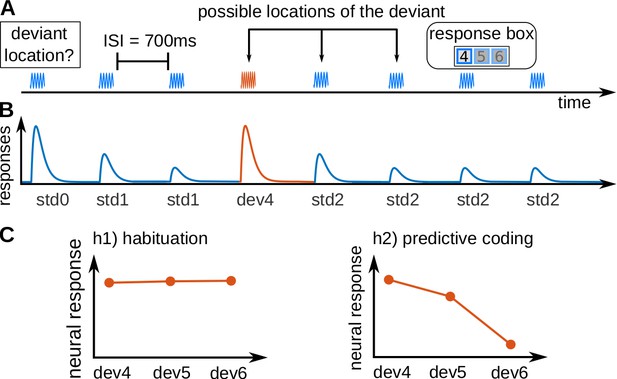
Experimental design and hypotheses.

(A) Example of a trial, consisting of a sequence of seven pure tones of a standard frequency (blue waveform) and one pure tone of a deviant frequency (fourth tone in the example; red waveform), that could be located in positions 4, 5, or 6. Subjects had to report, in each trial, the position of the deviant. Each subject completed 240 trials in total, 80 per deviant position. All tones had a duration of 50 ms and were separated by 700 ms inter-stimulus-intervals (ISIs). (B) Schematic view of the expected underlying responses in the auditory pathway for the sequence shown in A, together with the definition of the experimental variables ( $s t d 0$ : first standard; $s t d 1$ : repeated standards preceding the deviant; $s t d 2$ : standards following the deviant; $d e v x$ : deviant in position x). (C) Expected responses in the auditory pathway nuclei corresponding to the habituation (h1) and predictive coding (h2) hypotheses. Since the posterior probability of finding a deviant at locations 4, 5, or 6 after hearing 3, 4 or 5 standards is 1/3, 1/2, and 1, respectively, predictive coding predicts different BOLD responses to different deviant locations.

Figure 1—figure supplement 1

Download asset Open asset

Schematic of the GLM's design matrix of two example trials with deviants in positions 4 and 6, respectively.

Numbers in the lines for std1 and std2 indicate the parametric modulation factors.

Figure 2

Download asset Open asset

Mesoscopic stimulus-specific adaptation (SSA) in bilateral IC and MGB.

Regions within the anatomical MGB and IC ROIs showed adaptation to the repeated standards (adaptation; blue+purple) and deviant detection (red+purple). SSA (i.e. recovered responses to a deviant in voxels showing adaptation) occurred in bilateral MGB and IC (purple). Contrast patches show the voxels thresholded at $p < 0.05$ FDR-corrected for the number of voxels in each anatomical ROI.

Figure 3 with 1 supplement

Download asset Open asset

BOLD responses in the four ROIs to the three different positions of the deviants.

Kernel density estimations of the distribution of z-scores of the estimated BOLD responses, averaged over voxels of each ROI, to the three deviant positions (dev4, dev5, dev6) in each of the four ROIs: left and right IC, and left and right MGB (IC-L, IC-R, MGB-L, MGB-R). Responses to the three different standards ( $s t d 0$ , $s t d 1$ , $s t d 2$ ) are displayed for reference. Each distribution holds 19 samples, one per subject. Error bars signal the mean and standard error of the distributions. * $p < 0.05$ , ** $p < 0.005$ , *** $p < 0.0005$ , **** $p < 0.00005$ ; all p-values are Holm-Bonferroni corrected for $8 \times 4 = 32$ comparisons. $S t d 0$ , first standard; $s t d 1$ : standards preceding the deviant; $s t d 2$ : standards following the deviant; $d e v 4$ , $d e v 5$ , and $d e v 6$ : deviants at positions 4, 5, and 6, respectively.

Figure 3—figure supplement 1

Download asset Open asset

Pearson correlations between the estimated BOLD responses and predictability of the deviants at the group (A) and subject (B) level.

Violin plot shows the distribution of correlations across subjects.

Figure 4 with 1 supplement

Download asset Open asset

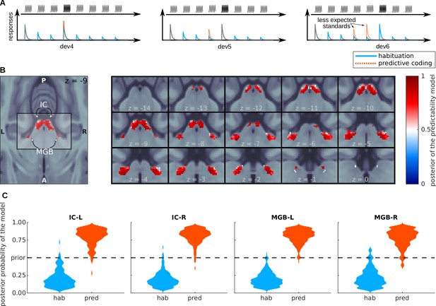
Bayesian model comparison analysis of the BOLD responses.

(A) Design of the Bayesian analysis: each model was defined according to the relative amplitudes it predicted for the different positions of the standards and deviants in the tone sequences. Note that, depending on the deviant position, standards in positions 4 and 5 were not fully expected in the predictive coding model. (B) Posterior probability map of the predictive coding model. Since we only used two models to compute the posteriors, $p < 0.5$ means that the habituation model (blue) is the most likely explanation of the data, and $p > 0.5$ means that the predictive coding model is the most likely explanation of the data. (C) Histograms showing the prevalence of each of the two models in each of the SSA regions. See also Figure 4—figure supplement 1, which shows the posterior maps and histograms for the anatomical ROIs.

Figure 4—figure supplement 1

Download asset Open asset

Posterior probability of each model across the entire anatomical ROIs.

See Figures 4 and 6 in the main text.

Figure 5

Download asset Open asset

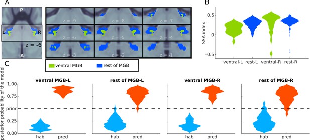
Analyses of BOLD responses in ventral MGB.

(A) Masks from Mihai et al., 2019 of the ventral MGBs (green); blue marks the remaining of the anatomical MGB ROIs. (B) The distribution of the SSA index $S I = (d e v - s t d) / (d e v + s t d)$ across each of the two subdivisions of the MGB ROIs. (C) Histograms showing the prevalence of the habituation (hab) and predictive coding (pred) models in each of the subdivisions.

Figure 6

Download asset Open asset

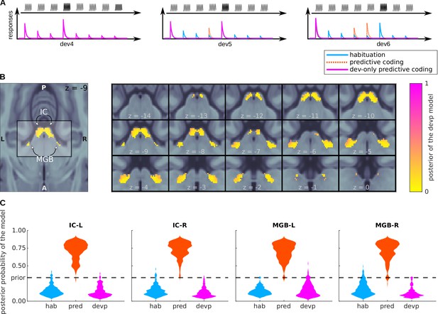
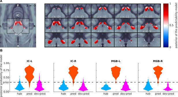
Bayesian model comparison of a variation of the predictive coding model.

(A) Design: relative amplitudes assumed by the habituation, predictive coding, and deviant-only predictive coding model. The first two models are identical to the ones defined in Figure 4A. (B) Posterior probability map of the deviant-only predictive coding model. Since three models were considered when computing the posteriors, $P < 0.33$ means that the deviant-only predictive coding model is not the most likely explanation of the data, but $P > 0.33$ does not necessarily mean that the deviant-only predictive coding model is the most likely explanation of the data. (C) Histograms showing the prevalence of each of the three models in each of the SSA regions.

Author response image 1

Download asset Open asset

Mesoscopic stimulus specific adaptation (SSA) using all deviants.

Regions within the MGB and IC ROIs showed adaptation to the repeated standards (adaptation; blue+purple) and deviant detection (red+purple). Deviant detection was defined according to the alternative contrast suggested by the reviewer $\frac{s t d 1 + s t d 2}{2} < \frac{d e v 4 + d e v 5 + d e v 6}{3}$ . Stimulus specific adaptation occurred in bilateral MGB and IC (purple). Contrasts are thresholded at p < 0:05 FWE-corrected for the size of each anatomical ROI. Cf. Figure 2 of the main text.

Tables

Table 1

Statistics and MNI coordinates of peak adaptation, deviant detection, and SSA in the four regions of interest.

All p-values are FWE-corrected for the number of voxels in each anatomical ROI and Holm-Bonferroni corrected for 12 statistical comparisons.

Contrast	ROI	Cluster size	MNI coordinates (mm)	peak-level p-value
Adaptation	Left IC	177 voxels	$[- 4, - 34, - 11]$	$p = 0.0003$
	Right IC	196 voxels	$[3, - 36, - 11]$	$p = 0.0002$
	Left MGB	280 voxels	$[- 16, - 24, - 6]$	$p = 0.0001$
	Right MGB	276 voxels	$[18, - 24, - 7]$	$p = 0.001$
Deviant detection	Left IC	243 voxels	$[- 5, - 35, - 11]$	$p = 0.0002$
	Right IC	249 voxels	$[4, - 35, - 12]$	$p = 0.0002$
	Left MGB	278 voxels	$[- 15, - 25, - 6]$	$p = 0.0001$
	Right MGB	280 voxels	$[16, - 23, - 7]$	$p = 0.0001$
SSA	Left IC	173 voxels	$[- 4, - 34, - 11]$	$p = 0.0002$
	Right IC	194 voxels	$[3, - 35, - 11]$	$p = 0.0002$
	Left MGB	267 voxels	$[- 16, - 24, - 6]$	$p = 0.00009$
	right MGB	269 voxels	$[15, - 23, - 7]$	$p = 0.0009$

Table 2

Statistics of the BOLD response differences between conditions.

Effect size is expressed as Cohen’s d. Statistical significance was evaluated with two-tailed Ranksum tests between the distributions of the mean response in each ROI across subjects ( $N = 19$ ). All p-values in the table are Holm-Bonferroni corrected for $4 \times 8 = 32$ comparisons.

	IC-L
	dev4		dev5		dev6
std0	$d = - 1.04$	$p = 0.046$	$d = - 0.36$	$p = 1$	$d = 1.21$	$p = 0.025$
std2			$d = - 2.97$	$p = 8.6 \times 10^{6}$	$d = - 0.02$	$p = 0.95$
dev4			$d = - 1.05$	$p = 0.038$	$d = - 2.45$	$p = 5.5 \times 10^{5}$
dev5					$d = - 1.90$	$p = 0.00043$
	IC-R
	dev4		dev5		dev6
std0	$d = - 1.07$	$p = 0.028$	$d = - 0.50$	$p = 0.9$	$d = 0.93$	$p = 0.061$
std2			$d = - 1.88$	$p = 0.00044$	$d = - 0.16$	$p = 1$
dev4			$d = - 0.69$	$p = 0.18$	$d = - 1.87$	$p = 0.001$
dev5					$d = - 1.44$	$p = 0.0053$
	MGB-L
	dev4		dev5		dev6
std0	$d = - 1.46$	$p = 0.0024$	$d = - 0.55$	$p = 1$	$d = 1.38$	$p = 0.017$
std2			$d = - 3.78$	$p = 7.6 \times 10^{6}$	$d = - 0.48$	$p = 1$
dev4			$d = - 1.15$	$p = 0.016$	$d = - 2.52$	$p = 2.8 \times 10^{5}$
dev5					$d = - 1.93$	$p = 0.00035$
	MGB-R
	dev4		dev5		dev6
std0	$d = - 1.15$	$p = 0.024$	$d = - 0.04$	$p = 1$	$d = 1.47$	$p = 0.0063$
std2			$d = - 2.57$	$p = 5.6 \times 10^{5}$	$d = - 0.17$	$p = 1$
dev4			$d = - 1.26$	$p = 0.014$	$d = - 2.44$	$p = 6.1 \times 10^{5}$
dev5					$d = - 1.67$	$p = 0.0026$