Research Article

Understanding patterns of HIV multi-drug resistance through models of temporal and spatial drug heterogeneity

Department of Integrative Biology, University of California, Berkeley, United States
Department of Genome Sciences, University of Washington, United States
Harper Health and Science Communications, LLC, United States
British Columbia Centre for Excellence in HIV/AIDS, Canada
Department of Medicine, University of British Columbia, Canada
Department of Biology, San Francisco State University, United States

Sep 2, 2021

https://doi.org/10.7554/eLife.69032

Version of Record

Accepted for publication after peer review and revision.

Download
Cite
Share
CommentOpen annotations (there are currently 0 annotations on this page).

Version of Record published: September 2, 2021 (This version)
Accepted: August 3, 2021
Received: April 1, 2021
Preprint posted: October 17, 2019 (Go to version)

1. Part of Collection
Evolutionary Medicine: A Special Issue

Edited by George H Perry et al.
Further reading

Article
Figures and data
Abstract
Introduction
Results
Discussion
Materials and methods
Data availability
References
Decision letter
Author response
Article and author information
Metrics

Abstract

Triple-drug therapies have transformed HIV from a fatal condition to a chronic one. These therapies should prevent HIV drug resistance evolution, because one or more drugs suppress any partially resistant viruses. In practice, such therapies drastically reduced, but did not eliminate, resistance evolution. In this article, we reanalyze published data from an evolutionary perspective and demonstrate several intriguing patterns about HIV resistance evolution - resistance evolves (1) even after years on successful therapy, (2) sequentially, often via one mutation at a time and (3) in a partially predictable order. We describe how these observations might emerge under two models of HIV drugs varying in space or time. Despite decades of work in this area, much opportunity remains to create models with realistic parameters for three drugs, and to match model outcomes to resistance rates and genetic patterns from individuals on triple-drug therapy. Further, lessons from HIV may inform other systems.

Introduction

Better anti-retroviral therapies have drastically improved the lifespan of individuals living with HIV (Marcus et al., 2020) by preventing the evolution of drug resistance (Zazzi et al., 2018). When the first HIV drugs were introduced, drug resistance evolved in nearly all treated individuals in the first 6 months of treatment (Larder et al., 1989), and sometimes within weeks (Schuurman et al., 1995). This drug resistance, often encoded by single mutations conferring strong resistance (Larder and Kemp, 1989; Günthard et al., 2019), led to rebounding viral populations and treatment failure.

Triple-drug therapies, introduced in 1995, were expected to prevent the evolution of drug resistance and subsequent treatment failure (Hammer et al., 1997). The reasoning behind this is as follows - each of three drugs individually brings the expected number of viruses produced by a single infected cell (the basic reproductive number, R₀) below one, causing the viral population to shrink. Because mutations do not confer resistance across multiple classes of anti-retrovirals (unlike many cases of bacterial resistance), even if a virus gets a mutation conferring resistance to one drug, the two other drugs keep the R₀ of that virus below one, and so viruses carrying this mutation cannot increase in number (Nowak and May, 2000). This limits the spread of single drug resistance mutations and requires that multiple mutations be present for a virus to replicate successfully in the presence of three drugs and cause population growth. Despite HIV’s high mutation rate, the probability of multiple mutations emerging simultaneously in a single round of replication is exceedingly small (Perelson and Nelson, 1999). However, while triple-drug combination therapies saved many lives (Hogg et al., 1999; Walensky et al., 2006), HIV has continued to evolve drug resistance into the modern day (Lee et al., 2014; Rocheleau et al., 2018).

How HIV can evolve resistance to triple-drug combination therapies represents an enduring mystery. Advances in our understanding of drug resistance evolution on triple-drug therapy are driven mostly by two types of studies. First, analysis of clinical patient data has revealed which drug resistance mutations occur (Günthard et al., 2019), how often resistance evolution happens on different drug combinations (Lee et al., 2014; Rocheleau et al., 2018), and how patient behavior and metabolism correlate with the probability of virologic failure (Harrigan et al., 2005; Bangsberg et al., 2004). Second, mathematical models have explored how heterogeneous drug levels within an individual over time (for example, due to drug metabolism between doses or treatment interruptions within single patients) (Rong et al., 2007; Braithwaite et al., 2006; Rosenbloom et al., 2012; Cadosch et al., 2012; Bershteyn and Eckhoff, 2013) and space (for example, due to variable drug penetrance to different anatomical sites within an individual patient) (Kepler and Perelson, 1998; Moreno-Gamez et al., 2015; Sanche et al., 2017) can allow the evolution of resistance, and make certain treatments more likely to fail. While some of these models are complex, few consider combinations of three drugs and stochastic emergence of resistance (see Supplementary file 1 for a brief overview of salient models). It is therefore not possible to make quantitative comparisons between models and patient data and test how spatial and temporal variation of drug levels in the body contributes to HIV multi-drug resistance evolution on triple-drug therapies.

While no model will ever be sufficiently detailed to capture all the nuances of virus-host-drug interactions in a human body, a significant gap remains in understanding how multi-drug resistance emerges, as revealed by various facets of clinical trial and cohort study data. Specifically, matching models to mutational patterns in clinical data (i.e. which mutations happen, how often, on what timescales, and in what order) can help us better understand whether these models can explain multi-drug resistance evolution in the real world.

In this article, we describe several features of drug resistance evolution in HIV, as observed from clinical data in the form of viral sequences collected from study participants, that we believe have not received the attention they deserve. We then describe two types of models that are good candidates for explaining the observations. The important feature of these models is that they include heterogeneity of selection pressures within the scale of single individuals - either in time or in space - stemming from variable drug decay after administration or penetration to diverse anatomical sites. We extend pre-existing models of spatial and temporal heterogeneity to incorporate three-drug therapies and show how these models can or cannot reproduce specific observations from clinical data for an early triple-drug combination. We close by suggesting a path forward in expanding promising mathematical models of HIV to understand three-drug combinations and testing the models’ abilities to match clinical data across multiple dimensions - for example, not just how often drugs fail, but the types of mutational patterns these failures leave in viral genetic data. We also discuss how we think the lessons from HIV can be applied in other systems.

Results

Two motivating examples

We first describe two studies that report particularly detailed data on how drug resistance emerges across many individuals with HIV, Kempf et al., 2004 and Hoffmann et al., 2009. Like most modern day therapies, these studies examine drug combinations pairing two nucleoside reverse transcriptase inhibitors (a so-called NRTI therapy backbone) with a drug from a different class - either a protease inhibitor (PI) or a non-nucleoside reverse transcriptase inhibitor (NNRTI). These studies paint a detailed picture of resistance evolution, in that they record both when resistance emerges and which relevant mutations are present.

Kempf study

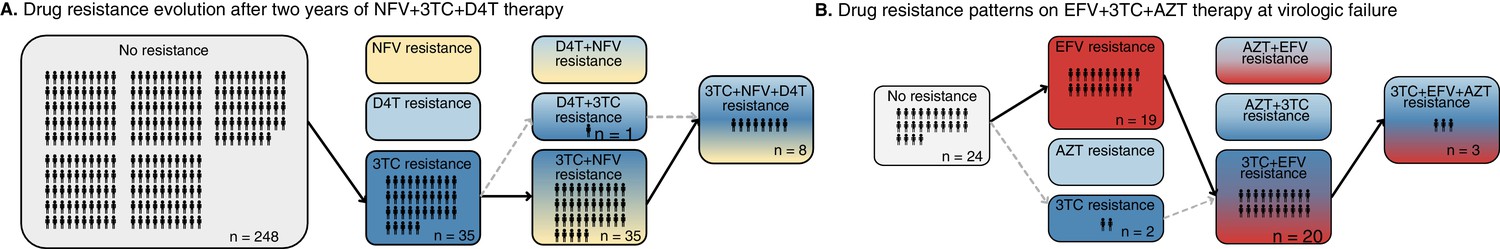
In a clinical trial (M98-863) conducted internationally, 327 participants were randomized to receive treatment with two NRTIs, 3TC (lamivudine) and D4T (stavudine), and a protease inhibitor, NFV (nelfinavir) (Kempf et al., 2004). Patient outcomes from this clinical trial after 2 years are plotted in Figure 1A. We highlight three observations. First, many viral populations evolved drug resistance. Within the first 2 years of therapy, drug resistance was detected in 79 of the 327 patients (24%). Kaplan-Meier plots in the original paper show that roughly half of these cases occurred in the first year of treatment and half in the second year – indicating that standing genetic variation at the start of treatment was not exclusively responsible for treatment failure. Second, drug-resistant viruses were often not resistant to all three drugs in a treatment. Out of these 79 individuals with resistance, approximately half carried resistance to one drug, half carried resistance to two drugs, and eight patients had resistance to three drugs. Third, drug resistance mutations occurred in a seemingly predictable order. All 35 patients with resistance to one drug had resistance to 3TC and 35 of 36 patients with resistance to two drugs had resistance to 3TC and the PI (NFV). While this is cross-sectional data and we cannot observe the order of failure directly, these data strongly suggest that on 3TC+D4T+NFV treatment, drugs fail in a consistent order: 3TC resistance arises first, then NFV resistance, and finally D4T resistance (see Figure 1A).

Figure 1

Download asset Open asset

Patterns of drug resistance evolution in two studies of triple-drug treated individuals with HIV.

(A) Kempf study: Resistance to the drug 3TC emerges first among individuals with HIV taking the triple-drug cocktail NFV + 3TC + D4T (n=327) in Kempf et al., 2004 in a two year study. NFV is a protease inhibitor, and D4T and 3TC are nucleoside reverse transcriptase inhibitors. (B) Hoffman study: Resistance to the drug EFV emerges first among individuals with HIV taking the triple-drug cocktail EFV + 3TC + AZT (n=68) in Hoffmann et al., 2009 . Resistance is reported at the time of virologic failure (≤18 months). EFV is a non-nucleoside reverse transcriptase inhibitor (NNRTI), and AZT and 3TC are nucleoside reverse transcriptase inhibitors (NRTIs). Abbreviations: 3TC: lamivudine, AZT: zidovudine, D4T: stavudine, EFV: efavirenz, NFV: nelfinavir. Solid lines (followed from left to right) represent the most frequent progression of drug resistance, whereas dashed lines represent observed minority paths to resistance.

Hoffman study

A study in South Africa followed patients treated with a common NNRTI-based regimen containing two NRTI drugs, AZT (zidovudine) and 3TC, and one NNRTI, EFV (efavirenz) (Hoffmann et al., 2009). Outcomes for genotyped patients who experienced virologic treatment failure are plotted in Figure 1B. Most of the patients experiencing virologic failure who were genotyped (48/68) had drug resistance mutations. However, similar to the Kempf trial, many of these resistant viral populations had only partially resistant genotypes. Of these genotyped patients, 21 had resistance to just one drug, 20 had resistance to two drugs, and 3 had resistance to all three drugs. Again, the partially resistant populations tended to have predictable compositions: 19 of the singly resistant populations were resistant to EFV (the NNRTI) and just two had resistance to 3TC. All patients resistant to two drugs had resistance to EFV and 3TC. These data strongly suggest that on 3TC+AZT+EFV treatment, drugs again fail in a consistent order, although a different order from the PI-based treatment. Here, EFV failed first (Figure 1B), and 3TC only second, whereas in Kempf et al., 2004, 3TC consistently failed first (Figure 1A).

It is well-known that 3TC resistance can evolve extremely quickly when 3TC is used as a monotherapy (Feder et al., 2021a). 3TC resistance also evolves first when it is co-administered with AZT (Picard et al., 2001; Larder et al., 1995) and as we showed in the previous paragraph, it evolves first when co-administered with D4T and the PI NFV. It is therefore somewhat unexpected that when co-administered with an NNRTI, it appears to not be selected unless NNRTI resistance has already appeared.

Several consistent observations emerge from these two studies: (1) significant resistance evolves despite triple-drug treatments. (2) Viruses do not need to be fully resistant to all drugs in a combination in order to spread to detectable levels within individuals, allowing drug resistance to develop sequentially. (3) Resistance mutations emerge in a partially predictable order. As we discuss below, all three of these patterns are observed much more broadly in larger datasets.

Three key observations of HIV drug resistance evolution during triple-drug therapy

In this section, we look at bigger, yet less detailed, datasets to determine if the observations from the case studies (resistance evolution is ongoing, sequential, and with a partially predictable order) hold more generally.

Drug resistance continues to evolve even after years on successful therapy

Despite triple-drug therapies becoming available in high-income countries in the 1990s, drug resistance evolution remained common. Resistance emerged not only in individuals who had started their treatment before 1995 on mono- or double-drug therapies, but also in individuals who started on a triple-drug regimen in the mid-1990s or later. Several studies (Rocheleau et al., 2018; Phillips et al., 2005) following cohorts of HIV-infected individuals over time found substantial ongoing resistance evolution on both NNRTI-based and PI-based treatments even 5 or more years after starting therapy. In these cohorts, cases of resistance accumulate over time, suggesting that the yearly probability of resistance evolution does not rapidly decline to 0.

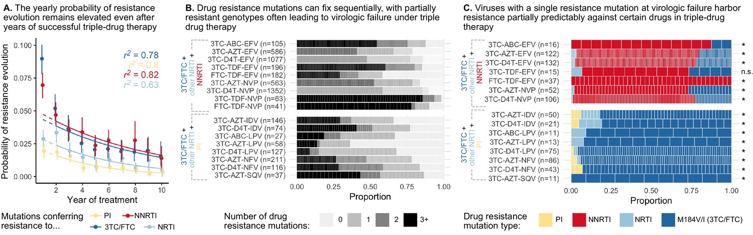
To assess how an individual’s yearly risk of resistance evolution changes after numerous years on combination therapy, we performed a conditional survival analysis on a previously published cohort of HIV-infected individuals from British Columbia in which all people in the province were automatically entered in a provincial registry and received treatment from a central agency free of charge (Montaner et al., 2010; Rocheleau et al., 2018). We computed the yearly probability of resistance evolution in each of the first 10 years of treatment, conditional on no prior resistance evolution up to this point, among 2692 individuals treated with three-drug combination therapies commencing between 1996 and 2005. We observe across all four drug categories (NNRTIs, PIs, non-3TC/FTC NRTIs and 3TC/FTC), the yearly conditional probability of resistance stays elevated above 0 even 5 or more years after the start of therapy (Figure 2A, Supplementary file 2). The conditional survival probabilities are highest in the first year of therapy, and appear to decline thereafter. The point estimates of yearly probability risk are fit well by standard exponential decay for each of the four mutation classes ( $r^{2} = 0.78, 0.80, 0.82, 0.63$ for 3TC, PI, NNRTI and NRTI resistance, respectively) when excluding the first year, which is expected to have a higher rate of failure due to standing genetic variation (Pennings, 2012) or transmitted drug resistance (especially among NNRTIs). The relatively slow rates of decline (Supplementary file 3) suggest that the risk of drug resistance evolution on triple-drug therapy remains even in individuals who have been on successful treatment for years. This highlights the importance of ongoing within-patient processes in treatment failure and suggests that resistance patterns are not driven by a subset of individuals who fail therapy quickly.

Figure 2

Download asset Open asset

Cohort analyses of individuals with HIV reveal drug resistance evolution is ongoing after years on therapy, stepwise and partially predictable.

(A) The yearly probability of resistance evolution conditional on no prior resistance evolution in a large cohort of individuals in British Columbia treated with triple drug therapies (Rocheleau et al., 2018). Conditional evolution probabilities are plotted separately for resistance to 3TC or FTC (dark blue), NNRTIs (red), NRTIs other than 3TC or FTC (light blue) or PIs (yellow). Drug-category specific fits to an exponential model covering years 2–10 and $r^{2}$ describing the model fit are also plotted. Bars represent 95% confidence intervals. (B) Across individuals treated with three-drug combination therapies based on two NRTIs paired with an NNRTI (top) or PI (bottom), many sequences are detected with 0, 1, 2, or 3+ drug resistance mutations in a large cohort (data source: Feder et al., 2016a). (C) In individuals treated with three-drug combination therapies based on two NRTIs paired with an NNRTI (top) who have exactly one resistance mutation, that mutation most often confers resistance to the NNRTI of the treatment (red), although sometimes resistance to 3TC (dark blue) or the other NRTI (light blue) develops. Among individuals treated with a PI paired with 3TC and a second NRTI who have a single drug resistance mutation, that mutation most often confers resistance to 3TC (dark blue), although sometimes it confers resistance to the other NRTI (light blue) or the PI (yellow). Asterisks mark treatments for which the first mutation confers resistance to the NNRTI (top) or 3TC (bottom) more often than expected under the relative mutation probabilities of the three drugs (binomial test, 5% false discovery rate). (Data source: Feder et al., 2016a). Each square in both B and C represents a single individual, and the sample sizes are given next to the treatment names. Abbreviations: abacavir, ABC; indinavir, IDV; lamivudine, 3TC; lopinavir, LPV; nelfinanvir, NFV; stavudine, D4T; saquinavir, SQV; zidovudine, AZT.

Emergence of partially resistant genotypes suggests sequential evolution

Individuals on HIV treatment in high-income countries are tested regularly for viral load. If the viral load is higher than a certain threshold (‘viremia’ or virologic failure), a viral sample will be sequenced and assessed for resistance mutations (Department of Health and Human Services. Panel on Clinical Practices for Treatment of HIV Infection. and Henry J. Kaiser Family Foundation. Panel on Clinical Practices for Treatment of HIV Infection., 2000). Observing sequences with only one or two resistance mutations at this stage suggests that partial resistance can allow growth above the detectable viral load threshold. This is surprising under how we believe triple-drug therapies should work, since a singly-resistant virus should be suppressed by two other drugs and not expand and lead to virologic failure.

In earlier papers, we have mentioned the observation that drug resistance evolves in a step-wise fashion (Pennings et al., 2014; Pennings, 2013), but did not systematically query this effect across a broad range of triple-drug therapies. To understand if this effect is widespread across treatments, we analyzed a large set of HIV sequences (6717 individuals) from the Stanford HIV Drug Resistance Database. The presented sequences stem from samples at detection of viremia on triple-drug therapy. In these sequences, we identified large-effect drug resistance mutations and quantified the number of mutations per sequence (Figure 2B, see methods). While some individuals failed without any detectable drug resistance (likely due to non-adherence), viral populations in many others harbored one, two, three or more resistance mutations. That many sequences harbored only one or two drug resistance mutations suggests that partially resistant virus can replicate in the body and lead to a detectable viral load, even when treated with three drugs. This is consistent with results from Figure 1 showing that resistance mutations accumulate in a seemingly step-wise fashion. Note, viruses with three or more resistance mutations may still have accumulated resistance mutations one at a time but these intermediate steps may not have been captured by sampling.

Drug resistance mutations accumulate in a partially predictable order

Possibly the most surprising observation from our two cases studies is that drug resistance mutations emerge in a particular order. Ordering of mutations in HIV has been noted before for different mutations that confer drug resistance to the same drug (Beerenwinkel et al., 2005a; Beerenwinkel et al., 2005b; Posada-Céspedes et al., 2020; Boucher et al., 1992; Molla et al., 1996). That resistance to one class of drugs tends to precede resistance to another class of drugs has not received much attention in the evolutionary literature. To understand which resistance mutations emerge first on triple-drug therapy, we again examined the Stanford HIV Drug Resistance Database dataset described above and considered only viral populations which harbored a single resistance mutation. For each of those singly resistant populations, we determined the drug to which the mutation conferred resistance (Figure 2C). In individuals on PI-based therapies, the singly-resistant viral populations almost all carry a 3TC-resistance conferring mutation, suggesting that resistance to 3TC overwhelmingly occurs before resistance to either the other NRTI or the PI. This ordering of mutations cannot be explained by different mutational target sizes or mutation rates (computed rates given in Supplementary file 4). For each triple-drug combination, we computed the sum of the mutation rates for all 3TC resistance mutations versus the total rate for resistance mutations for any administered drug to get an expected probability that the first resistance mutation to occur should confer resistance to 3TC. We found that for all therapies, resistance to 3TC occurs more often than predicted (p < 0.05, one-sided binomial test with a Benjamini-Hochberg correction and 5% false discovery rate, Figure 2C, all test details given in Supplementary file 5). This result also cannot be explained by standing genetic variation because the most common 3TC mutation, M184V, incurs a substantial fitness cost (Paredes et al., 2009; Jain et al., 2011), which should make it unlikely to be present as standing genetic variation (Simen et al., 2009). Note, the major 3TC resistance mutation, M184V, also confers some degree of resistance to ABC. Despite this, M184V was counted as a 3TC-resistance conferring mutation when assessing whether 3TC resistance mutations preceded others in the only PI-based, ABC-containing therapy, 3TC+ABC+LPV.

In individuals treated with NNRTI-based therapies, single drug resistance mutations most often conferred resistance to NNRTIs (Figure 2C), suggesting NNRTI resistance occurred first. In performing an analogous test comparing the overall mutation rates toward NNRTI resistance versus the resistance mutation rate for any drug in a treatment, we found that in all therapies except one, NNRTI resistance occurred more often than predicted by the relative mutation rates (one-sided binomial test with 5% FDR and Benjamini-Hochberg correction, Supplementary file 6). The one triple-drug combination where the null hypothesis was not rejected (3TC-TDF-EFV) also had the fewest number of observations ( $n = 15$ ). Note, we can only comment on the first resistance mutation that is actually observed, but it is also possible that other classes of resistance mutations rise to high frequency before the first mutations identified above but these mutations are then outcompeted due to clonal interference.

Collectively, we have presented three observations that can help guide the construction of models: (1) drug resistance evolution was common on triple-drug therapies in the 1990s and 2000s, and even individuals who had been on treatment for several years were still at risk for resistance evolution; (2) resistance evolves in a sequential manner (first one mutation, then a second, then a third, rather than three mutations at the same time), leading to the observation of partially-resistant viruses; (3) mutations emerge in a partially predictable order that cannot be explained by mutational target size. We next describe two potential explanations for drug resistance evolution on triple-drug therapies and explore how they might produce the patterns described above.

Two models of resistance evolution due to drug level heterogeneity

Two types of models have been used to explain how drug resistance emerges on combination therapies: models with temporal heterogeneity in drug concentrations (Rong et al., 2007; Braithwaite et al., 2006; Rosenbloom et al., 2012; Cadosch et al., 2012; Bershteyn and Eckhoff, 2013) and models with spatial heterogeneity in drug concentrations (Kepler and Perelson, 1998; Moreno-Gamez et al., 2015; Sanche et al., 2017). Both models rely on drugs falling below their intended concentrations at certain points in time or space. The literature on temporal heterogeneity is more extensive and includes cohort studies on the adherence-resistance relationship in HIV (Bangsberg et al., 2004; Harrigan et al., 2005). While nobody doubts that spatial and temporal heterogeneity exist, it is not clear if either or both can explain the observed evolutionary patterns.

Before describing in more detail the spatial and temporal heterogeneity models, we first explain why heterogeneity is crucial - namely, HIV drugs work too well at their administered concentrations for ongoing replication. Even when administered as monotherapy, drugs cause sensitive viral populations to shrink (Eron et al., 1995; Reiss et al., 1988). As an example, we plot data from a patient treated with AZT monotherapy (Figure 3A). Initially, the treated viral population shrinks. Only after 16 weeks, the viral population expands again to detectable levels. Measuring the ability of the drug-resistant and sensitive virus to replicate at different drug concentrations (i.e. the Hill dose-response curve, Figure 3B, Chou, 1976; Zhang et al., 2004; Sampah et al., 2011) helps explain the dynamics, and such curves have been measured in cell culture for anti-retroviral-treated HIV (Sampah et al., 2011).

Figure 3

Download asset Open asset

Dose response curves help explain the dynamics of treated viral populations.

(A) HIV antigen levels initially decline when treated with AZT monotherapy (6x200 mg/day) to below a detectable threshold (dotted line). Starting at week 16, the viral population begins to rebound even in the presence of the drug, indicating the evolution of drug resistance. (A) Is reprinted with annotations from Figure 1A from The Lancet, 1 (8582), Reiss et al, ‘Resumption of HIV antigen production during continuous zidovudine treatment’, Page 421, Copyright (1988), with permission from Elsevier. It is not covered by the CC-BY 4.0 licence and further reproduction of this panel would need permission from the copyright holder. (B) Schematic shows different regimes of viral behavior dependent on the concentration of a particular drug. At high concentrations (right side of the plot), both drug-resistant (dashed red) and drug-sensitive (solid black) viruses are suppressed, with R₀ below 1. As drug concentration decreases, a window of concentrations emerges where the drug-resistant virus can grow in population size in the presence of the drug ( $R_{0} > 1$ ), but the drug-sensitive genotype cannot. This is termed the ‘mutant selection window’ (Drlica, 2003). At lowest concentrations, both wild-type (WT) and drug-resistant viruses can replicate, but the WT virus out-competes the drug-resistant type because it does not carry the fitness penalty of costly drug resistance mutations. Labels 1 and 2 show how the dynamics of the population in A can be explained by a mutation which behaves like the black arrow in B. If the drug concentration is higher and the resistance mutation only confers a change in R₀ according to the blue arrow, the viral population will remain suppressed.

© 1988, Elsevier. is reprinted with annotations from Figure 1A from Reiss et al., 1988, Copyright (1988), with permission from Elsevier. It is not covered by the CC-BY 4.0 licence and further reproduction of this panel would need permission from the copyright holder.

At certain intermediate drug concentrations, the resistant mutant can grow ( $R_{0} > 1$ ) and the sensitive strain cannot ( $R_{0} < 1$ ) (Rosenbloom et al., 2012, Figure 3B). Concentrations within this so-called ‘mutant selection window’ (which also includes concentrations at which both sensitive and resistant virus have $R_{0} > 1$ , and $R_{r e s i s t a n t} > R_{s e n s i t i v e}$ , Rosenbloom et al., 2012) select for resistance. The dynamics plotted in Figure 3A suggest AZT concentration falls within this window: the population initially shrinks (Figure 3A, label 1) suggesting the drug-sensitive genotype must have $R_{0} < 1$ (Figure 3B, label 1), but then begins to grow again (Figure 3A, label 2), suggesting that the drug-resistant genotype must be above the $R_{0} = 1$ line (Figure 3B, label 2). In principle, had AZT dosage been higher (e.g. blue arrow in Figure 3B), the resistant virus would be unable to increase in size because its R₀ would be below one despite its resistance. Drugs overpowering even resistant virus at high concentrations have been demonstrated empirically in experimental settings (Sampah et al., 2011).

Combining three drugs that each bring the viral R₀ below 1, should result in an even lower R₀ (although how much lower is not straightforward, see Jilek et al., 2012). Even if a virus acquires a resistance mutation rescuing its ability to replicate in the presence of one drug, as long as the combination of the three drugs suppresses R₀ below 1, that singly resistant virus should not spread. That we see partially resistant viruses reach detectable levels in patients means there must be a time or space where this virus replicates at $R_{0} > 1$ .

Temporal heterogeneity

After a patient takes a dose of treatment, the drugs are absorbed and metabolized within the body, resulting in an increase and then a decrease in drug concentration. Ideally, each drug is dosed such that the viral population cannot replicate under normal daily drug fluctuations (Figure 4A). However, patient non-adherence and different rates of drug metabolism between individuals can lead to drug concentrations that drop below the required levels over time. This has been widely recognized as a potential route to drug resistance (Fox et al., 2008; Bangsberg et al., 2007; Harrigan et al., 2005; Chesney et al., 2000; Cadosch et al., 2012).

Figure 4

Download asset Open asset

Heterogeneity in time or space can allow the spread of drug resistant viruses.

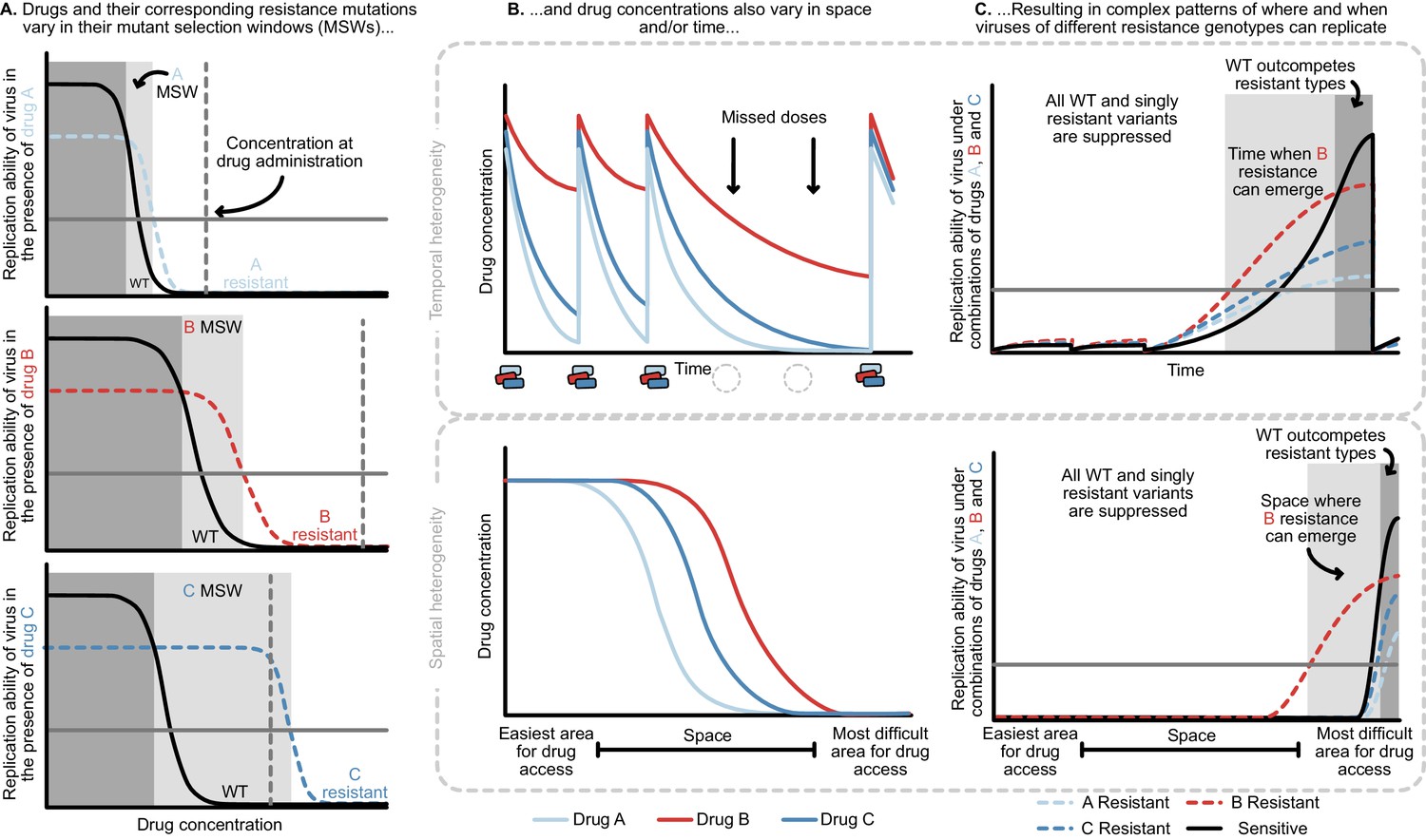
(A) Different drugs and their associated drug resistance mutations have differently shaped concentration response curves and corresponding mutant selection windows (MSW). Pictured here, drug A (light blue) has the smallest MSW, whereas drug C (dark blue) has the widest MSW. Drug B (red) has an intermediate MSW. (B) Variable MSWs also interact with drugs that have heterogeneous concentrations either in time (top) or space (bottom). Missed doses (due to incomplete adherence, plotted on top) can allow only drugs with long half-lives (here, Drug B) to remain present. This can create windows in time (pictured in C) which select resistance to only this longest half-life drug. If drug levels are allowed to decline sufficiently low, viral replication of non-resistant types can emerge as well. Drugs that do not reach all of the body (plotted on bottom) can create areas where single drug resistance mutations (pictured in C) can replicate. Areas where effectively no drugs reach can create a sanctuary where some viral replication of the wild-type (WT) virus can continue.

The mutant selection window provides a useful lens through which to understand the consequences of missed doses. At drug administration, viral populations experience small R₀ values to the right of the mutant selection window and R₀ values increase as drug concentrations decay, moving to the left on the x-axis (Figure 4A). Drugs with short half-lives move quickly to lower concentrations, while drugs with long half-lives may move slowly through their mutant selection windows. Missed doses may result in drug depletion of quickly decaying drugs while slowly decaying drugs may remain in their mutant selection window. This allows virus resistant to the longest half-life drug to replicate. Figure 4B and C show a scenario in which after missed doses, drug B in red with the longest half-life enters the mutant selection window after shorter half-life drugs leave the system. The dynamics clearly depend not just on drug B’s mutant selection window, but also the rate at which all drugs are metabolized. To model this situation, it is therefore critical to incorporate the mutant selection windows, relevant drug interactions and drug concentration dynamics for all drugs.

In addition to understanding drug concentrations and the mutant selection windows, several other considerations are important. If the population size is small due to virologic suppression, mutations that confer resistance may not be present, even if the drug conditions would allow them to spread. Second, for the mutant to be successful, the decrease in virus while the patient is taking drugs must be smaller than the increase in virus during the mutant selection window. Patients missing doses too frequently may not select for resistant virus at all. It is unclear which adherence patterns result in this behavior, and if these same adherence patterns can explain why individuals fail treatment with resistance after 5–10 years on therapy.

We now return to the clinical data and ask whether these patterns may emerge from a model of temporal heterogeneity. Individuals treated with 3TC+D4T+NFV acquire resistance largely in the order of 3TC, then NFV, then D4T. Both NFV and D4T are expected to lose most of their suppression within 24 hr due to short half-lives and, in the case of D4T, low potency (Rosenbloom et al., 2012). If a patient misses a dose, 3TC may quickly be the only potent drug present and enter its mutant selection window, allowing a 3TC-resistant genotype to spread. Indeed, we observe that 3TC mutations dominate over PI mutations among single drug resistance mutations in individuals treated with PI therapy and an NRTI backbone containing 3TC (Figures 1A and 2C).

To test whether a quantitative model could create these expected patterns, we extended an existing model of HIV drug resistance evolution (under a variety of adherences) to include combination therapies. Briefly, we simulated 1500 HIV-infected individuals taking 3TC+D4T+NFV (the therapy examined in Figure 1A) for a ten-year period and recorded when (if at all) viral populations first became clinically detectable, and which resistance mutations (if any) were present (see Materials and methods for full details). Drugs decay over time according to measured half-lives, and viral fitnesses depend on their genotype and the drug levels currently present. Critically, individuals have an underlying adherence level which controls their probability of missing doses at each administration period.

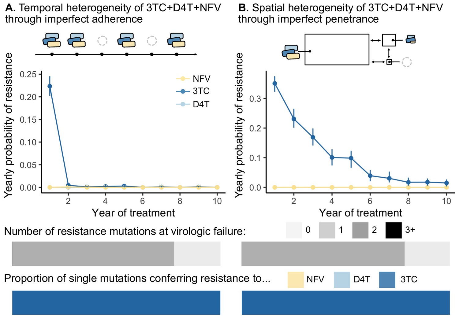
We found that this model of temporal heterogeneity could explain some but not all features observed in the clinical data under three-drug combination therapies. Consistent with clinical observations, resistance mutations often emerge one mutation at a time and can lead to clinically detectable viral loads (Figure 5). This model also produced instances of virologic failure without any resistance mutations, presumably in individuals with particularly poor adherence. Also in agreement with clinical observations, when resistance did evolve, mutations occur in a predictable order and resistance to 3TC always precedes NFV and D4T. In disagreement with clinical observations, we find that resistance overwhelmingly emerges in the first year of treatment when the population size is large, but then falls to quite low levels for the next years. 95.3% of the simulated individuals who did not develop resistance in the first year had suppressed HIV populations for the entire simulated 10-year treatment period. This suggests that under a simple model of non-adherence for 3TC+D4T+NFV, potentially little resistance evolves after initial viral suppression, although we will note in the discussion how more sophisticated models of adherence may more effectively select for resistance.

Figure 5 with 2 supplements see all

Download asset Open asset

Models of spatial and temporal heterogeneity of drug levels explain certain evolutionary patterns observed in clinical data.

Using parameterized models of (A) temporal and (B) spatial heterogeneity of drug levels stemming from imperfect adherence and imperfect penetrance, respectively, we can assess the presence or absence of patterns found in clinical data. First, we plot the yearly probability of resistance evolution conditional on no resistance to this point for 3TC, D4T and NFV for each year of treatment. Bars represent 95% confidence intervals. Second, we plot the proportion of individuals with 0, 1, 2 or 3 resistance mutations at the time of virologic failure ( $n = 446$ under temporal heterogeneity and $n = 1121$ under spatial heterogeneity). Third, we plot the proportion of individuals with resistance to NFV, D4T, or 3TC conditional on having a single resistance mutation at the time of virologic failure ( $n = 346$ under temporal heterogeneity and $n = 878$ under spatial heterogeneity). Note, the cartoon model of spatial heterogeneity in drug levels does not show the compartment sizes to scale.

Above, we simulated a model in which 3TC has the longest half-life in a PI-based drug combination (3TC+D4T+NFV). Unlike PIs, NNRTIs have particularly long half-lives (Taylor et al., 2007). Treatment interruptions of a few days are long enough for non-NNRTIs to leave the system, but short enough for NNRTIs to remain present. We would therefore expect NNRTI resistance to occur first, which is consistent with the data presented in Figures 1A and 2C. However, other data are not consistent with this explanation. An observational study conducted as part of the SMART trial on treatment interruptions tried to prevent a period of NNRTI monotherapy when interrupting treatment (so called staggered or switched stops) by ‘covering’ the tail with additional shorter lived drugs (Fox et al., 2008). It turned out that ‘covering’ the tail did not affect the risk of drug resistance evolution (Fox et al., 2008), suggesting that the tail of NNRTI monotherapy may not be the reason NNRTI drug resistance evolves. We (Pennings) have proposed another explanation, namely that an increase in population size during an interruption allows resistance mutations to accumulate as standing genetic variation. When treatment resumes, these mutations increase in frequency due to selection (Pennings, 2012). Clearly, these observations demand more investigation into how temporal heterogeneity can generate such patterns, and indeed underscore the challenge of thinking about such observations without a quantitative model.

Spatial heterogeneity

HIV drugs do not penetrate throughout the body uniformly and penetration profiles differ among drugs. As a result, even in triple-drug-treated individuals, parts of the body (e.g. brain, lymph nodes) may experience monotherapy (Else et al., 2011; Letendre et al., 2008; Decloedt et al., 2015; Fletcher et al., 2014; Thompson et al., 2019). Under a model of spatial heterogeneity, the concentrations that allow replication and expansion of drug-resistant virus (i.e. the mutant selection window of each drug) are distributed in physical space, as opposed to time. These concentration profiles may be largely overlapping and nesting (as illustrated in Figure 4B) or drugs may have semi-independent penetrance profiles, wherein some drugs reach certain parts of the body effectively, and other drugs reach other parts of the body effectively.

Different penetration profiles may result in parts of the body that consistently have drug concentrations that allow the replication of partially resistant genotypes (Figure 4C). A partially resistant virus migrating or reactivating from the latent reservoir in that part of the body may establish a growing HIV population. Even if these variants can only successfully replicate in one part of the body (i.e. the single drug compartment), they may still lead to a detectable viral load in a blood sample. After establishing in a single drug compartment, variants have the opportunity to acquire additional mutations that allow them to replicate elsewhere. In principle, this can explain the three observations above. First, drug resistance can continue to evolve at rates determined by the population mutation rate and migration rates into such a single-drug compartment even after years of virologic suppression. Second, partially resistant viruses may be observed if replication in one or more single drug compartments can be detected in the blood. Third, drugs with different penetrance profiles can explain why drug resistance evolves in a predictable order - namely in response to the best-penetrating drug first.

As in the temporal heterogeneity model, the spatial heterogeneity model may help us understand qualitative patterns previously observed in clinical trial data. In the Kempf study, patients were treated with 3TC, NFV, and D4T (see Figure 1A), where a plausible 3TC single-drug compartment may exist. 3TC, NFV, and D4T have differential rates of penetrance into the brain, with penetrances of NFV and D4T particularly poor (Letendre et al., 2008; Browne et al., 1993; Aweeka et al., 1999; Ene et al., 2011). This can create parts of the brain where 3TC-resistant HIV can effectively replicate and spread, potentially allowing detection in the blood as a 3TC-resistant type. Once resistant to 3TC, the virus needs only one additional mutation to replicate in the presence of NFV. In practice, because of D4T’s poor potency (Rosenbloom et al., 2012), much of the body may effectively be a 3TC+NFV compartment and select for NFV mutations next (Figure 1A).

To test whether a model of spatial heterogeneity of drug levels can explain the three clinically observed features, we extended a pre-existing model of HIV spatial drug penetrance to account for three drug combinations (Moreno-Gamez et al., 2015). Similar to the temporal model, we simulated 1500 individuals infected with HIV and treated with 3TC+D4T+NFV and followed for up to 10 years. Here, instead of drugs decaying over time, we computed the average drug dose over time in a fully adherent patient, but assumed that drugs do not reach all parts of the body equally. We simulated three compartments interconnected by migration: (1) the majority of the body reached by all three drugs at full concentration, (2) a brain-like compartment reached by all three drugs at lower concentrations according to comparative measurements of drug levels in the plasma and cerebrospinal fluid (CSF) (Ene et al., 2011) and (3) a small sanctuary compartment reached by no drugs. We recorded when the viral population in the main compartment (presumably the measured compartment when assaying viral loads) exceeded a detectable threshold (see Materials and methods).

We found that this model of spatial heterogeneity produced all three features that we observed in the clinical data under three-drug combination therapies, but only for one of the drugs in the combination - 3TC (Figure 5). First, 3TC resistance continues to emerge, even if individuals have been on therapy for several years. This decline in probability over time emerges from the simulated distribution of viral setpoints, which vary between 10⁴ and 10⁶ (interquartile range $7.92 \times 10^{4} - 3.18 \times 10^{5}$ ). Individuals with larger population sizes evolve resistance more rapidly than those with smaller population sizes (Figure 5—figure supplement 1), and simulating a narrower band of viral set points (interquartile range $1.36 \times 10^{5} - 1.71 \times 10^{5}$ ) results in a yearly resistance probability that remains approximately constant over time (Figure 5—figure supplement 2). Second, resistance mutations exclusively emerge one at a time and can lead to clinically detectable levels. Third, resistance mutations occur in a predictable order, and we see overwhelmingly resistance to 3TC and no ongoing resistance to NFV and D4T. We see only 3TC resistance evolve because the penetrance of D4T and NFV in the CSF is sufficiently low that the cost of D4T or NFV resistance dominates over its benefit (i.e. $R_{N F V / D 4 T r e s i s t a n t} < R_{N F V / D 4 T s e n s i t i v e}$ ). This suggests that compartments with additional patterns of drug penetrance are necessary to provoke additional resistance evolution. Even though this simplified model of drug spatial heterogeneity does not capture additional resistance evolution for two drugs in the combination, all three patterns straightforwardly emerge with respect to 3TC resistance (Figure 5).

Above, we examined a PI-based therapy, but a similar spatial model may also explain some of the patterns in NNRTI-based therapies. NNRTIs tend to have strong penetration profiles, which may explain why drug resistance to NNRTIs emerges first (Figures 1B and 2C). However, many NNRTIs are highly suppressive even at relatively low concentrations and sometimes even for genotypes with resistance mutations. This suggests that an NNRTI resistance evolution may require not only a single drug compartment (i.e. the absence of other drugs), but also a sub-clinical concentration of the NNRTI to select for resistance mutations.

For both the spatial and the temporal models there is an interesting and somewhat counter-intuitive effect. Intuitively, one might think that resistance will first arise in response to the ‘worst’ drug in a cocktail (least potent, shortest half-life, or worst penetration profile). However, in a model of spatial or temporal heterogeneity, a desirable property –high penetration or long half-life– actually makes a drug vulnerable to resistance. Therefore, the best way to prevent the evolution of 3TC resistance (when treatment is with 3TC+NFV+D4T) is not to target the shortcomings of 3TC, but to target the shortcomings of the other drugs. Specifically, if 3TC monotherapy occurs in space or time because of a long half-life or good penetration, the solution would be to add another drug that also has a long half-life or good penetration.

The introduction of second generation PIs in the early 2000s resulted in exactly this intervention. In particular, ritonavir-‘boosted’ lopinavir (LPV/r) (Tseng et al., 2015) resulted in improved penetance and extended half-life in comparison to NFV (Capparelli et al., 2005). The clinical effect of replacing NFV with LPV/r in the previously described Kempf study (Kempf et al., 2004) is a substantial reduction of resistance evolution by 76%. In the NFV arm of the study, 79 of 327 individuals developed some type of drug resistance (24%) within 2 years, whereas in the LPV/r arm, only 19 of 326 did (6%).

In the context of resistance evolution via spatially-varying drugs, LPV/r consistently reaches a level above the 50% inhibitory concentration in cerebrospinal fluid (Capparelli et al., 2005), thereby likely shrinking the size or number of compartments in which 3TC exists alone. The fourfold lower rate of drug resistance evolution among individuals on the LPV/r regimen suggests that the enhanced spatial coverage of LPV/r decreased the portions of the body where 3TC reached alone by a factor of four. In the context of resistance evolution via temporally varying drugs, the longer half-life of LPV/r could reduce the time of 3TC as effectively a monotherapy. Future models should test whether differences in drug penetrances or half-lives better explain the reduced rate of resistance with LPV/r treatments.

Discussion

Above we have described ideas about how drug-level heterogeneity in time, due to different half-lives and non-adherence, can lead to periods of monotherapy, which, in principle, can lead to drug resistance evolution during triple-drug therapy. We have also described how heterogeneity in space, due to different penetration profiles of drugs, can lead to single-drug compartments, which also, in principle, can lead to drug resistance evolution. We extended existing one or two drug models for imperfect adherence and imperfect drug penetrance and found that a model of spatial heterogeneity can recreate the observed clinical patterns – ongoing, sequential and predictable evolution – for resistance to specific drugs but not others. A temporal model readily matches certain observations (sequential and predictably ordered mutations), but not others (namely, ongoing resistance after years on therapy). Therefore, we have two possible explanations for the observation that drug resistance can evolve during triple-drug therapies, neither of which currently explain all aspects of the data in their current state. Further, while we know that temporal and spatial heterogeneity exist and can cause drug resistance evolution, this does not prove that they do.

Models that are intuitively convincing need not be true. For example, NNRTIs have long half-lives, which can lead to periods of monotherapy (the so-called ‘NNRTI tail’) if patients miss doses or interrupt treatment. Additionally, HIV often evolves resistance to NNRTIs (Rocheleau et al., 2018). Yet, there is some evidence that the NNRTI tail does not explain NNRTI drug resistance in low-adherence patients (see discussion under temporal heterogeneity). In our model of temporal heterogeneity in drug levels through incomplete adherence (of PIs, not NNRTIs), many individuals stayed virologically suppressed despite poor adherence. Even though drug conditions intermittently select for drug resistant variants, viral populations could not reach critical population sizes rapidly enough to produce the relevant variants that could spread. While outside the scope of this study, we propose that a quantitative approach that includes mutant selection windows, pharmacokinetics and population genetics is needed to adjudicate between potential explanations for a variety of drug combinations. Can we build a model that can quantitatively match the observations?

Detailed models of HIV drug resistance have already been developed, especially for models of temporal heterogeneity. For example, in a carefully parameterized HIV model focused largely on single drugs (Rosenbloom et al., 2012), the authors examined how adherence patterns for a two-drug therapy (boosted darunivir and raltegravir, DRV/r + RAL) affected the mode and rate of resistance evolution. They found that virologic failure could occur from a viral population resistant to raltegravir but not darunivir, because of the characteristics of the darunivir mutant selection window. Similarly, Bershteyn and Eckhoff, 2013 examined drug resistance dynamics in individuals taking PrEP (TDF) under a realistic model of non-adherence. Adherence models that more closely mimic human behavior may allow for ongoing evolution of resistance years after initial virologic suppression, a clinical outcome expected but not observed in our exploration of 3TC+D4T+NFV. However, these analyses of one or two drug combinations served as proofs of concept, and no three-drug therapies were examined. A real gap therefore remains in developing realistic models that can explain complex patterns of resistance emergence under the most widely used triple-drug therapies.

For the spatial models, the gap between the models and clinical data is even larger than for the temporal models, because the models that have been studied are simpler (Perelson et al., 1997; Moreno-Gamez et al., 2015; Lorenzo-Redondo et al., 2016). Filling this gap will be particularly challenging because many parameters remain unknown. Understanding where, when, and how certain drugs reach different parts of the body is complicated (Vendel et al., 2019) and indeed, different studies have found different relative penetrances of drugs into the tissue versus the plasma. In addition, studies of drug penetrance may not be quantifying the correct factors to help us understand where drug resistance can emerge. First, the administered version of a drug may be at a different concentration than the active form (Dumond et al., 2008). Second, the intracellular concentration of a drug, rather than the tissue concentration, may mediate effectiveness, requiring that we understand not only whether drugs reach a tissue, but the rates at which they are transported into cells (Bazzoli et al., 2010; Dumond et al., 2008). Third, we may not be investigating penetrance in the correct compartments, or at the correct spatial scale. For example, there can be considerable heterogeneity of drug penetrance even within a single lymph node or gut cross-section (Thompson et al., 2015; Thompson et al., 2019). Fourth, many studies report tissue drug concentrations relative to the blood plasma, without considering the actual tissue drug level and its inhibitory effect on the virus (Else et al., 2011). Even comparing tissue drug concentration to the IC50 does not capture the full dynamics of drug concentrations within the body (Shen et al., 2008).

For both the spatial and temporal models, differences between people should also be taken into account. For example, treatment with other drugs (e.g. tuberculosis drugs) may affect the half-lives and penetration of HIV drugs (López-Cortés et al., 2002). Genetic variation among treated individuals may also mediate penetrance (see Apostolova et al., 2015). For example, efavirenz concentrations are higher in people with certain genotypes, and these genotypes are more common in Black/African groups. Rates of drug metabolism also differ between men and women (Else et al., 2011). Different adherence patterns could hypothetically make different mutational orderings more or less likely as well. A recent paper suggests that the combination of imperfect adherence with imperfect penetration makes sequential drug resistance evolution likely in an in vitro system (Lustig et al., 2019).

For now, it remains unclear if temporal heterogeneity, spatial heterogeneity, or a combination of the two cause the evolution of drug resistance during triple-drug therapy. Clarity on this important unresolved mystery will aid the rational design of treatments that minimize the risk of resistance evolution.

Mathematical modeling has played an essential role throughout the HIV pandemic, and we do not intend to diminish these accomplishments. Early studies set a gold standard in uniting available measurements of viral populations (most often viral load) with quantitative models to understand many facets of HIV biology (see review in Nowak and May, 2000). Indeed, these studies helped motivate the need for triple-drug therapies in the first place (Perelson and Nelson, 1999). Now, armed with decades of genetic data, we need to continue this work to understand why triple-drug therapy is not evolution-proof.

Future studies addressing the evolution of multi-drug resistance in HIV should use realistic parameters (for example, like Rosenbloom et al., 2012 and Bershteyn and Eckhoff, 2013) and will need to grapple with the pharmacokinetics of multiple drugs and how they interact (Koizumi and Iwami, 2014; Jilek et al., 2012). Experimental work has highlighted drug pairs that suppress in vitro viral populations to both greater and lesser extents than each drug working independently, which may provide a partial answer to why some combinations of drugs fail at a surprisingly high rate (Jilek et al., 2012). These future studies should not just match viral loads and rates of patient failure, but also genetic patterns of resistance. In addition to the patterns described in this paper (ongoing, sequential, and predictable resistance evolution), other observations should be considered: drug resistance rates have fallen over time (Feder et al., 2016a), virologic failure varies as a function of adherence (Harrigan et al., 2005) and between different drug combinations (Lee et al., 2014; Feder et al., 2016a). We hope that expanded models will allow us not only to make predictions – for example, about rates and patterns of resistance for novel combinations of drugs – but also to learn more about HIV’s biology from data we already have. For example, can we use patterns of resistance to estimate how large single-drug compartments are, or how rapidly viruses migrate between different parts of the body (Feder et al., 2019)?

Drug resistance represents a serious threat across disease systems, and spatial and temporal variation in drug levels likely contribute in these other instances as well. For example, while many in the cancer community argue that applying multiple drugs simultaneously should halt the evolution of resistance (Basanta et al., 2012), experimental evidence also suggests multi-drug resistant cells may already exist as standing genetic variation (Bhang et al., 2015). In treated solid tumors, drugs that cannot penetrate through the entire tumor may form a concentration gradient of selection pressure that theoretical (Hermsen et al., 2012; Fu et al., 2015; Gralka et al., 2017) and experimental (Baym et al., 2016) evidence suggests may speed the evolution of resistance. In tuberculosis, there is evidence that drug levels in various types of granulomas are often not as high as in the blood (and do not reach bactericidal levels) (Prideaux et al., 2015), and may be particularly low for some drugs in cavitary lesions (Strydom et al., 2019). Since not all tuberculosis patients have cavitary lesions, this means that ideal drug choice or dosing may not be the same for all individuals (Strydom et al., 2019). Lessons about spatial and temporal heterogeneity in drug concentrations in HIV can form a scaffold upon which we can try to understand resistance evolution in other disease systems.

Even apart from disease, every natural system experiences multiple stressors simultaneously, even if those stressors are less extreme than targeted anti-retrovirals. How populations evolve in response to complex environments represents a fundamental question in evolutionary biology. In addition to (and perhaps because of) its medical relevance, HIV represents a powerful study system for interrogating this question. We understand many of its population parameters relating to viral kinetics, and extensive research has produced a well-developed genotype-phenotype map of resistance mutations. Because drug resistance emerges repeatedly in different individuals, we can understand which features of this intra-patient evolution are generalizable, which provides insights into how evolution mediated by temporally and spatially varying selection pressures occurs.

In theory, multi-drug therapies should suppress pathogen populations and prevent the evolution of resistance. In practice, multi-drug therapies are challenging to achieve, and pathogen populations do not experience all drugs in all places at all times. When diagnosing the failure of any multi-drug approach because of resistance evolution (whether in cancer, antibiotics, herbicides, etc), we suggest the following four guiding questions: (1) Are all drugs effective? (2) Is there cross-resistance? (3) Is there spatial heterogeneity in drug levels? (4) Is there temporal heterogeneity in drug levels? Through understanding the ways that the application of multi-drug therapies falls short of the theory, we are poised to address those shortcomings and decelerate the evolution of resistance.

Materials and methods

Measuring rates of drug resistance evolution over time (Figure 2A)

Request a detailed protocol

To understand how an individual’s probability of acquiring resistance changes over time, we reanalyzed data from a Canadian cohort study (Rocheleau et al., 2018). This is a cohort of individuals with HIV taking combination ART for the first time. We would like to understand the probability that a given individual acquires a drug resistance mutation in a given year, conditional on having acquired no resistance mutations to any class of drugs prior to that year. To estimate this probability, we performed a conditional survival analysis using the R package condSURV (Meira-Machado and Sestelo, 2016). We computed separate estimates for each year following the start of therapy and for each drug resistance mutation class (3TC, NRTI, NNRTI, or PI) for the probability of acquiring a resistance mutation conditional on having acquired no resistance mutations prior to that year. Within each analysis, individuals acquiring a drug resistance mutation for a specific class of drugs were coded as endpoint events, and individuals leaving the study for all other reasons (including resistance to other drugs) were censored. To ensure adequate follow-up time, we analyzed only individuals beginning therapy between 1996 and 2005 ( $N = 2692$ ).

In Figure 2, we fit exponential functions to the conditional survival point estimates for each drug resistance class (3TC, other NRTI, NNRTI, PI) using the formula $f (t) = α e^{β t}$ . Parameter fits for $α$ and $β$ are reported in Supplementary file 3.

Determining the total number of resistance mutations and the first drug resistance mutation on a treatment (Figure 2B and C)

Request a detailed protocol

To determine the number of mutations at sampling and the identity of the first mutation (if present) for a variety of triple-drug therapies, we analyzed data from Feder et al., 2016a representing Sanger-sequenced HIV populations treated with a broad range of regimens between 1989 and 2013 (Stanford HIV Drug Resistance Database). We included only individuals treated with exactly one regimen of three drugs to minimize pre-existing resistance before therapy onset. Ambiguous underlying nucleotide calls (i.e., non-A/T/C/G calls) were interpreted as population polymorphisms among all possible resulting amino acids. For example, an AAS residue (AAC/AAG) was recorded as an asparagine/lysine polymorphism, but an AAY (AAC/AAT) was recorded as asparagine. When multiple sequences were available for the same individual at the same time point, polymorphisms were also recorded.

We then determined the number of drug resistance mutations by comparing sequences to the WHO list of surveillance drug resistance mutations (DRMs) (Shafer et al., 2007). DRMs were only counted if HIV sequences contained residues conferring resistance to the therapy with which they were treated. Two classes of DRMs were recorded: (1) polymorphic DRMs in which some calls supported the DRM and some supported a non-DRM and (2) non-polymorphic DRMs, in which all calls supported the DRM.

To determine the first DRM, we retained only individuals with exactly one polymorphic DRM or exactly one non-polymorphic DRM and any number of polymorphic DRMs (under the assumption that fixed mutations occurred before polymorphic mutations). For individuals with sequences taken at multiple time points, we retained the first sample meeting the conditions above (one polymorphic DRM or one fixed DRM and any number of polymorphic DRMs). In Figure 2B, we plot all three drug treatments with at least 25 individuals. In Figure 2C, we plot all three drug treatments with at least 10 individuals with a single drug resistance mutation.

Testing the enrichment of drug resistance mutation classes in combination therapies (Figure 2C)

Request a detailed protocol

To test the hypothesis that mutations conferring NNRTI resistance occur first on NNRTI-3TC/FTC-NRTI therapies and M184V/I (conferring resistance to 3TC/FTC) occurs first on PI-FTC/3TC-NRTI-based therapies, we first calculated a baseline expectation for the relative rates of resistance emergence for each drug in a three drug combination therapy based on mutation rates alone. We based our calculations on the consensus subtype B sequence provided by the Los Alamos HIV Database (https://www.hiv.lanl.gov/content/index), the WHO list of resistance mutations (Shafer et al., 2007), and mutation rates estimated in Abram et al., 2010. For each relevant amino acid position in protease and reverse transcriptase proteins, we determined all possible one-step mutations. For all one-step mutations, we determined whether they led to resistance to any drugs according to the WHO list. Then, for each drug, we summed the mutation probability for all possible one-step mutations that lead to resistance to that certain drug. The resulting total mutation probabilities ranged from 4 · 10⁻⁵ for TDF to 2 · 10⁻⁴ for LPV. The calculated values are listed in Supplementary file 4.

We then used the drug-specific mutation rates to calculate the expected frequency of resistance to one class of drugs versus the others. Specifically, for NNRTI-based therapies, we divided the sum of the mutation rates for the NNRTI-resistance conferring mutations by the total mutation rate for all of the drug resistance mutations in a given therapy. For PI-based therapies, we divided the mutation rate for 3TC or FTC resistance-conferring mutations by the total mutation rate for all of the drug resistance mutations in a given therapy. We used a one-sided binomial test to determine if the number of individuals with NNRTI resistance or 3TC/FTC resistance as their first mutation was higher than expected by chance on therapies composed of NNRTI-3TC/FTC-NRTI and PI-FTC/3TC-NRTI, respectively. We used a Benjamini-Hochberg correction with a 5% false discovery rate separately for the NNRTI- and PI-based hypotheses. Full details on the tests performed, including the mutation-rate-based null hypotheses for each therapy and the number of successes and failures are listed in Supplementary files 5 and 6.

Modeling temporal heterogeneity (Figure 5A)

We extend the viral dynamics model in Rosenbloom et al., 2012 to consider the application of three drugs simultaneously. In this model, viral particles have a reproductive number $R$ that governs their rate of replication. The presence of drugs alters $R$ as a function of drug concentration, and drug resistance changes the shape of this curve (Figure 3B). Generally, these resistance mutations carry a cost that reduce $R$ , although in the presence of drugs, these drug resistance mutations confer a fitness advantage.

Effect of a drug on viral reproductive number

Request a detailed protocol

Following Rosenbloom et al., 2012, the effect of a drug on viral fitness is computed as a function of the concentration $[x]$ of drug $D$ if the virus does not possess any resistance mutations:

r_{s e n s i t i v e, D} ([x]) = \frac{1}{1 + {(\frac{[x]}{I C_{50, D}})}^{m_{D}}}

and

r_{r e s i s t a n t, D} ([x]) = \frac{(1 - s_{D})}{1 + (\frac{[x]}{ρ_{D} I C_{50, D}})^{m_{D} (1 + σ_{D})}}

if the virus possesses a mutation conferring resistance to drug $D$ . The parameters $ρ_{D}, I C_{50, D}, m_{D}, s_{D}, h_{D}$ and $C_{m a x, D}$ (see below for $C_{m a x, D}$ and $h_{D}$ ) are specific to particular drug/mutation combinations (Rosenbloom et al., 2012), and are given in Supplementary file 7. Since multiple drug resistance mutations confer resistance to a given drug, we created a single composite drug resistance mutation with the most favorable attributes for drug resistance evolution of all possible single-step resistance mutations - that is, highest mutation rate µ, lowest cost of resistance $s$ , highest ρ and lowest σ (following Rosenbloom et al., 2012). For NFV, this resistance mutation ends up equivalent to D30N and for D4T, this resistance mutation ends up equivalent to M41L. For 3TC, this resistance mutation is equivalent to M184V with a slightly lower cost of resistance (0.41 versus 0.46) taken from K65R. Therefore, the basic reproductive ratio of a virus of genotype $i$ in the presence of drug $D$ at concentration $[x]$ is as follows:

r_{i, D} ([x]) = {\begin{cases} r_{s e n s i t i v e, D} ([x]) i f i i s s e n s i t i v e t o D \\ r_{r e s i s t a n t, D} ([x]) i f i i s r e s i s t a n t t o D \end{cases} .

To determine the relevant drug concentration some number of hours after dosing, we assume that the drug decays exponentially from a maximum concentration $C_{m a x, D}$ at 0 hours after dosing with half-life $h_{D}$ :

c_{D} (t) = C_{m a x, D} 2^{- t / h_{D}} .

This is evaluated in half hour increments to compute the concentration of each drug over time.

To simulate lack of adherence, at each dosing period, an individual does not take the required drugs with probability $p$ . Failure to take a dose is evaluated separately for each drug, following Rosenbloom et al., 2012. Additionally, to simulate longer blocks of non-adherence related to failures to fill prescriptions, each year, individuals also have a $p$ probability of an additional two week treatment interruption with no doses taken (following ideas discussed in Bershteyn and Eckhoff, 2013). We model the adherence probability $p$ to be uniformly distributed between 0 and 1, although empirical measurements suggest the distribution should be weighted more heavily toward higher adherences (Bangsberg et al., 2006).

We compute the basic reproductive ratio of genotype $i$ at time $t$ under a combination of multiple drugs as the product of the reproductive numbers against individual treatments times a scaling factor R₀₀ ( $R_{00} = 10$ , following Rosenbloom et al., 2012):

R (i, t) = R_{00} \prod_{D \in (3 T C, D 4 T, N F V)} r_{i, D} (C_{D} (t)) .

This formulation assumes that the drugs affect viral fitness Bliss-independently. Jilek et al., 2012 has measured that 3TC and D4T combine to be more potent than Bliss-independence, but NFV/3TC and NFV/D4T combinations are less potent than Bliss-independence (although more potent than Loewe additivity), suggesting that Bliss-independence is a reasonable assumption for the three drug combination therapy. Equation 4 allows us to compute the basic reproductive number for all eight genotypes (conferring resistance to all combinations of 0, 1, 2, or 3 drugs) at all points in time.

Stochastic simulation algorithm

Request a detailed protocol

Model setup

Request a detailed protocol

First, we determine when a completely adherent individual would take all doses for a 10 year period. Note, 3TC and D4T are dosed twice a day, and NFV is dosed three times a day. We then binomially sample which doses the individual misses based on their adherence probability $p$ , and compute the corresponding drug concentrations for all three drugs at all half hour intervals following Equation 3. From these drug concentrations, we compute the basic reproductive ratio for each of the eight genotypes at each half hour interval following Equation 4.

We next determine the frequency of drug resistance mutations as standing genetic variation in the viral reservoir established before the application of drugs. The frequency of each mutation is determined by the ratio between the rate at which it is produced via mutation ( $μ_{D}$ ) and its cost in the absence of the drug ( $s_{D}$ ), or ‘mutation-selection balance’ ( $f_{D} = μ_{D} / s_{D}$ ). The frequency of the drug-sensitive allele for a given drug $D$ is $1 - f_{D}$ . We determine the frequency of the eight combinations of drug resistance mutations in the reservoir, $f$ , by computing the product of the three drug resistant or sensitive allele frequencies at mutation-selection balance for a given genotype $i$ . Note, stochastic effects result in mutational frequencies that can vary substantially around $μ / s$ (Hermisson and Pennings, 2017), but this stochasticity is not incorporated here. The initial population size of each of the eight genotypes is set to be $y (0) = f * N_{e}$ , rounded to the nearest integer, where $N_{e}$ is drawn from a lognormal distribution. To generate values of $N_{e}$ , we draw an exponent from a normal distribution with mean 5.17 and standard deviation 0.5, and exponentiate 10 by this value. This distribution is centered on the estimated short-term viral effective population size, 1.5 × 10⁵ (Pennings et al., 2014), but varies to reflect individual variation (first decile: 7.5 * 10⁴, ninth decile: 3.3 × 10⁵). We redraw any population sizes less than 10⁴ or greater than 10⁶.

Iterated step

Request a detailed protocol

At each timestep of length 30 min ( $Δ t = 0.02$ ), a Poisson-distributed number of cells of each genotype, e_i, emerges from the latent reservoir with mean proportional to the genotype’s frequency in the reservoir f_i:

e_{i} \sim P o i s s o n (A Δ t f_{i}) .

$A$ represents the number of cells expected to reactivate from the latent reservoir in a day, and we set $A = 3000$ following Rosenbloom et al., 2012.

Each of eight genotypes $i$ produces a Poisson distributed number of newly infected cells (n_i) with mean

n_{i} \sim Δ t (\frac{λ R (i, t) d_{y} y_{i}}{λ + \sum_{j = 1}^{n} R (j, t) d_{y} y_{j}})

where $R (i, t)$ is computed as in Equation 4, d_y represents the death rate ( $d_{y} = 1$ , representing a average lifespan of 1 day), and $λ = N_{e} * R_{00} / (R_{00} - 1)$ (Rosenbloom et al., 2012). Each of these newly infected cells has a probability of mutating to acquire or lose drug resistance to drug $D$ according to mutation rate $μ_{D}$ independently at each of its three loci. We use $m u t_{i \to j}$ to denote the number of cells mutating from genotype $i$ to genotype $j$ at the point of infection.

Before cell death, the number of actively infected cells of genotype $i$ is given as follows:

a_{i} = y_{i} (t) + e_{i} + n_{i} + \sum_{j} m u t_{j \to i} - \sum_{j} m u t_{i \to j} .

Each cell has probability of dying $p = (1 - e^{- d y Δ t})$ , resulting in $d_{i} \sim b i n o m (p, a_{i})$ deaths of cells of genotype $i$ . Therefore, the number of cells of genotype $i$ after one simulation step is given as follows:

y_{i} (t + δ t) = a_{i} - d_{i} .

End condition

Request a detailed protocol

Patients are evaluated every 3 months (12 weeks) for 10 years (480 weeks). If the patient had more than 5000 actively infected cells at an evaluation time point (indicating a substantial increase above baseline reservoir reactivation), the viral population was assessed to have undergone virologic rebound, and the simulation is halted. At each of the three drug resistance loci, drug resistance mutations were recorded if they comprised at least 15% of the population.

Modeling spatial heterogeneity (Figure 5B)

The spatial model analyzed extends Moreno-Gamez et al., 2015 to consider the application of three simultaneous drugs. We also used more realistic fitness values (described above) which reflect that even drug resistant viruses have reduced fitness in the presence of therapy. In this model, we simulate three compartments with different degrees of drug penetrance: (1) a main compartment where all three drugs are present with a carrying capacity $K$ drawn from a log-normal distribution as described above, (2) a brain-like compartment with reduced drug concentration according to experimental measurements (Ene et al., 2011, Supplementary file 7) [because cerebrospinal fluid represents approximately 3% of the plasma volume, this second compartment is 3% of the size of the first compartment], and (3) a sanctuary compartment where no drugs reach, which is 1% of $K$ . Note, the true sizes of these compartments are unknown. In Figure 5—figure supplement 2, we also simulate $K$ drawn from a narrower distribution with an exponent (base 10) drawn from a normal distribution with mean 5.17 and standard deviation 0.05 (an order of magnitude smaller than the standard deviation of 0.5 simulated in Figure 5B).

Unlike the temporal model, we assume for the spatial model that drug levels are constant throughout therapy, and are set to be the average drug levels across a single dosing period in an individual with perfect adherence (see Supplementary file 7 for reference values). We compute the average drug level over a full dosing period ( $t_{D} =$ 12 hr for 3TC and D4T, 8 hr for NFV):

ϵ_{D} = 1 - t_{D}^{- 1} \int_{0}^{t_{D}} c_{D} (t) 𝑑 t .

Effect of a drug on viral reproductive number

Request a detailed protocol

Because the virus can be resistant or sensitive to each of three drugs, there are eight relevant genotypes. In each of the three drug compartments, we compute the effective reproductive number of all eight genotypes given the levels of drugs present. For a virus with genotype $i$ in a compartment $j \in$ (Sanctuary, CSF, Plasma), $R$ is computed as follows:

\begin{aligned} R (i, Sanctuary) & = R_{00} \prod_{3 T C, D 4 T, N F V} r_{i, D} (0) \\ R (i, CSF) & = R_{00} \prod_{3 T C, D 4 T, N F V} r_{i, D} (p_{D} [ϵ_{D}]) \\ R (i, Plasma) & = R_{00} \prod_{3 T C, D 4 T, N F V} r_{i, D} ([ϵ_{D}]) \end{aligned}

where $r_{i, j} ([x])$ represents the ability of genotype $i$ to replicate in the presence of drug $j$ at concentration $[x]$ (Equation 5), $ϵ_{D}$ represents the drug level in a compartment (Equation 9) and $p_{D}$ represents the average proportion of plasma drug concentrations for drug $D$ measured in the CSF (Ene et al., 2011). As in the temporal model, $R_{00} = 10$ . Drug-specific model parameters are given in Supplementary file 7.

Stochastic simulation algorithm

Request a detailed protocol

Model setup

Request a detailed protocol

We instantiate the simulations with the sanctuary compartment at carrying capacity, and the other two compartments empty. No resistance mutations are present in the initial population.

Iterated step

Request a detailed protocol

The rate of an event is $α_{i, j, k}$ , where $i = {0, 1, 2, 3, 4, 5, 6, 7}$ is the genotype of the cell undergoing the event (wildtype, 3TC resistant, D4T resistant, NFV resistant, 3TC+D4T resistant, 3TC+NFV resistant, D4T+NFV resistant, 3TC+D4T+NFV resistant), $j = {0, 1, 2}$ corresponds to the compartment in which the event will occur (plasma, CSF, sanctuary) and $k = {0, 1, 2}$ corresponds to the type of event - replication, death or migration. $α_{i, j, k} = N_{i, j} * λ_{i, j, k}$ , where $N_{i, j}$ is the number of cells of a type in a given compartment and $λ_{i, j, k}$ is the rate at which event $k$ occurs for cells of type $i$ in compartment $j$ .

If $k = 0$ , the virus infects a new cell, which happens with rate $λ_{i, j, 0}$ computed as in equation 10. Three random uniform numbers $X_{A}, X_{B}, X_{C} \in [0, 1]$ are drawn, corresponding to potential mutations to drugs $A$ , $B$ and $C$ . For each drug $D$ , if $X_{D} < μ_{D}$ , the virus mutates from genotype $i$ to the alternative resistance state for the given drug $i^{'}$ . This allows both back mutation, and multiple resistance mutations to emerge in a single round of replication. $N_{i, j}$ is decremented and $N_{i^{'}, j}$ is incremented.
If $k = 1$ , the cell dies, which happens with rate $λ_{i, j, 1} = 1$ , and $N_{i, j}$ decreases by 1.
If $k = 2$ the cell migrates from compartment $j$ to an alternate compartment $j^{'}$ with equal probability, which happens with rate $λ_{i, j, 2} = 0.1$ (approximately the estimated plasma to lymph migration rate in Feder et al., 2019). In the case of migration, $N_{i, j}$ decreases by 1 and $N_{i, j^{'}}$ increases by 1. Once a cell has been selected to migrate, it migrates to an alternate compartment with equal probability.

If the evaluation of an event causes a compartmental population size to grow larger than the compartment-specific carrying capacity, cells in that compartment are downsampled multinomially so that the carrying capacity is enforced.

End condition

Request a detailed protocol

Patients are evaluated every 3 months (12 weeks) for 10 years (480 weeks). If the patient has more than 150 actively infected cells at an evaluation time point, the viral population was assessed to have undergone virologic rebound, and the simulation is halted. The reasoning for this end condition is as follows: the viral setpoint is approximately 10⁵ copies/mL and is readily detectable in the blood. 100 copies/mL is an approximate cutoff for detectable virus in the blood, and is 0.1% of the viral setpoint. We therefore used a cutoff 0.1% of the average simulated effective population size as a detectability threshold. At each of the three drug resistance loci, drug resistance mutations were recorded if they comprised at least 15% of the population.

Code availability

Request a detailed protocol

Code to run all data analysis and simulations is available at https://github.com/federlab/HIV-MDR-evolution/ (Feder et al., 2021b). Data to reproduce Figure 3B and C is from Feder et al., 2016a and is also available on GitHub (Feder et al., 2016b).

Data availability

Data to reproduce Figure 3A is protected patient information, but code to run the analysis is available at the GitHub URL below and the script output (which is plotted in Figure 2A) is available in Supplementary file 2. Data to reproduce Figure 3B and C is from Feder et al, 2016, and is also available on GitHub: https://github.com/affeder/HIV-DRM-sweeps/blob/master/dat/dataset.01.24.txt. Code to reproduce all analyses is available on GitHub: https://github.com/federlab/HIV-MDR-evolution (copy archived at https://archive.softwareheritage.org/swh:1:rev:ae825d43929d9334d6b0aa41695956cf4492dccf).

References

1. Abram ME
2. Ferris AL
3. Shao W
4. Alvord WG
5. Hughes SH
(2010) Nature, position, and frequency of mutations made in a single cycle of HIV-1 replication
Journal of Virology 84:9864–9878.
https://doi.org/10.1128/JVI.00915-10
- PubMed
- Google Scholar
(2015) Efavirenz and the CNS: what we already know and questions that need to be answered
Journal of Antimicrobial Chemotherapy 70:2693–2708.
https://doi.org/10.1093/jac/dkv183
- PubMed
- Google Scholar
(1999) Failure to detect nelfinavir in the cerebrospinal fluid of HIV-1--infected patients with and without AIDS dementia complex
Journal of Acquired Immune Deficiency Syndromes and Human Retrovirology 20:39–43.
https://doi.org/10.1097/00042560-199901010-00006
- PubMed
- Google Scholar
(2004) Paradoxes of adherence and drug resistance to HIV antiretroviral therapy
Journal of Antimicrobial Chemotherapy 53:696–699.
https://doi.org/10.1093/jac/dkh162
- PubMed
- Google Scholar
1. Bangsberg DR
2. Acosta EP
3. Gupta R
4. Guzman D
5. Riley ED
6. Harrigan PR
7. Parkin N
8. Deeks SG
(2006) Adherence-resistance relationships for protease and non-nucleoside reverse transcriptase inhibitors explained by virological fitness
AIDS 20:223–231.
https://doi.org/10.1097/01.aids.0000199825.34241.49
- PubMed
- Google Scholar
(2007) Adherence-resistance relationships to combination HIV antiretroviral therapy
Current HIV/AIDS Reports 4:65–72.
https://doi.org/10.1007/s11904-007-0010-0
- PubMed
- Google Scholar
(2012) Exploiting evolution to treat drug resistance: combination therapy and the double bind
Molecular Pharmaceutics 9:914–921.
https://doi.org/10.1021/mp200458e
- PubMed
- Google Scholar
1. Baym M
2. Lieberman TD
3. Kelsic ED
4. Chait R
5. Gross R
6. Yelin I
7. Kishony R
(2016) Spatiotemporal microbial evolution on antibiotic landscapes
Science 353:1147–1151.
https://doi.org/10.1126/science.aag0822
- PubMed
- Google Scholar
1. Bazzoli C
2. Jullien V
3. Le Tiec C
4. Rey E
5. Mentré F
6. Taburet AM
(2010) Intracellular pharmacokinetics of antiretroviral drugs in HIV-Infected patients, and their correlation with drug action
Clinical Pharmacokinetics 49:17–45.
https://doi.org/10.2165/11318110-000000000-00000
- PubMed
- Google Scholar
1. Beerenwinkel N
2. Däumer M
3. Sing T
4. Rahnenfuhrer J
5. Lengauer T
6. Selbig J
7. Hoffmann D
8. Kaiser R
(2005a) Estimating HIV evolutionary pathways and the genetic barrier to drug resistance
The Journal of Infectious Diseases 191:1953–1960.
https://doi.org/10.1086/430005
- PubMed
- Google Scholar
(2005b) Learning multiple evolutionary pathways from cross-sectional data
Journal of Computational Biology 12:584–598.
https://doi.org/10.1089/cmb.2005.12.584
- PubMed
- Google Scholar
1. Bershteyn A
2. Eckhoff PA
(2013) A model of HIV drug resistance driven by heterogeneities in host immunity and adherence patterns
BMC Systems Biology 7:11–16.
https://doi.org/10.1186/1752-0509-7-11
- PubMed
- Google Scholar
1. Bhang HE
2. Ruddy DA
3. Krishnamurthy Radhakrishna V
4. Caushi JX
5. Zhao R
6. Hims MM
7. Singh AP
8. Kao I
9. Rakiec D
10. Shaw P
11. Balak M
12. Raza A
13. Ackley E
14. Keen N
15. Schlabach MR
16. Palmer M
17. Leary RJ
18. Chiang DY
19. Sellers WR
20. Michor F
21. Cooke VG
22. Korn JM
23. Stegmeier F
(2015) Studying clonal dynamics in response to Cancer therapy using high-complexity barcoding
Nature Medicine 21:440–448.
https://doi.org/10.1038/nm.3841
- PubMed
- Google Scholar
1. Boucher CA
2. O'Sullivan E
3. Mulder JW
4. Ramautarsing C
5. Kellam P
6. Darby G
7. Lange JM
8. Goudsmit J
9. Larder BA
(1992) Ordered appearance of zidovudine resistance mutations during treatment of 18 human immunodeficiency virus-positive subjects
Journal of Infectious Diseases 165:105–110.
https://doi.org/10.1093/infdis/165.1.105
- PubMed
- Google Scholar
(2006) Explaining variability in the relationship between antiretroviral adherence and HIV mutation accumulation
Journal of Antimicrobial Chemotherapy 58:1036–1043.
https://doi.org/10.1093/jac/dkl386
- PubMed
- Google Scholar
1. Browne MJ
2. Mayer KH
3. Chafee SB
4. Dudley MN
5. Posner MR
6. Steinberg SM
7. Graham KK
8. Geletko SM
9. Zinner SH
10. Denman SL
(1993) 2',3'-didehydro-3'-deoxythymidine (d4T) in patients with AIDS or AIDS-related complex: a phase I trial
Journal of Infectious Diseases 167:21–29.
https://doi.org/10.1093/infdis/167.1.21
- PubMed
- Google Scholar
(2012) Assessing the impact of adherence to anti-retroviral therapy on treatment failure and resistance evolution in HIV
Journal of the Royal Society Interface 9:2309–2320.
https://doi.org/10.1098/rsif.2012.0127
- Google Scholar
(2005) Lopinavir concentrations in cerebrospinal fluid exceed the 50% inhibitory concentration for HIV
AIDS 19:949–952.
https://doi.org/10.1097/01.aids.0000171409.38490.48
- PubMed
- Google Scholar
(2000) Adherence to HIV combination therapy
Social Science & Medicine 50:1599–1605.
https://doi.org/10.1016/S0277-9536(99)00468-2
- PubMed
- Google Scholar
1. Chou TC
(1976) Derivation and properties of Michaelis-Menten type and hill type equations for reference ligands
Journal of Theoretical Biology 59:253–276.
https://doi.org/10.1016/0022-5193(76)90169-7
- PubMed
- Google Scholar
(2015) Central nervous system penetration of antiretroviral drugs: pharmacokinetic, pharmacodynamic and pharmacogenomic considerations
Clinical Pharmacokinetics 54:581–598.
https://doi.org/10.1007/s40262-015-0257-3
- PubMed
- Google Scholar
1. Department of Health and Human Services. Panel on Clinical Practices for Treatment of HIV Infection.
2. Henry J. Kaiser Family Foundation. Panel on Clinical Practices for Treatment of HIV Infection.
(2000) Guidelines for the use of antiretroviral agents in HIV-infected adults and adolescents, January 28, 2000 by the panel on clinical practices for treatment of HIV infection
HIV Clinical Trials 1:60–110.
https://doi.org/10.1310/hct.2000.1.1.008
- PubMed
- Google Scholar
1. Drlica K
(2003) The mutant selection window and antimicrobial resistance
Journal of Antimicrobial Chemotherapy 52:11–17.
https://doi.org/10.1093/jac/dkg269
- PubMed
- Google Scholar
1. Dumond JB
2. Reddy YS
3. Troiani L
4. Rodriguez JF
5. Bridges AS
6. Fiscus SA
7. Yuen GJ
8. Cohen MS
9. Kashuba AD
(2008) Differential extracellular and intracellular concentrations of zidovudine and lamivudine in semen and plasma of HIV-1-infected men
JAIDS Journal of Acquired Immune Deficiency Syndromes 48:156–162.
https://doi.org/10.1097/QAI.0b013e31816de21e
- PubMed
- Google Scholar
1. Else LJ
2. Taylor S
3. Back DJ
4. Khoo SH
(2011) Pharmacokinetics of antiretroviral drugs in anatomical sanctuary sites: the male and female genital tract
Antiviral Therapy 16:1149–1167.
https://doi.org/10.3851/IMP1919
- PubMed
- Google Scholar
(2011)
How much do antiretroviral drugs penetrate into the central nervous system?

Journal of Medicine and Life 4:432.
- PubMed
- Google Scholar
(1995) Treatment with lamivudine, zidovudine, or both in HIV-positive patients with 200 to 500 CD4+ cells per cubic millimete
New England Journal of Medicine 333:1662–1669.
https://doi.org/10.1056/NEJM199512213332502
- PubMed
- Google Scholar
1. Feder AF
2. Rhee SY
3. Holmes SP
4. Shafer RW
5. Petrov DA
6. Pennings PS
(2016a) More effective drugs lead to harder selective sweeps in the evolution of drug resistance in HIV-1
eLife 5:e10670.
https://doi.org/10.7554/eLife.10670
- PubMed
- Google Scholar
Software
1. Feder AF
2. Rhee SY
3. Holmes SP
4. Petrov DA
5. Pennings PS
(2016b) HIV drug resistance in drug naive patients, version 6aed7af
GitHub.

https://github.com/affeder/HIV-DRM-sweeps/blob/master/dat/dataset.01.24.txt
(2019) Evolutionary dynamics in structured populations under strong population genetic forces
G3: Genes, Genomes, Genetics 9:3395–3407.
https://doi.org/10.1534/g3.119.400605
- PubMed
- Google Scholar
(2021a) The clarifying role of time series data in the population genetics of HIV
PLOS Genetics 17:e1009050.
https://doi.org/10.1371/journal.pgen.1009050
- PubMed
- Google Scholar
Software
(2021b) HIV-MDR-evolution
Software Heritage.

https://github.com/federlab/HIV-MDR-evolution
1. Fletcher CV
2. Staskus K
3. Wietgrefe SW
4. Rothenberger M
5. Reilly C
6. Chipman JG
7. Beilman GJ
8. Khoruts A
9. Thorkelson A
10. Schmidt TE
11. Anderson J
12. Perkey K
13. Stevenson M
14. Perelson AS
15. Douek DC
16. Haase AT
17. Schacker TW
(2014) Persistent HIV-1 replication is associated with lower antiretroviral drug concentrations in lymphatic tissues
PNAS 111:2307–2312.
https://doi.org/10.1073/pnas.1318249111
- PubMed
- Google Scholar
1. Fox Z
2. Phillips A
3. Cohen C
4. Neuhaus J
5. Baxter J
6. Emery S
7. Hirschel B
8. Hullsiek KH
9. Stephan C
10. Lundgren J
11. SMART Study Group
(2008) Viral resuppression and detection of drug resistance following interruption of a suppressive non-nucleoside reverse transcriptase inhibitor-based regimen
AIDS 22:2279–2289.
https://doi.org/10.1097/QAD.0b013e328311d16f
- PubMed
- Google Scholar
(2015) Spatial heterogeneity in drug concentrations can facilitate the emergence of resistance to Cancer therapy
PLOS Computational Biology 11:e1004142.
https://doi.org/10.1371/journal.pcbi.1004142
- PubMed
- Google Scholar
(2017) Convection shapes the trade-off between antibiotic efficacy and the selection for resistance in spatial gradients
Physical Biology 14:045011.
https://doi.org/10.1088/1478-3975/aa7bb3
- PubMed
- Google Scholar
1. Günthard HF
2. Calvez V
3. Paredes R
4. Pillay D
5. Shafer RW
6. Wensing AM
7. Jacobsen DM
8. Richman DD
(2019) Human immunodeficiency virus drug resistance: 2018 recommendations of the international antiviral Society-USA panel
Clinical Infectious Diseases 68:177–187.
https://doi.org/10.1093/cid/ciy463
- PubMed
- Google Scholar
(1997) A controlled trial of two nucleoside analogues plus indinavir in persons with human immunodeficiency virus infection and CD4 cell counts of 200 per cubic millimeter or less
New England Journal of Medicine 337:725–733.
https://doi.org/10.1056/NEJM199709113371101
- PubMed
- Google Scholar
1. Harrigan PR
2. Hogg RS
3. Dong WW
4. Yip B
5. Wynhoven B
6. Woodward J
7. Brumme CJ
8. Brumme ZL
9. Mo T
10. Alexander CS
11. Montaner JS
(2005) Predictors of HIV drug-resistance mutations in a large antiretroviral-naive cohort initiating triple antiretroviral therapy
The Journal of Infectious Diseases 191:339–347.
https://doi.org/10.1086/427192
- PubMed
- Google Scholar
1. Hermisson J
2. Pennings PS
(2017) Soft sweeps and beyond: understanding the patterns and probabilities of selection footprints under rapid adaptation
Methods in Ecology and Evolution 8:700–716.
https://doi.org/10.1111/2041-210X.12808
- Google Scholar
1. Hermsen R
2. Deris JB
3. Hwa T
(2012) On the rapidity of antibiotic resistance evolution facilitated by a concentration gradient
PNAS 109:10775–10780.
https://doi.org/10.1073/pnas.1117716109
- PubMed
- Google Scholar
1. Hoffmann CJ
2. Charalambous S
3. Sim J
4. Ledwaba J
5. Schwikkard G
6. Chaisson RE
7. Fielding KL
8. Churchyard GJ
9. Morris L
10. Grant AD
(2009) Viremia, resuppression, and time to resistance in human immunodeficiency virus (HIV) subtype C during first-line antiretroviral therapy in South Africa
Clinical Infectious Diseases 49:1928–1935.
https://doi.org/10.1086/648444
- PubMed
- Google Scholar
1. Hogg RS
2. Yip B
3. Kully C
4. Craib KJ
5. Schechter MT
6. Montaner JS
7. Montaner JS
(1999)
Improved survival among HIV-infected patients after initiation of triple-drug antiretroviral regimens

CMAJ 160:659–665.
- PubMed
- Google Scholar
1. Jain V
2. Sucupira MC
3. Bacchetti P
4. Hartogensis W
5. Diaz RS
6. Kallas EG
7. Janini LM
8. Liegler T
9. Pilcher CD
10. Grant RM
11. Cortes R
12. Deeks SG
13. Hecht FM
(2011) Differential persistence of transmitted HIV-1 drug resistance mutation classes
The Journal of Infectious Diseases 203:1174–1181.
https://doi.org/10.1093/infdis/jiq167
- PubMed
- Google Scholar
1. Jilek BL
2. Zarr M
3. Sampah ME
4. Rabi SA
5. Bullen CK
6. Lai J
7. Shen L
8. Siliciano RF
(2012) A quantitative basis for antiretroviral therapy for HIV-1 infection
Nature Medicine 18:446–451.
https://doi.org/10.1038/nm.2649
- PubMed
- Google Scholar
1. Kempf DJ
2. King MS
3. Bernstein B
4. Cernohous P
5. Bauer E
6. Moseley J
7. Gu K
8. Hsu A
9. Brun S
10. Sun E
(2004) Incidence of resistance in a double-blind study comparing lopinavir/ritonavir plus stavudine and lamivudine to nelfinavir plus stavudine and lamivudine
The Journal of Infectious Diseases 189:51–60.
https://doi.org/10.1086/380509
- PubMed
- Google Scholar
1. Kepler TB
2. Perelson AS
(1998) Drug concentration heterogeneity facilitates the evolution of drug resistance
PNAS 95:11514–11519.
https://doi.org/10.1073/pnas.95.20.11514
- PubMed
- Google Scholar
1. Koizumi Y
2. Iwami S
(2014) Mathematical modeling of multi-drugs therapy: a challenge for determining the optimal combinations of antiviral drugs
Theoretical Biology and Medical Modelling 11:1–9.
https://doi.org/10.1186/1742-4682-11-41
- PubMed
- Google Scholar
(1989) HIV with reduced sensitivity to zidovudine (AZT) isolated during prolonged therapy
Science 243:1731–1734.
https://doi.org/10.1126/science.2467383
- PubMed
- Google Scholar
(1995) Potential mechanism for sustained antiretroviral efficacy of AZT-3TC combination therapy
Science 269:696–699.
https://doi.org/10.1126/science.7542804
- PubMed
- Google Scholar
1. Larder BA
2. Kemp SD
(1989) Multiple mutations in HIV-1 reverse transcriptase confer high-level resistance to zidovudine (AZT)
Science 246:1155–1158.
https://doi.org/10.1126/science.2479983
- PubMed
- Google Scholar
1. Lee FJ
2. Amin J
3. Carr A
(2014) Efficacy of initial antiretroviral therapy for HIV-1 infection in adults: a systematic review and meta-analysis of 114 studies with up to 144 weeks' follow-up
PLOS ONE 9:e97482.
https://doi.org/10.1371/journal.pone.0097482
- PubMed
- Google Scholar
1. Letendre S
2. Marquie-Beck J
3. Capparelli E
4. Best B
5. Clifford D
6. Collier AC
7. Gelman BB
8. McArthur JC
9. McCutchan JA
10. Morgello S
11. Simpson D
12. Grant I
13. Ellis RJ
14. CHARTER Group
(2008) Validation of the CNS Penetration-Effectiveness rank for quantifying antiretroviral penetration into the central nervous system
Archives of Neurology 65:65.
https://doi.org/10.1001/archneurol.2007.31
- PubMed
- Google Scholar
(2002) Pharmacokinetic interactions between efavirenz and rifampicin in HIV-infected patients with tuberculosis
Clinical Pharmacokinetics 41:681–690.
https://doi.org/10.2165/00003088-200241090-00004
- PubMed
- Google Scholar
1. Lorenzo-Redondo R
2. Fryer HR
3. Bedford T
4. Kim EY
5. Archer J
6. Pond SLK
7. Chung YS
8. Penugonda S
9. Chipman J
10. Fletcher CV
11. Schacker TW
12. Malim MH
13. Rambaut A
14. Haase AT
15. McLean AR
16. Wolinsky SM
(2016) Persistent HIV-1 replication maintains the tissue reservoir during therapy
Nature 530:51–56.
https://doi.org/10.1038/nature16933
- PubMed
- Google Scholar
Preprint
1. Lustig G
2. Cele S
3. Karim F
4. Ganga Y
5. Khan K
6. Gosnell B
7. Moosa Y
8. Harrichandparsad R
9. Marais S
10. Gupta R
(2019) The CNS in the face of ART contains T cell origin HIV which can lead to drug resistance
bioRxiv.
https://doi.org/10.1101/588426
- Google Scholar
1. Marcus JL
2. Leyden WA
3. Alexeeff SE
4. Anderson AN
5. Hechter RC
6. Hu H
7. Lam JO
8. Towner WJ
9. Yuan Q
10. Horberg MA
11. Silverberg MJ
(2020) Comparison of overall and Comorbidity-Free life expectancy between insured adults with and without HIV infection, 2000-2016
JAMA Network Open 3:e207954.
https://doi.org/10.1001/jamanetworkopen.2020.7954
- PubMed
- Google Scholar
1. Meira-Machado L
2. Sestelo M
(2016) condSURV: an R package for the estimation of the conditional survival function for ordered multivariate failure time data
The R Journal 8:460–473.
https://doi.org/10.32614/RJ-2016-059
- Google Scholar
1. Molla A
2. Korneyeva M
3. Gao Q
4. Vasavanonda S
5. Schipper PJ
6. Mo HM
7. Markowitz M
8. Chernyavskiy T
9. Niu P
10. Lyons N
11. Hsu A
12. Granneman GR
13. Ho DD
14. Boucher CA
15. Leonard JM
16. Norbeck DW
17. Kempf DJ
(1996) Ordered accumulation of mutations in HIV protease confers resistance to ritonavir
Nature Medicine 2:760–766.
https://doi.org/10.1038/nm0796-760
- PubMed
- Google Scholar
1. Montaner JS
2. Lima VD
3. Barrios R
4. Yip B
5. Wood E
6. Kerr T
7. Shannon K
8. Harrigan PR
9. Hogg RS
10. Daly P
11. Kendall P
(2010) Association of highly active antiretroviral therapy coverage, population viral load, and yearly new HIV diagnoses in british Columbia, Canada: a population-based study
The Lancet 376:532–539.
https://doi.org/10.1016/S0140-6736(10)60936-1
- PubMed
- Google Scholar
(2015) Imperfect drug penetration leads to spatial monotherapy and rapid evolution of multidrug resistance
PNAS 112:E2874–E2883.
https://doi.org/10.1073/pnas.1424184112
- PubMed
- Google Scholar
Book
1. Nowak M
2. May RM
(2000)
Virus Dynamics: Mathematical Principles of Immunology and Virology: Mathematical Principles of Immunology and Virology

Oxford University Press.
- Google Scholar
1. Paredes R
2. Sagar M
3. Marconi VC
4. Hoh R
5. Martin JN
6. Parkin NT
7. Petropoulos CJ
8. Deeks SG
9. Kuritzkes DR
(2009) In vivo fitness cost of the M184V mutation in multidrug-resistant human immunodeficiency virus type 1 in the absence of lamivudine
Journal of Virology 83:2038–2043.
https://doi.org/10.1128/JVI.02154-08
- PubMed
- Google Scholar
1. Pennings PS
(2012) Standing genetic variation and the evolution of drug resistance in HIV
PLOS Computational Biology 8:e1002527.
https://doi.org/10.1371/journal.pcbi.1002527
- PubMed
- Google Scholar
1. Pennings PS
(2013) HIV drug resistance: problems and perspectives
Infectious Disease Reports 5:5–25.
https://doi.org/10.4081/idr.2013.s1.e5
- Google Scholar
(2014) Loss and recovery of genetic diversity in adapting populations of HIV
PLOS Genetics 10:e1004000.
https://doi.org/10.1371/journal.pgen.1004000
- PubMed
- Google Scholar
1. Perelson AS
2. Essunger P
3. Cao Y
4. Vesanen M
5. Hurley A
6. Saksela K
7. Markowitz M
8. Ho DD
(1997) Decay characteristics of HIV-1-infected compartments during combination therapy
Nature 387:188–191.
https://doi.org/10.1038/387188a0
- PubMed
- Google Scholar
1. Perelson AS
2. Nelson PW
(1999) Mathematical analysis of HIV-1 dynamics in vivo
SIAM Review 41:3–44.
https://doi.org/10.1137/S0036144598335107
- Google Scholar
(2005) Long term probability of detection of HIV-1 drug resistance after starting antiretroviral therapy in routine clinical practice
Aids 19:487–494.
https://doi.org/10.1097/01.aids.0000162337.58557.3d
- PubMed
- Google Scholar
1. Picard V
2. Angelini E
3. Maillard A
4. Race E
5. Clavel F
6. Chêne G
7. Ferchal F
8. Molina JM
(2001) Comparison of genotypic and phenotypic resistance patterns of human immunodeficiency virus type 1 isolates from patients treated with stavudine and didanosine or zidovudine and lamivudine
The Journal of Infectious Diseases 184:781–784.
https://doi.org/10.1086/323088
- PubMed
- Google Scholar
Preprint
(2020) Comparing mutational pathways to lopinavir resistance in HIV-1 subtypes B versus C
bioRxiv.
https://doi.org/10.1101/2020.09.25.312942
- Google Scholar
1. Prideaux B
2. Via LE
3. Zimmerman MD
4. Eum S
5. Sarathy J
6. O'Brien P
7. Chen C
8. Kaya F
9. Weiner DM
10. Chen PY
11. Song T
12. Lee M
13. Shim TS
14. Cho JS
15. Kim W
16. Cho SN
17. Olivier KN
18. Barry CE
19. Dartois V
(2015) The association between sterilizing activity and drug distribution into tuberculosis lesions
Nature Medicine 21:1223–1227.
https://doi.org/10.1038/nm.3937
- PubMed
- Google Scholar
1. Reiss P
2. Lange JA
3. Boucher C
4. Danner S
5. Goudsmit J
(1988) Resumption of hiv antigen production during continuous zidovudine treatment
The Lancet 331:421.
https://doi.org/10.1016/S0140-6736(88)91219-6
- Google Scholar
(2018) Longitudinal trends of HIV drug resistance in a large canadian cohort, 1996-2016
Clinical Microbiology and Infection 24:185–191.
https://doi.org/10.1016/j.cmi.2017.06.014
- PubMed
- Google Scholar
(2007) Emergence of HIV-1 drug resistance during antiretroviral treatment
Bulletin of Mathematical Biology 69:2027–2060.
https://doi.org/10.1007/s11538-007-9203-3
- PubMed
- Google Scholar
(2012) Antiretroviral dynamics determines HIV evolution and predicts therapy outcome
Nature Medicine 18:1378–1385.
https://doi.org/10.1038/nm.2892
- PubMed
- Google Scholar
(2011) Dose-response curve slope is a missing dimension in the analysis of HIV-1 drug resistance
PNAS 108:7613–7618.
https://doi.org/10.1073/pnas.1018360108
- PubMed
- Google Scholar
1. Sanche S
2. Sheehan N
3. Mesplède T
4. Wainberg MA
5. Li J
6. Nekka F
(2017) A mathematical model to predict HIV virological failure and elucidate the role of lymph node drug penetration
CPT: Pharmacometrics & Systems Pharmacology 6:469–476.
https://doi.org/10.1002/psp4.12200
- PubMed
- Google Scholar
1. Schuurman R
2. Nijhuis M
3. van Leeuwen R
4. Schipper P
5. de Jong D
6. Collis P
7. Danner SA
8. Mulder J
9. Loveday C
10. Christopherson C
(1995) Rapid changes in human immunodeficiency virus type 1 RNA load and appearance of drug-resistant virus populations in persons treated with lamivudine (3TC)
Journal of Infectious Diseases 171:1411–1419.
https://doi.org/10.1093/infdis/171.6.1411
- PubMed
- Google Scholar
1. Shafer RW
2. Rhee SY
3. Pillay D
4. Miller V
5. Sandstrom P
6. Schapiro JM
7. Kuritzkes DR
8. Bennett D
(2007) HIV-1 protease and reverse transcriptase mutations for drug resistance surveillance
Aids 21:215–223.
https://doi.org/10.1097/QAD.0b013e328011e691
- PubMed
- Google Scholar
1. Shen L
2. Peterson S
3. Sedaghat AR
4. McMahon MA
5. Callender M
6. Zhang H
7. Zhou Y
8. Pitt E
9. Anderson KS
10. Acosta EP
11. Siliciano RF
(2008) Dose-response curve slope sets class-specific limits on inhibitory potential of anti-HIV drugs
Nature Medicine 14:762–766.
https://doi.org/10.1038/nm1777
- PubMed
- Google Scholar
(2009) Low-abundance drug-resistant viral variants in chronically HIV-infected, antiretroviral treatment-naive patients significantly impact treatment outcomes
Journal of Infectious Diseases 199:693–701.
https://doi.org/10.1086/596736
- PubMed
- Google Scholar
1. Strydom N
2. Gupta SV
3. Fox WS
4. Via LE
5. Bang H
6. Lee M
7. Eum S
8. Shim T
9. Barry CE
10. Zimmerman M
11. Dartois V
12. Savic RM
(2019) Tuberculosis drugs' distribution and emergence of resistance in patient's lung lesions: A mechanistic model and tool for regimen and dose optimization
PLOS Medicine 16:e1002773.
https://doi.org/10.1371/journal.pmed.1002773
- PubMed
- Google Scholar
1. Taylor S
2. Boffito M
3. Khoo S
4. Smit E
5. Back D
(2007) Stopping antiretroviral therapy
AIDS 21:1673–1682.
https://doi.org/10.1097/QAD.0b013e3281c61394
- PubMed
- Google Scholar
1. Thompson CG
2. Bokhart MT
3. Sykes C
4. Adamson L
5. Fedoriw Y
6. Luciw PA
7. Muddiman DC
8. Kashuba AD
9. Rosen EP
(2015) Mass spectrometry imaging reveals heterogeneous efavirenz distribution within putative HIV reservoirs
Antimicrobial Agents and Chemotherapy 59:2944–2948.
https://doi.org/10.1128/AAC.04952-14
- PubMed
- Google Scholar
1. Thompson CG
2. Rosen EP
3. Prince HMA
4. White N
5. Sykes C
6. de la Cruz G
7. Mathews M
8. Deleage C
9. Estes JD
10. Charlins P
11. Mulder LR
12. Kovarova M
13. Adamson L
14. Arora S
15. Dellon ES
16. Peery AF
17. Shaheen NJ
18. Gay C
19. Muddiman DC
20. Akkina R
21. Garcia JV
22. Luciw P
23. Kashuba ADM
(2019) Heterogeneous antiretroviral drug distribution and HIV/SHIV detection in the gut of three species
Science Translational Medicine 11:eaap8758.
https://doi.org/10.1126/scitranslmed.aap8758
- PubMed
- Google Scholar
(2015) The evolution of three decades of antiretroviral therapy: challenges, triumphs and the promise of the future
British Journal of Clinical Pharmacology 79:182–194.
https://doi.org/10.1111/bcp.12403
- PubMed
- Google Scholar
(2019) The need for mathematical modelling of spatial drug distribution within the brain
Fluids and Barriers of the CNS 16:12.
https://doi.org/10.1186/s12987-019-0133-x
- PubMed
- Google Scholar
(2006) The survival benefits of AIDS treatment in the united states
The Journal of Infectious Diseases 194:11–19.
https://doi.org/10.1086/505147
- PubMed
- Google Scholar
1. Zazzi M
2. Hu H
3. Prosperi M
(2018) The global burden of HIV-1 drug resistance in the past 20 years
PeerJ 6:e4848.
https://doi.org/10.7717/peerj.4848
- PubMed
- Google Scholar
1. Zhang H
2. Zhou Y
3. Alcock C
4. Kiefer T
5. Monie D
6. Siliciano J
7. Li Q
8. Pham P
9. Cofrancesco J
10. Persaud D
11. Siliciano RF
(2004) Novel single-cell-level phenotypic assay for residual drug susceptibility and reduced replication capacity of drug-resistant human immunodeficiency virus type 1
Journal of Virology 78:1718–1729.
https://doi.org/10.1128/JVI.78.4.1718-1729.2004
- PubMed
- Google Scholar

Decision letter

George H Perry

Senior and Reviewing Editor; Pennsylvania State University, United States
Danna Gifford

Reviewer; Manchester University, United Kingdom
Katherine Atkins

Reviewer

Our editorial process produces two outputs: (i) public reviews designed to be posted alongside the preprint for the benefit of readers; (ii) feedback on the manuscript for the authors, including requests for revisions, shown below. We also include an acceptance summary that explains what the editors found interesting or important about the work.

Acceptance summary:

This study considers how HIV evolutionary dynamics in a multiple drug-treated individual can give rise to the clinical patterns of the accrual of drug resistance mutations, including with understandings of the pharmacokinetics of the drugs in the body to help explain some of the patterns. The subject is of importance both clinically – for the optimal treatment choice for people living with HIV – and scientifically, due to the potential to predict and interpret evolutionary trajectories.

Decision letter after peer review:

Thank you for submitting your article "Understanding patterns of HIV multi-drug resistance through models of temporal and spatial drug heterogeneity" for consideration by eLife. Your article has been reviewed by 3 peer reviewers, and the evaluation has been overseen by George Perry as the Senior and Reviewing Editor. The following individuals involved in review of your submission have agreed to reveal their identity: Danna Gifford (Reviewer #1); Katherine Atkins (Reviewer #3).

The reviewers have discussed their reviews with one another, and the Reviewing Editor has drafted this to help you prepare a revised submission.

Essential revisions:

The reviewers collectively found your submission to be "an interesting manuscript with provocative ideas," quoting one of the reviewers from our consultation session. I concur. Each of the three individual reviews is thoughtful and excellent; I'm appending these in their entirety to this email as I thought that you would want to see them to consider the detailed comments in full as you prepare a revision.

There was one overarching, consistent issue raised in slightly different forms by all reviewers: the under-realization of the ultimate conclusive potential of the paper – at least in its current attempt to answer a quantitative question with non-quantitative means – without more quantitative / formal statistical / modeling development. We offer you the choice of two options: (A) revise the current manuscript to become a shorter perspective/ hypothesis piece detailing the question and what would be needed to answer it (including addressing the reviewer concerns but leaving out a quantitative analysis), or (B) develop a revision with a more comprehensive quantitative/ modeling analysis along the lines suggested by the reviewers.

We're split (in a healthy, constructive way) in terms of slight preference for the two options. At least one reviewer leans towards option A. I myself probably lean towards option B. But we all agree that we would be supportive of your choice of either option so we happily defer to your decision on the ultimate form that you would like for your (promising!) manuscript.

Reviewer #1 (Recommendations for the authors):

1. I would like to see formal statistical analyses to support these statements:

• Drug resistance evolution occurs at a surprisingly constant rate (Figure 2A).

How has this been assessed? I would like to see a quantitative assessment of this. The figure title also says "…after the first few years of treatment". What's few here, 2, 4, 10? The rate does not appear visually constant to me over the 10 year span, especially for PI and NRTI.

• While some patients failed without any detectable drug resistance (likely due to non-adherence), viral populations in most patients harbored one, two, three or more resistance mutations.

It does look like the 0 class represents a larger proportion of the area in Figure 2B, but is it a significantly larger proportion?

• The singly-resistant viral populations almost all carry a 3TC mutation, suggesting that resistance to 3TC overwhelmingly occurs before resistance to either the other NRTI or the PI.

I'm not sure that all things having a 3TC mutation is a sufficient reason to say that mutation occurred first (though it is necessary). A different mutation may have occurred first, and then been subsequently outcompeted through clonal interference.

2. I would also please request any revised versions include line numbering to assist in preparing the reviewer's report.

Reviewer #2 (Recommendations for the authors):

The manuscript by Feder and colleagues investigates multi-drug resistance in HIV. By analyzing previously published data, they argue that (1) resistance evolves at a constant rate following a transient period of adaptation, (2) resistance evolves via sequences of single mutations, and (3) the order of mutations is largely predictable. The authors argue that these trends cannot be explained by differences in mutation rate and target size, are sometimes at odds with known properties of the corresponding mono-therapies or known properties (e.g. fitness costs) of the known mutants, and are surprising given that the conceptual basis for combination therapies suggests that partially resistant variants should not expand in the population (full 3-drug resistance is required). The authors argue that spatial or temporal heterogeneity in drug concentration could explain these trends.

The paper addresses an important and difficult problem, and it synthesizes a great deal of work from both the clinic and the modeling worlds. The authors make an admirable effort to re-evaluate numerous data sets from a new perspective, and their observations (1-3, above) are important and (in my understanding) under-appreciated findings with potentially important ramifications for understanding how resistance evolves in HIV.

My primary criticism of the paper, as presented, is that the empirical results (1-3) are relatively de-emphasized, and the focus (at least in title and abstract) seems to be on spatial and temporal heterogeneity as an explanation for these results. And while I do find the author's arguments to be plausible – and they nicely outline the qualitative evolutionary features that could arise from spatial and temporal heterogeneity, in part by summarizing previous work from multiple groups – I believe a more quantitative comparison between models and the data would substantially strengthen their conclusions. The paper presents interesting hypotheses and sound qualitative arguments-and this would be ideal for a perspective paper, for example. On the other hand, I think a more detailed analysis of the models would be required to convincingly argue that these heterogeneities are likely, rather than just plausible, explanations for their observations, and to more rigorously determine how features of the heterogeneity lead to particular features of the evolution.

With that said, I recognize that modeling these real-life processes is exceedingly difficult and that the empirical work alone is a nice contribution, and I'm not suggesting that a detailed, realistic model is required. But if the authors prefer to keep the focus on heterogeneities as a likely explanation, I would suggest going in one of two directions (both of which are in line with their expertise and strengths in modeling). One option is to develop a parameterized model based on known properties of the drugs in question (perhaps focusing on just one of the most detailed clinical studies), known mutations rates, etc, and to quantitatively assess the level of heterogeneity needed to (approximately) capture the measured dynamics. It would be interesting to see whether those bounds are consistent with known properties-half life, drug distribution-of the individual drugs and whether, for example, temporal or spatial heterogeneity is the more likely explanation.

Alternatively, I might suggest focusing on a generic toy model-similar to what was likely used to generate the results in Figure 4c – and try to determine qualitative features required for particular features to emerge. In some sense, this approach would be in between what is currently presented (a qualitative model with no equations) and a detailed quantitative model (which may well be impossible given the uncertainties in various parameters). Yet it could provide richer insight into how certain evolutionary outcomes depend on features of the model. In either case, the authors could use these models to make a stronger case for precisely how spatial and temporal heterogeneity (or perhaps a restricted class of such heterogeneity) could lead to the observed phenomena. In particular, it would be interesting to determine the conditions under which the probability of acquiring a mutation rises linearly, or conditions that lead to particular drug ordering (given some set of predefined properties of the mono-therapies themselves). This analysis may substantially limit the structure of the models and would, in my view, enrich the paper a great deal.

I have a few other comments (some naïve) for the authors to consider.

Given that the observed evolutionary dynamics are sometimes unexpected given what's known about the single drug characteristics, what role might interactions between the drugs play? As the authors know, drug interactions have been shown to modulate resistance evolution in other microbial systems (e.g. bacteria). What, if anything, is known about the impacts of drug interactions in HIV? Could this provide an alternative explanation, even in the absence of spatial or temporal heterogeneity?

Similarly, could any of these results be explained by cross resistance / collateral sensitivity. I'm not an expert in viral dynamics, but I know these features have been studied a great deal in bacteria. Is it well established that the mutations found here – which are assumed to be associated with resistance to a single drug – have no collateral effects (i.e. confer increases resistance or sensitivity to more than the target drug)? The authors mention cross-resistance briefly, but it might be worth discussing in a bit more detail.

Reviewer #3 (Recommendations for the authors):

Introduction

1. I enjoyed reading the introduction, but I don't think it did the study credit. I would suggest clarifying some of the core points. Specifically, (i) what is missing from previous models (e.g. calibration to data? calibration to specific types of data? processes that are known to occur? inability to recapitulate known phenomena?). I was left a little in the dark at the end of the introduction as to what the study was assessing and how these were improvements as to what had gone before. For example, mention is made of 'clinical data' and 'heterogeneity of selection pressures' but without context, it is unclear what these refer to. I've provided some more specific suggestions below.

2. The introduction is very nice, but I would perhaps be a bit more specific about the nature of 'time' and 'space' as mentioned in the sentence:

"Second, mathematical models have explored how heterogeneity of drug levels in time (Rong et al., 2007; Braithwaite et al., 2006; Rosenbloom et al., 2012; Cadosch et al., 2012; Bershteyn and Eckhoff, 2013) and space (Kepler and Perelson, 1998; Moreno-Gamez et al., 2015; Sanche et al., 2017) can allow the evolution of resistance,…"

as it reads to me a little vague. E.g. what is 'heterogeneity of drug levels'? are the timescales and the spatial scales that have been evaluated? More information would be helpful please.

3. Would remove the word 'quite' as it is ambiguous (same comments applies elsewhere); and perhaps 'Sophisticated' might be replaced by 'complex' or the clause left out entirely.

4. As above (in 1.) "… there is no common framework to test the effects of spatial and temporal heterogeneity on triple-drug combinations of antiretrovirals." is a little vague to me. Can you pin down what you mean by 'spatial and temporal heterogeneity'

5. "…as revealed by various facets of clinical trial and cohort study data" is also vague. Can you explain what these facets are?

6. "Matching models specifically to mutational patterns in clinical data can help us better understand whether these models can explain multi-drug resistance evolution in the real world." – has this been done ? (i.e. calibrating models to mutational patterns within individuals)

7. "…to match clinical data across multiple dimensions" – again, please clarify what you mean by 'multiple dimensions'.

Figure 1

8. Very nice graphic. Could you indicate the timescales of the studies and/or accrual of mutations in the caption?

Section 2

9. "(2) Viruses do not need to be fully resistant to all drugs in a combination in order to spread" – I find this conclusion a little confusing, presumably you mean emerge to detectable levels within a single individual?

Figure 2

10. I'm not convinced by the description of panel A. This in part may be down to more explanation needed of the data. What does the x-axis represent – time since study commencement or time since beginning of therapy? Did all patients keep receiving the triple Tx continually through the study?

11. You conclude that the probability of acquiring a DRM is approximately constant (because the gradients of each of the lines are approximately constant?). However, because the frequencies of DRMs are plotted across the whole population, it's not clear whether the accrual of each DRM is independent or not. Equally, to me it looks like there is saturation of the frequency of these DRMs as well as some more complex cumulative distribution happening. You don't rule these out, but how would these phenomena change your conclusions?

Figure 3B

12. Could the authors give more evidence for the existence of the idealised Hill curve for the drug response? Specifically, at high doses, why would we expect the replication capacity of the drug resistant mutant to be approaching 0?

13. Leaving aside my reservations about the shape of the graph, I believe this graph only captures part of the story; that is, the replication capacity of the mutant existence. Two other factors come into play if a composite measure of 'Chance of mutant emergence' is considered: (i) the probability that the mutant exists (this is a function of the viral load, which itself is a function of R₀ – i.e. high VL when R₀>1, low/negligible VL when R₀<1) and (ii) the probability of an outbreak for a given R₀ and existence of a mutant. Approximately this probability is 1-1/R₀, then finally (iii) the relative replication capacity vs wild type. The chance of mutant emergence would then be the product of all three. This is just an idea, and by no means a suggestions for inclusion, but it's been the way I think about emergence of drug resistance and may be useful for these purposes.

https://doi.org/10.7554/eLife.69032.sa1

Author response

Essential revisions:

The reviewers collectively found your submission to be "an interesting manuscript with provocative ideas," quoting one of the reviewers from our consultation session. I concur. Each of the three individual reviews is thoughtful and excellent; I'm appending these in their entirety to this email as I thought that you would want to see them to consider the detailed comments in full as you prepare a revision.

There was one overarching, consistent issue raised in slightly different forms by all reviewers: the under-realization of the ultimate conclusive potential of the paper – at least in its current attempt to answer a quantitative question with non-quantitative means – without more quantitative / formal statistical / modeling development. We offer you the choice of two options: (A) revise the current manuscript to become a shorter perspective/ hypothesis piece detailing the question and what would be needed to answer it (including addressing the reviewer concerns but leaving out a quantitative analysis), or (B) develop a revision with a more comprehensive quantitative/ modeling analysis along the lines suggested by the reviewers.

We're split (in a healthy, constructive way) in terms of slight preference for the two options. At least one reviewer leans towards option A. I myself probably lean towards option B. But we all agree that we would be supportive of your choice of either option so we happily defer to your decision on the ultimate form that you would like for your (promising!) manuscript.

Thank you for the thoughtful reviews and the positive assessment of our work. In response to your suggestions, we have added several new quantitative analyses that we believe have improved the manuscript. These major changes fall into two main categories:

First, we quantified patterns displayed in Figure 2 corresponding to the major clinical observations concerning ongoing, sequential and partially predictable evolution of drug resistance in individuals treated with combination therapy. For the results in 2A (ongoing resistance evolution) we worked with Dr Chanson Brumme, one of the authors of the BC study that showed an approximately linear increase in resistance over time. Because of this new collaboration, we are now able to quantify the yearly probability of resistance evolution each year after the start of therapy (conditional on no resistance to this point) – which makes it clear that while resistance rates do decline over time, this decline is relatively slow and significant ongoing resistance does emerge even after years of successful virologic suppression. For the results in 2C (partially predictable order of mutations), we created quantitative null expectations about which mutation is expected to occur first based on mutation rates which allowed us to formally test whether our observations (that 3TC resistance occurs first on PI-based regimens and NNRTI resistance occurs first on NNRTI-based regimens) can reject this null model. We find that in 14 out of 15 treatment regimes, we can indeed reject the null model.

Second, we extended two pre-existing models of spatial (Moreno-Gamez et al. 2015) or temporal (Rosenbloom et al. 2012) heterogeneity of drug levels to demonstrate quantitatively which clinical observations could or could not be derived from these models. Following reviewer 2’s suggestion that we focus on a particular therapy where parameters were relatively well described, we elected to investigate 3TC+D4T+NFV, a protease inhibitor based therapy that we originally used to introduce the patterns in Figure 1A, for which we had relatively complete information about mutation selection windows, resistance profiles and drug penetrance. We find that under these two models, some – but not all – of the clinical attributes emerge under both spatial and temporal heterogeneity (plotted in the new Figure 5). These results provide a proof of concept that matching multiple quantitative attributes of clinical data to models can help us understand which modeled features are insufficiently complex, and lay the groundwork for a much more extensive investigation into factors like more realistic drug adherence and penetrance profiles. In the initial submission, we argued for the need for this type of modeling, closely linked to clinical data and comparative across a wide range of triple-drug combinations. Including an investigation into a particular therapy has made the need for this type of work even clearer.

Finally, we have embraced the reviewers’ suggestions for clarity, and believe the manuscript is now more understandable, in addition to being more quantitative.

Reviewer #1 (Recommendations for the authors):

1. I would like to see formal statistical analyses to support these statements:

• Drug resistance evolution occurs at a surprisingly constant rate (Figure 2A).

How has this been assessed? I would like to see a quantitative assessment of this. The figure title also says "…after the first few years of treatment". What's few here, 2, 4, 10? The rate does not appear visually constant to me over the 10 year span, especially for PI and NRTI.

The data available to us at the time of initial submission prevented us from computing these statistics. To overcome this gap, we have brought in Chanson Brumme, an author on the original study measuring and reporting the accumulation of resistance over time. With the assistance of Dr. Brumme, we have been able to compute the conditional probability of resistance in any given year of treatment using a survival analysis approach (see new Figure 2A). As the reviewer notes, interpreting these cumulative curves is not straightforward, and stratifying by the yearly probability of resistance evolution circumvents some difficulties related to a decreasing sample size as more individuals become resistant.

In computing these probabilities, it became clear that while the probability of resistance evolution is highest in the first few (2-3) years of therapy as we previously reported, the probability of resistance evolution does not stabilize to a constant rate for each of the four drug resistance mutation classes (3TC/FTC, other NRTIs, NNRTIs and PIs). However, the rate decreases sufficiently slowly that overall the pattern appears approximately linear in the original paper (Rocheleau et al. 2018). Because of our increased ability to measure the yearly rates, we now do not believe that the rates are entirely constant but rather are decreasing but non-zero for several classes of drugs for at least ten years after therapy, and are well-fit by an exponential decay. We later explore the reason for the decrease in rate in our newly added modeling section and hypothesize that it may emerge because of differences in viral setpoints across patients.

• While some patients failed without any detectable drug resistance (likely due to non-adherence), viral populations in most patients harbored one, two, three or more resistance mutations.

It does look like the 0 class represents a larger proportion of the area in Figure 2B, but is it a significantly larger proportion?

We did not intend this as a claim, as the relative amounts of 0, 1, 2, and 3 resistance mutation is in part a function of the sample characteristics. We’re reading very little into the percentage of patients failing without any resistance as opposed to the number of patients failing with a single resistance mutation. We’ve clarified the language in the text to read that viral populations in many populations harbored one, two, three or more resistance mutations.

• The singly-resistant viral populations almost all carry a 3TC mutation, suggesting that resistance to 3TC overwhelmingly occurs before resistance to either the other NRTI or the PI.

We have added a statistical analysis to test our two assertions: (1) On NNRTI-based therapies, NNRTI resistance occurs first and (2) on PI-based therapies, 3TC/FTC resistance occurs first. See the methods for full details, but briefly, for each therapy consisting of three drugs (except 3TC+ABC+LPV, see below), we calculated every single-step nucleotide substitution that could create a drug resistance mutation to any of the three categories of drugs. For each of those mutations, we took the mutation rate corresponding to the nucleotide substitution (i.e., A → T, T → A, etc. ) from the published literature. We summed those mutation rates across all possible drug resistance mutation-causing nucleotide substitutions to compute, separately for each drug, the rate at which resistance to such a drug should arise. For NNRTI-based therapies, we can then compute the relative probability that NNRTI resistance should emerge first, versus either of the other two categories (NRTI or 3TC/FTC). For PI-based therapies, we can compute the relative probability that PI resistance should emerge first, versus either of the other two categories (other NRTI or PI). Using these probabilities, we can compute a one-sided binomial test on these two hypotheses (NNRTI mutations precede NRTI or 3TC/FTC mutations or 3TC/FTC mutations precede other NRTI or PI mutations) separately for each three drug combination using the bespoke probabilities for each drug combination. The number of successes is the number of times the tested category appears first and the total number of trials are the number of single-DRM mutations observed on a given therapy. The full data to compute all the tests, their p-values and the comparison with a Benjamini-Hochberg correction is given in supplemental tables 5 and 6, and significance values have now been added to Figure 2C.

In all cases except one with quite small sample size (only 15 observations), these tests support rejecting the null hypothesis that first mutations occur proportionally to what we might expect based on mutation rates: in the case of NNRTI-based therapies, NNRTI mutations occur at a higher rate than expected. In the case of PI-based therapies, 3TC/FTC mutations occur at a higher rate than expected.

I'm not sure that all things having a 3TC mutation is a sufficient reason to say that mutation occurred first (though it is necessary). A different mutation may have occurred first, and then been subsequently outcompeted through clonal interference.

This point is well-taken and we have added a caveat in the text:

“It is also possible that other classes of resistance mutations rise to high frequency before the first mutations described above but are then outcompeted due to clonal interference, but consistently, the first resistance mutations we see belong to a single category. (lines 200-203)”.

2. I would also please request any revised versions include line numbering to assist in preparing the reviewer's report.

This has been fixed.

Reviewer #2 (Recommendations for the authors):

The manuscript by Feder and colleagues investigates multi-drug resistance in HIV. By analyzing previously published data, they argue that (1) resistance evolves at a constant rate following a transient period of adaptation, (2) resistance evolves via sequences of single mutations, and (3) the order of mutations is largely predictable. The authors argue that these trends cannot be explained by differences in mutation rate and target size, are sometimes at odds with known properties of the corresponding mono-therapies or known properties (e.g. fitness costs) of the known mutants, and are surprising given that the conceptual basis for combination therapies suggests that partially resistant variants should not expand in the population (full 3-drug resistance is required). The authors argue that spatial or temporal heterogeneity in drug concentration could explain these trends.

The paper addresses an important and difficult problem, and it synthesizes a great deal of work from both the clinic and the modeling worlds. The authors make an admirable effort to re-evaluate numerous data sets from a new perspective, and their observations (1-3, above) are important and (in my understanding) under-appreciated findings with potentially important ramifications for understanding how resistance evolves in HIV.

My primary criticism of the paper, as presented, is that the empirical results (1-3) are relatively de-emphasized, and the focus (at least in title and abstract) seems to be on spatial and temporal heterogeneity as an explanation for these results. And while I do find the author's arguments to be plausible – and they nicely outline the qualitative evolutionary features that could arise from spatial and temporal heterogeneity, in part by summarizing previous work from multiple groups – I believe a more quantitative comparison between models and the data would substantially strengthen their conclusions. The paper presents interesting hypotheses and sound qualitative arguments – and this would be ideal for a perspective paper, for example. On the other hand, I think a more detailed analysis of the models would be required to convincingly argue that these heterogeneities are likely, rather than just plausible, explanations for their observations, and to more rigorously determine how features of the heterogeneity lead to particular features of the evolution.

With that said, I recognize that modeling these real-life processes is exceedingly difficult and that the empirical work alone is a nice contribution, and I'm not suggesting that a detailed, realistic model is required. But if the authors prefer to keep the focus on heterogeneities as a likely explanation, I would suggest going in one of two directions (both of which are in line with their expertise and strengths in modeling). One option is to develop a parameterized model based on known properties of the drugs in question (perhaps focusing on just one of the most detailed clinical studies), known mutations rates, etc, and to quantitatively assess the level of heterogeneity needed to (approximately) capture the measured dynamics. It would be interesting to see whether those bounds are consistent with known properties – half life, drug distribution – of the individual drugs and whether, for example, temporal or spatial heterogeneity is the more likely explanation.

Alternatively, I might suggest focusing on a generic toy model – similar to what was likely used to generate the results in Figure 4c – and try to determine qualitative features required for particular features to emerge. In some sense, this approach would be in between what is currently presented (a qualitative model with no equations) and a detailed quantitative model (which may well be impossible given the uncertainties in various parameters). Yet it could provide richer insight into how certain evolutionary outcomes depend on features of the model. In either case, the authors could use these models to make a stronger case for precisely how spatial and temporal heterogeneity (or perhaps a restricted class of such heterogeneity) could lead to the observed phenomena. In particular, it would be interesting to determine the conditions under which the probability of acquiring a mutation rises linearly, or conditions that lead to particular drug ordering (given some set of predefined properties of the mono-therapies themselves). This analysis may substantially limit the structure of the models and would, in my view, enrich the paper a great deal.

In general, we completely agree with Reviewer #2 (and Reviewer #3) about the potential added value of supplementing the paper with some basic modeling. We thought carefully about Reviewer #2’s two suggestions and decided that their first idea (suggestion #1) would add more substantively to the discussion. To some extent, these toy models (suggestion #2) already exist in the literature, although more often with two drugs than with three. While these toy models can and should be examined for their tendencies to create the patterns observed in clinical data, we believe that matching these models as closely as possible to measured HIV parameters is most useful in understanding how drug resistance evolves in triple-drug treated HIV populations. Similar to what Reviewer #2 suggested, we focused on a combination of drugs with well-characterized mutation rates, mutant-selection windows, drug penetrances across multiple compartments, half-life and detailed clinical data (i.e., what is plotted in Figure 1A and Figure 2B and C) – 3TC+D4T+NFV. We extended two existing models of of spatial (Moreno-Gamez et al. 2015) or temporal (Rosenbloom et al. 2012) heterogeneity (via incomplete drug penetrance or adherence, respectively) to account for three drugs and simulated 1500 patients where we examined clinical features (resistance timing, number of mutations and order of mutations) similar to our analysis on real viral data. In doing so, we discovered that, for example, while the model of temporal heterogeneity can create sequential and predictable evolution of resistance, under such a model, very little resistance evolution emerges after initial virologic suppression, even in patients with moderate or low adherence. This model outcome is inconsistent with the ongoing resistance evolution observed so frequently in individuals with HIV. This finding validates Reviewer #2’s concern (and indeed our argument in the initial submission) that quantitative models paired with clinical data are necessary to understand the evolution of multi-drug resistance, and motivates new questions about which types of adherence behaviors can allow ongoing resistance to emerge.

While we still very much believe that a future study should compare patterns across many different types of triple drug therapies, starting with one well-characterized therapy already helps us understand which clinical patterns emerge straightforwardly from simple models and which ones do not, and motivates future thinking about how these models must be extended.

I have a few other comments (some naïve) for the authors to consider.

Given that the observed evolutionary dynamics are sometimes unexpected given what's known about the single drug characteristics, what role might interactions between the drugs play? As the authors know, drug interactions have been shown to modulate resistance evolution in other microbial systems (e.g. bacteria). What, if anything, is known about the impacts of drug interactions in HIV? Could this provide an alternative explanation, even in the absence of spatial or temporal heterogeneity?

This question has been investigated in vitro by measuring dose response response curves under pairwise combinations of drugs, and has revealed that not all drugs work additively. The modeling in that paper suggests that some of these non-additive interactions do correlate with rates of viremia in clinical trial data. We’ve added the following note to the forward-looking discussion as an important point that future studies will need to grapple with:

“Experimental work has highlighted drug pairs that suppress in vitro viral populations to both greater and lesser extents than each drug working independently, which may provide a partial answer to why some combinations of drugs fail at a surprisingly high rate (Jilek et al. 2012). (lines 475-477)”.

In our own new modeling section, we used data from Jilek et al. 2012 to choose how drugs should combine across drug classes.

Similarly, could any of these results be explained by cross resistance / collateral sensitivity. I'm not an expert in viral dynamics, but I know these features have been studied a great deal in bacteria. Is it well established that the mutations found here-which are assumed to be associated with resistance to a single drug – have no collateral effects (i.e. confer increases resistance or sensitivity to more than the target drug)? The authors mention cross-resistance briefly, but it might be worth discussing in a bit more detail.

In HIV, there are no single mutations (for example, ones that upregulate efflux pumps) that confer strong resistance to multiple classes of drugs (although there are mutations that provide cross resistance within a class, for example, NRTIs). This comment has highlighted that we need to state this more explicitly in the text in two ways:

– We’ve added the following language in the introduction: “Because no mutations confer resistance across multiple classes of anti-retrovirals (unlike many cases of bacterial resistance), even if a virus gets a mutation conferring resistance to one drug, the two other drugs keep the R₀ of that virus below one, and so viruses carrying this mutation cannot increase in number” (lines 31-32).

– In a small number of instances, major 3TC/FTC mutations also confer resistance to other NRTIs (namely ABC), which makes interpretation of these results less straightforward, because a single mutation confers some degree of resistance to multiple drugs. There are two 3TC+ABC backbone therapies examined here (+ a PI – LPV, n = 11, and + an NNRTI – EFV, n = 16). We have added caveats about 3TC/ABC combination therapies to the discussion of the which DRM comes first analysis in 2C. (lines 191-193).

Reviewer #3 (Recommendations for the authors):

Introduction

1. I enjoyed reading the introduction, but I don't think it did the study credit. I would suggest clarifying some of the core points. Specifically, (i) what is missing from previous models (e.g. calibration to data? calibration to specific types of data? processes that are known to occur? inability to recapitulate known phenomena?). I was left a little in the dark at the end of the introduction as to what the study was assessing and how these were improvements as to what had gone before. For example, mention is made of 'clinical data' and 'heterogeneity of selection pressures' but without context, it is unclear what these refer to. I've provided some more specific suggestions below.

On re-reading the introduction, we agree that many aspects of how we describe space and time are not clear as written. We hope these descriptions become clear as the paper progresses, but the reviewer is right that these definitions and shortcomings need to be made more clear upfront. Individual comments addressed below.

2. The introduction is very nice, but I would perhaps be a bit more specific about the nature of 'time' and 'space' as mentioned in the sentence:

"Second, mathematical models have explored how heterogeneity of drug levels in time (Rong et al., 2007; Braithwaite et al., 2006; Rosenbloom et al., 2012; Cadosch et al., 2012; Bershteyn and Eckhoff, 2013) and space (Kepler and Perelson, 1998; Moreno-Gamez et al., 2015; Sanche et al., 2017) can allow the evolution of resistance,…"

as it reads to me a little vague. E.g. what is 'heterogeneity of drug levels'? are the timescales and the spatial scales that have been evaluated? More information would be helpful please.

We have edited the language surrounding our first usage of time and space in this sentence to give much more concrete examples of what we mean by heterogeneity in space and time. It now reads as follows:

“Second, mathematical models have explored how heterogeneous drug levels within a patient over time (for example, due to drug metabolism between doses or treatment interruptions within single patients) (Rong et al., 2007; Braithwaite et al., 2006; Rosenbloom et al., 2012; Cadosch et al., 2012; Bershteyn and Eckhoff, 2013) and space (for example, due to variable drug penetrance to different anatomical sites within a patient) (Kepler and Perelson, 1998; Moreno-Gamez et al., 2015; Sanche et al., 2017) can allow the evolution of resistance…” (lines 47-50).

3. Would remove the word 'quite' as it is ambiguous (same comments applies elsewhere); and perhaps 'Sophisticated' might be replaced by 'complex' or the clause left out entirely.

We have made this suggested change.

4. As above (in 1.) "… there is no common framework to test the effects of spatial and temporal heterogeneity on triple-drug combinations of antiretrovirals." is a little vague to me. Can you pin down what you mean by 'spatial and temporal heterogeneity'

We have improved the clarity of the language here. The sentence now reads as follows:

“…there is no common framework to test how spatial and temporal variation of drug levels in the body contributes to HIV multi-drug resistance evolution on triple-drug therapies.” (lines 53-56).

5. "…as revealed by various facets of clinical trial and cohort study data" is also vague. Can you explain what these facets are?

To help clarify, we added language to the following sentence so it now reads as follows:

“Specifically, matching models to mutational patterns in clinical data (i.e., which mutations happen, how often, on what timescales, and in what order) can help us better understand whether these models can explain multi-drug resistance evolution in the real world.” (lines 59-60).

6. "Matching models specifically to mutational patterns in clinical data can help us better understand whether these models can explain multi-drug resistance evolution in the real world." – has this been done (i.e. calibrating models to mutational patterns within individuals)?

In the interest of attempting to not lengthen the introduction too much, we elected to summarize major studies on the evolution of HIV drug resistance due to spatial or temporal variability in drug levels in Supplemental Table 1. We hope this better describes why no existing studies manage to address this important problem.

7. "…to match clinical data across multiple dimensions" – again, please clarify what you mean by 'multiple dimensions'

We added some clarifying language. The end of the sentence now reads:

“We close by suggesting a path forward in expanding promising mathematical models of HIV to understand three-drug combinations and testing the models’ ability to match clinical data across multiple dimensions – for example, not just how often drugs fail, but the types of mutational patterns these failures leave in viral genetic data.” (lines 71-72).

Figure 1

8. Very nice graphic. Could you indicate the timescales of the studies and/or accrual of mutations in the caption?

We have added these timescales to the figure caption.

Section 2

9. "(2) Viruses do not need to be fully resistant to all drugs in a combination in order to spread" – I find this conclusion a little confusing, presumably you mean emerge to detectable levels within a single individual?

This is correct. We have updated the language here:

“Viruses do not need to be fully resistant to all drugs in a combination in order to spread to detectable levels within individual patients.” (line 115)

Figure 2

10. I'm not convinced by the description of panel A. This in part may be down to more explanation needed of the data. What does the x-axis represent – time since study commencement or time since beginning of therapy? Did all patients keep receiving the triple Tx continually through the study?

We have replaced Figure 2A with a panel that hopefully captures the same information more clearly. In answer to the reviewer’s questions, time represents the amount of time since the patient started on triple-drug therapy. Patients are removed from the dataset when they are first observed to have a resistance mutation.

Figure 2A now fits the yearly probability of resistance evolution (conditional on no resistance evolution up to this point) at set numbers of years after therapy initiation.

11. You conclude that the probability of acquiring a DRM is approximately constant (because the gradients of each of the lines are approximately constant?). However, because the frequencies of DRMs are plotted across the whole population, it's not clear whether the accrual of each DRM is independent or not. Equally, to me it looks like there is saturation of the frequency of these DRMs as well as some more complex cumulative distribution happening. You don't rule these out, but how would these phenomena change your conclusions?

Again, we agree with Reviewer #3 (and Reviewer #1) that these cumulative distributions are challenging to interpret, and that the change in the overall population size impacts the appearance of the curves. Because of this, we have switched to looking at the probability of resistance evolution given no resistance up to this point in time (i.e., a conditional survival analysis). Please see our response to Reviewer #1, but to address specific points raised here,

1. Re: independence: Given the data that we have access to, it’s not possible to determine if resistance mutations are independent, but based on evidence from Figure 2C (which is a different dataset), it is probable that they are not. These individuals are given combinations of drugs (for example, a PI, 3TC, and a different NRTI). If an individual given these three drugs acquires 3TC resistance, they are censored on the PI and NRTI curves. This is standard in survival analysis, and removes observations from the denominator of the survival probability. This does not inflate the probability or resistance evolution for the censored drug class, and incorporates information that an individual survived some number of years without any resistance evolution for a certain class of drugs (even if they ultimately became resistant to a different drug).

2. Re: saturation. Access to the raw data underlying the initial version of Figure 2A has revealed that the rates of resistance evolution do appear to decrease over time. We now plot the conditional survival (resistance evolution) probability, so it does not appear that the saturation emerges because the number of individuals becomes too small (i.e., no more resistance can evolve because everyone has become resistant). However, some of our spatial modeling results suggest that saturation may be affecting the shape of this curve if initially all individuals with higher than average viral population sizes evolve resistance early, and as time goes on, only individuals with increasingly small population sizes remain. We’ve added discussion of this possibility to the text. Please also see the comment in response to Reviewer #1.

Figure 3B

12. Could the authors give more evidence for the existence of the idealised Hill curve for the drug response? Specifically, at high doses, why would we expect the replication capacity of the drug resistant mutant to be approaching 0?

These curves have been measured empirically in in vitro settings. We thank the reviewer for pointing out that this was not clear as written, and we have added two sentences describing the existence of these experiments.

“Such curves have been measured in cell culture for anti-retroviral-treated HIV (Sampah et al., 2011).” (lines 229-230) and “Drugs overpowering even resistant virus at high concentrations has been demonstrated empirically in experimental settings (Sampah et al., 2011).” (lines 239-241).

13. Leaving aside my reservations about the shape of the graph, I believe this graph only captures part of the story; that is, the replication capacity of the mutant existence. Two other factors come into play if a composite measure of 'Chance of mutant emergence' is considered: (i) the probability that the mutant exists (this is a function of the viral load, which itself is a function of R₀ – i.e. high VL when R₀>1, low/negligible VL when R₀<1) and (ii) the probability of an outbreak for a given R₀ and existence of a mutant. Approximately this probability is 1-1/R₀, then finally (iii) the relative replication capacity vs wild type. The chance of mutant emergence would then be the product of all three. This is just an idea, and by no means a suggestions for inclusion, but it's been the way I think about emergence of drug resistance and may be useful for these purposes.

We entirely agree – in our opinion, especially the first point about population size is of critical importance. We had previously discussed this point in the section about “covering the tail” of long half-life NNRTIs at therapy cessation with shorter half-life drugs (so that an NNRTI would not exist as the only therapy during its decay). Studies that have examined this hypothesis found that covering the tail did not change the rate of drug resistance emergence, presumably because the population size is too small to generate the relevant NNRTI resistance mutations. We extend this discussion in the new version of the manuscript, because it directly impacts our finding that even under simple models of incomplete adherence causing temporal heterogeneity of drug levels, resistance evolution does not evolve after initial suppression.

https://doi.org/10.7554/eLife.69032.sa2

Article and author information

Author details

Alison F Feder
1. Department of Integrative Biology, University of California, Berkeley, Berkeley, United States
2. Department of Genome Sciences, University of Washington, Seattle, United States
Contribution
Conceptualization, Formal analysis, Visualization, Writing - original draft, Writing - review and editing

For correspondence
affeder@uw.edu

Competing interests
No competing interests declared

"This ORCID iD identifies the author of this article:" 0000-0003-2915-089X
Kristin N Harper

Harper Health and Science Communications, LLC, Seattle, United States

Contribution
Writing - original draft, Writing - review and editing

Competing interests
is an employee of Harper Health & Science Communications, LLC. The author declares that no other competing interests exist.
Chanson J Brumme
1. British Columbia Centre for Excellence in HIV/AIDS, Vancouver, Canada
2. Department of Medicine, University of British Columbia, Vancouver, Canada
Contribution
Formal analysis

Competing interests
No competing interests declared
Pleuni S Pennings

Department of Biology, San Francisco State University, San Francisco, United States

Contribution
Conceptualization, Formal analysis, Visualization, Writing - original draft, Writing - review and editing

Competing interests
No competing interests declared

"This ORCID iD identifies the author of this article:" 0000-0001-8704-6578

Funding

National Science Foundation (1655212)

Pleuni S Pennings

National Institutes of Health (R01AI134195)

Pleuni S Pennings

Miller Institute for Basic Research in Science

Alison F Feder

The funders had no role in study design, data collection and interpretation, or the decision to submit the work for publication.

Acknowledgements

We thank Alison Hill, Richard Harrigan, Jonathan Pritchard, Noah Rosenberg, Dmitri Petrov, Nandita Garud, Christopher McFarland, Ambika Kamath, Stephen Martis, and three reviewers for valuable feedback on earlier versions of this manuscript. We also thank Noah Rosenberg and Jonathan Pritchard for encouraging us to write this paper. We thank Chris Hoffmann for providing help interpreting the raw data from his 2009 CID paper and Philana Ling Lin for consulting about the tuberculosis discussion. AFF is supported by a fellowship from the Miller Institute for Basic Research in Science. PSP is supported by the National Science Foundation, grant number 1655212 and the National Institute of Health, grant number R01AI134195.

Senior and Reviewing Editor

George H Perry, Pennsylvania State University, United States

Reviewers

Danna Gifford, Manchester University, United Kingdom
Katherine Atkins

Publication history

Preprint posted: October 17, 2019 (view preprint)
Received: April 1, 2021
Accepted: August 3, 2021
Version of Record published: September 2, 2021 (version 1)

Copyright

This article is distributed under the terms of the Creative Commons Attribution License, which permits unrestricted use and redistribution provided that the original author and source are credited.