Figures and data in Physical observables to determine the nature of membrane-less cellular sub-compartments

Figures
Tables
Additional files

4 figures, 1 table and 1 additional file

Figures

Figure 1

Download asset Open asset

Schematic setup of the models.

(A) In the middle, the observed signal from a fluorescently tagged Rad52 protein inside the nucleus following a double-stand break. Left: Schematic figure showing the Polymer Bridging Model (PBM). Proteins binding specifically to the chromatin stabilize it, effectively trapping the motion of other molecules. Right: Schematic figure showing the Liquid Phase Model (LPM). Liquid-liquid phase separation results in the formation of a droplet foci with a different potential and different effective diffusion properties than outside the droplet. (B) Details of the PBM model. Particles diffuse freely with diffusivity $D_{n}$ until they hit one of the $N$ spherical binding sites, themselves diffusing with diffusivity $D_{b}$ . The focus is formed due a high concentration of binding sites. The binding sites are only partially absorbing, so that not all collision events result in a binding even. Once bound, the particle stays attached to the binding site, and then unbinds with rate $k_{-}$ .

Figure 2 with 1 supplement

Download asset Open asset

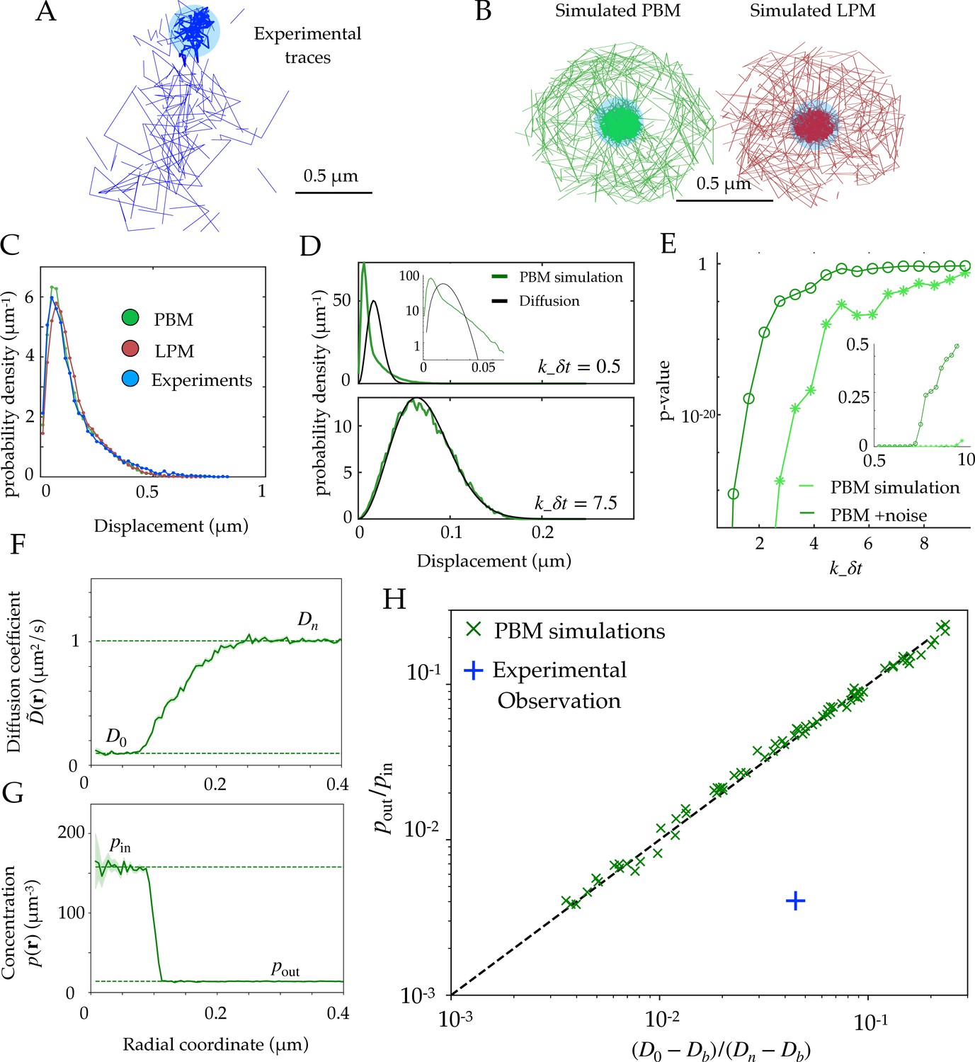
Diffusion properties and effective free energy.

(A) Example of experimental tracking of Rad52 molecules visiting a double-strand break (DSB) focus. Different connected traces correspond to distinct Rad52 molecules. (B) Example trajectory of a particle visiting the focus from simulations in the PBM (left) and LPM (right). The simulated trajectories are visually similar to the data in B. (C) Displacement histogram (jump sizes) for the PBM, LPM and experiments, for an interval $δ = 20$ ms. D. Displacement histogram for the PBM for small values of $k_{-} d t$ (top) and high values (bottom). Here we varied the interval from $δ t = 1$ ms (top) to $δ t = 15$ ms (bottom). (E) Hypothesis testing using a two sided KS-test, comparing the displacement histogram of a free diffusion process (black line in D) and the displacement histogram of diffusion inside the focus (green line in D). Parameters are the same as in (D) $δ t$ was varied from 1 to 25 ms. (F) Effective diffusion coefficient as a function of distance to the focus center $r$ , estimated from simulations of the PBM calculating $\tilde{D} = ⟨ δ r^{2} ⟩ / (2 d δ t)$ in each radial segment. (G) Particle density $p (r)$ as a function of $r$ , estimated from simulations of the PBM. Error bars are standard errors on the mean. (H) Relation between the ratio $(D_{0} - D_{b}) / (D_{n} - D_{b})$ versus the ratio of densities inside and outside the focus (From Equation 11), both estimated from simulations of the PBM (green crosses), compared to the identity prediction (Equation 12, black line). Blue cross shows the experimental observation for Rad52 in DSB loci (see text related to Figure 7 and Table S1 in Miné-Hattab et al., 2021). Parameter values as in Table 1 except: $r_{n} = 1 μ m$ for B; $A = 2.5 k_{B} T$ for B-C; $r_{n} = 0.3 μ m$ , $r_{f} = 0.15 μ m$ and $D_{n} = 0.5 μ m^{2} / s$ for D-E, $κ = 300 μ m / s$ for D, $r_{n} = 0.75 μ m$ for F-H. In H we varied $κ = 1$ – $400 μ m / s$ , $k_{-} = 1$ – $1, 500$ s-1, and $ρ = 2.4$ – $4.8 \cdot 10^{4} μ m$ . See Figure 2—source data 1.

Figure 2—source data 1 Compressed ZIP file containing all the data plotted in the panels of Figure 2 as CSV and TXT files.: https://cdn.elifesciences.org/articles/69181/elife-69181-fig2-data1-v2.zip
Download elife-69181-fig2-data1-v2.zip

Figure 2—figure supplement 1

Download asset Open asset

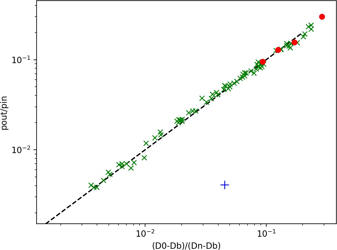
Effect of crowding.

Same as 2 H., but with added red points corresponding to replacing 20 % (leftmost), 40%, 60%, and 80 % (rightmost) of the binding sites by inert, totally reflecting spheres to simulate crowding. While crowding should decrease the measured D₀, in practice the effect is negligible.

Figure 3 with 1 supplement

Download asset Open asset

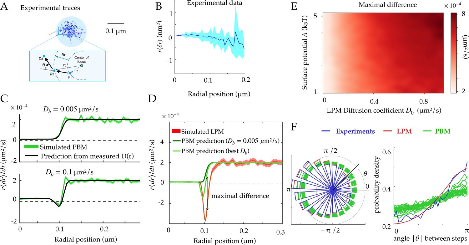
Radial and angular dynamics.

(A) Experimental trace of a single Rad52 in a DSB focus (Miné-Hattab et al., 2021). The inset shows the definition of the radial movement $δ r$ . Here, concentric circles are shown to define the radius relative to the focus center, where a particle moves a specific distance away from the center of the focus, as well as the angle $θ$ between consecutive displacements. (B) Data extracted from experiments (Miné-Hattab et al., 2021) to estimate the average radial displacement of the tracked particle multiplied by the radius. Here and throughout the x-axis represents the radial position at the beginning of the timestep. Error bars are standard errors on the mean. (C) Simulations showing the radial displacements in the PBM with slowly (top) and rapidly (bottom) moving binding sites. Black lines are predictions based on the measurement of $\tilde{D}$ (Equation 12). Error bars are standard deviations on the mean. (D) Radial displacement from simulations of the LPM. Light-green line shows the (wrong) prediction made while assuming the PBM, using the measurement of the effective diffusion coefficient $\tilde{D} (r)$ (Equation 13). We call the discrepancy between data and the PBM prediction the ‘‘Maximal positive difference.’’ Error bars are standard errors on the mean. (E) Heatmap showing the maximal positive difference in LPM simulations as a function of D₀ and $A$ . (F) Distribution of angles (represented radially on the left, and linearly on the right) between the displacements of consecutive steps of length $δ t$ , from experiments and simulations. Multiple curves for the PBM correspond to different parameter choices corresponding to the points of Figure 2H. Parameter values as in Table 1, except $r_{n} = 1 μ$ m for F. For F parameters are varied with $κ = 100$ – $300 μ$ m/s, $k_{-} = 500$ – $1, 500$ s $^{- 1}$ , $r_{f} = 0.1$ – $0.14 μ$ m. See Figure 3—source data 1 and Figure 3—source data 2.

Figure 3—source data 1 Compressed ZIP file containing all the data plotted in the panels of Figure 3 as CSV files.: https://cdn.elifesciences.org/articles/69181/elife-69181-fig3-data1-v2.zip
Download elife-69181-fig3-data1-v2.zip
Figure 3—source data 2 Compressed ZIP file containing all the data plotted in Figure 3—figure supplement 1 as CSV files.: https://cdn.elifesciences.org/articles/69181/elife-69181-fig3-data2-v2.zip
Download elife-69181-fig3-data2-v2.zip

Figure 3—figure supplement 1

Download asset Open asset

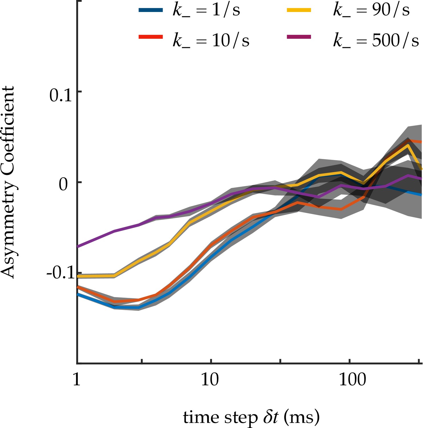
Asymmetry coefficient for an infinite PBM focus.

Asymmetry coefficient (following the definition of Izeddin et al., 2014), for an infinite focus, simulated with the PBM, as a function of the time step $δ t$ . Asymmetry is due to molecules reflecting off binding sites, causing more consecutive displacements to have 180 degree angles. The faster the binding and unbinding relative to the time step $δ t$ , the closer to mean-field limit of standard diffusion, and the more symmetric the angle distribution. $k_{+}$ is changed alongside $k_{-}$ to keep p_u constant. The asymmetry coefficient is defined as $\log_{2} [P (| θ | < π / 6) / P (| θ | > 5 π / 6)]$ , where $- π < θ < π$ . Standard deviation is obtained from four independent runs of 1000 s.

Figure 4

Download asset Open asset

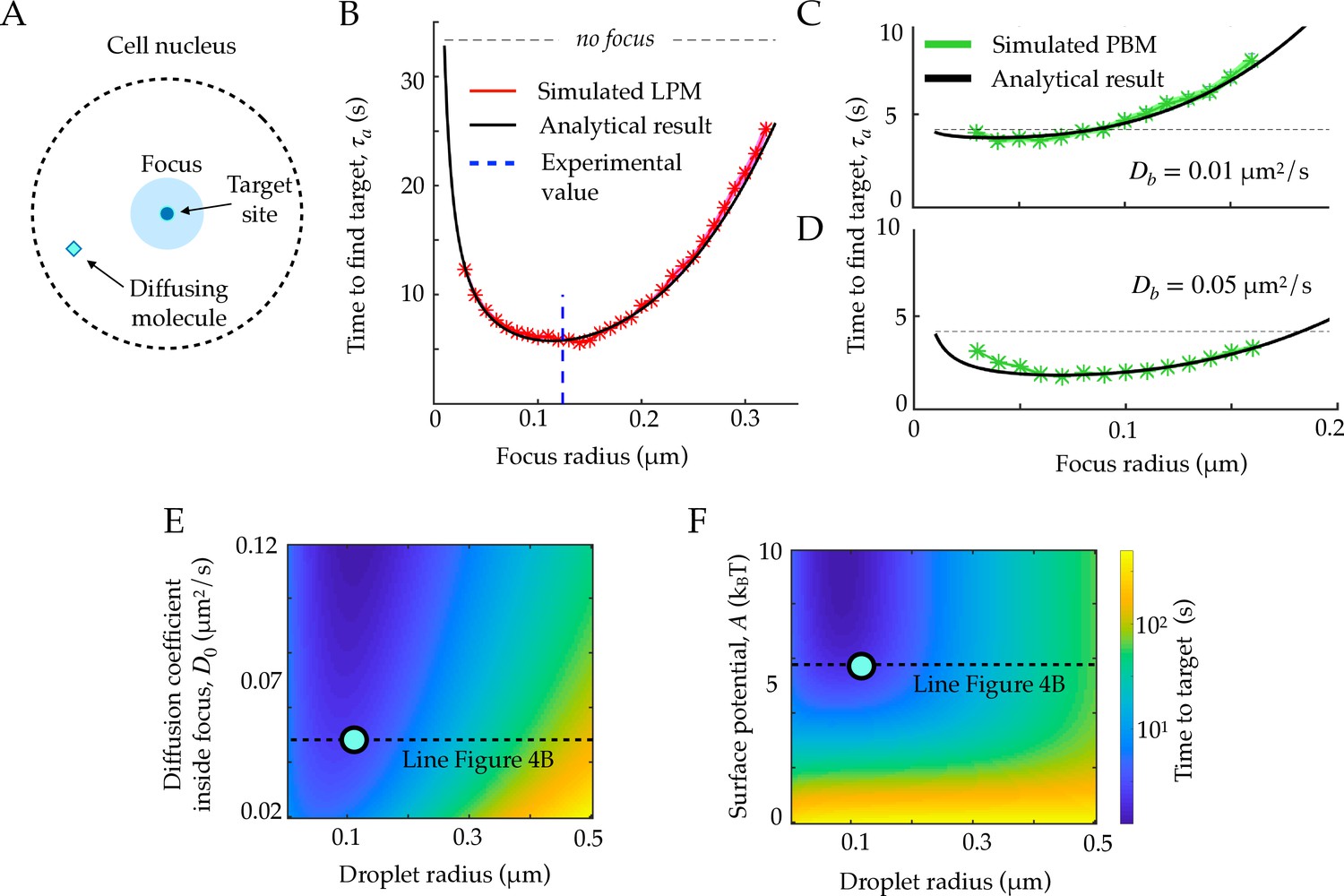
First passage times to a target site inside the focus.

A. Schematic figure showing the setup of the tracked molecule and the effective target. B. Time to reach the specific target in simulations for the LPM. Black curve shows the predicted result from the analytical derivation (Equation 15). Here we use parameters: $A = - 5.5 k_{B} T$ , $D_{0} = 0.05 μ^{2} / s$ , $r_{n} = 1.0 μ m$ , $D_{n} = 0.8 μ^{2} / s$ . C. Same as B, but for the PBM. Same parameters as in B, but with $D_{0} = D_{n} \cdot e^{U (r) / k_{B} T}$ . D. Heatmap showing the expected search time as a function of the droplet size (x-axis) and the focus diffusion coefficient (y-axis) (Equation 15). Green point corresponds to experimental observations. E. Heatmap showing the expected search time as a function of the droplet size (x-axis) and the height of the surface potential (y-axis) (Equation 15). Green point corresponds to experimental observations. Parameter values as in Table 1, except $b = 2, 000 μ m^{- 1}$ , $D_{0} = 0.04 μ m^{2} / s$ , $A = 5.5 k_{B} T$ for B, E, and F, $κ = 50 μ m^{2} / s$ , $k_{-} = 100$ s $^{- 1}$ , $ρ = 2.4 \cdot 10^{4} μ m^{- 3}$ for C-D. See Figure 4—source data 1.

Figure 4—source data 1 Compressed ZIP file containing all the data plotted in the panels of Figure 4 as CSV files.: https://cdn.elifesciences.org/articles/69181/elife-69181-fig4-data1-v2.zip
Download elife-69181-fig4-data1-v2.zip

Tables

Table 1

Parameters used in this study with their typical values, and the ranges we have considered.

Experimental values are from Miné-Hattab et al., 2021 (see Materials and Methods for details on estimating diffusion coefficients and free energy differences). D₀ and $A$ are model parameters in the LPM, but also effective observables in the PBM. The diffusivity of binding sites is taken to be that of Rfa1 molecules in the focus, which bind to single-stranded DNA in repair foci, and are thus believe to follow the diffusion of the chromatin (Miné-Hattab et al., 2021). The number $N$ of binding site is related to their density $ρ$ inside the focus through $N = (4 / 3) π ρ r_{f}^{3}$ .

Variable	Model	Description	Value	Range	Exp. value	Units
r_f	both	radius of focus	100	50–200		$nm$
r_n	both	radius of nucleus	500	300–1000		$nm$
$D_{n}$	both	Diffusion coefficient in nucleus	1.0	0.5–2.0	1.08	$μ m^{2} / s$
$σ$	both	Experimental noise level	30	30	30	$nm$
D₀	LPM	Diffusion coefficient inside droplet	0.05	0.01–0.5	0.032	$μ m^{2} / s$
$A$	LPM	Surface potential	5.0	0–10	5.5	$k_{B} T$
$b$	LPM	Steepness in potential	1,000	500–10000		$μ m^{- 1}$
$ρ$	PBM	Density of binding sites inside focus	$4.8 \cdot 10^{4}$	$1 \cdot 10^{3}$ - $8.4 \cdot 10^{4}$		$μ m^{- 3}$
$D_{b}$	PBM	Diffusion coefficient of binding sites	0.005	0-0.1	0.005	$μ m^{2} s^{- 1}$
r_b	PBM	Radius of binding sites	10	5-20		nm
$k_{-}$	PBM	Unbinding rate	500	10-10,000		$s^{- 1}$
$κ$	PBM	Absorption parameter	100	0-1000		$μ m / s$