Diverse mating phenotypes impact the spread of wtf meiotic drivers in Schizosaccharomyces pombe
- Stowers Institute for Medical Research, United States
- Kenyon College, United States
- Department of Molecular and Integrative Physiology, University of Kansas Medical Center, United States
Abstract
Meiotic drivers are genetic elements that break Mendel’s law of segregation to be transmitted into more than half of the offspring produced by a heterozygote. The success of a driver relies on outcrossing (mating between individuals from distinct lineages) because drivers gain their advantage in heterozygotes. It is, therefore, curious that Schizosaccharomyces pombe, a species reported to rarely outcross, harbors many meiotic drivers. To address this paradox, we measured mating phenotypes in S. pombe natural isolates. We found that the propensity for cells from distinct clonal lineages to mate varies between natural isolates and can be affected both by cell density and by the available sexual partners. Additionally, we found that the observed levels of preferential mating between cells from the same clonal lineage can slow, but not prevent, the spread of a wtf meiotic driver in the absence of additional fitness costs linked to the driver. These analyses reveal parameters critical to understanding the evolution of S. pombe and help explain the success of meiotic drivers in this species.
Editor's evaluation
Meiotic drivers are selfish elements that distort segregation to be over-represented in offspring of heterozygotes. Multiple meiotic drive elements are known in the yeast Schizosaccharomyces pombe, S. pombe, which can seem puzzling as this fungus has long been thought to undergo little outcrossing. This manuscript reports theoretical and experimental analyses suggesting that the outcrossing rate can be high enough in this species to explain the spread of multiple meiotic drive elements. The findings support the emerging view that homothallic fungi can undergo quite high rates of outcrossing, which is also in agreement with evolutionary considerations on the evolution of mating types. This study can thus be of high relevance for scientists studying meiotic drivers and/or mating systems and their evolution.
https://doi.org/10.7554/eLife.70812.sa0eLife digest
The fission yeast, Schizosaccharomyces pombe, is a haploid organism, meaning it has a single copy of each of its genes. S. pombe cells generally carry one copy of each chromosome and can reproduce clonally by duplicating these chromosomes and then dividing into two cells. However, when the yeast are starving, they can reproduce sexually. This involves two cells mating by fusing together to create a ‘diploid zygote’, which contains two copies of each gene. The zygote then undergoes ‘meiosis’, a special type of cell division in which the zygote first duplicates its genome and then divides twice. This results in four haploid spores which are analogous to sperm and eggs in humans that each contain one copy of the genome. The spores will grow and divide normally when conditions improve.
The genes carried by each of the haploid spores depend on the cells that formed the zygote. If the two ‘parent’ yeast had the same version or ‘allele’ of a gene, all four spores will have it in their genome. However, if the two parents have different alleles, only 50% of the offspring will carry each version. Although this is usually the case, there are certain alleles, called meiotic drivers, that are transmitted to all offspring even in situations where it is only carried by one parent. Meiotic drivers can be found in many organisms, including mammals, but their behavior is easiest to study in yeast.
Meiotic drivers known as killers achieve this by disposing of any ‘sister’ spores that do not inherit the same allele of this gene. This ‘killing’ can only happen when only one of the ‘parents’ carries the driver. This scenario is thought to rarely occur in species that inbreed, as inbreeding leads to both gene copies being the same. However, this does not appear to be the case for S. pombe, which contain a whole family of killer meiotic drivers, the wtf genes, despite also being reported to mainly inbreed.
To investigate this contradiction, López Hernández et al. isolated several genetically distinct populations of S.pombe. These isolates were grown together to determine how often the each one would outcross (mate with an individual from a different population) or inbreed. The results found that levels of inbreeding varied between isolates.
Next, López Hernández et al. used mathematical modelling and experimental evolution analyses to study how wtf drivers spread amongst these populations. This revealed that wtf genes spread faster in populations with more outcrossing. In some instances, the wtf driver was linked to a gene that could harm the population. In these cases, López Hernández et al. found than inbreeding could purge these drivers and stop them from spreading the dangerous alleles through the population.
López Hernández et al. establish a simple experimental system to model driver evolution and experimentally demonstrate how key parameters, such as outcrossing rates, affect the spread of these genes. Understanding how meiotic drivers spread is important, as these systems could potentially be used to modify populations important to humans, such as crops or disease vectors.
Introduction
Mating behaviors have long been a focus of art, literature, and formal scientific inquiry. This interest stems, in part, from the remarkable importance of mate choice on the evolution of species. Outcrossing and inbreeding represent distinct mating strategies that both have potential evolutionary benefits and costs (Glémin et al., 2019; Muller, 1932; Otto and Lenormand, 2002). For example, outcrossing (mating between individuals from distinct lineages) can be beneficial because it can help purge deleterious alleles from a line of descent, but it can also be costly as it can promote the spread of selfish genes (Burt and Trivers, 1998; Crow, 1988; Hurst and Werren, 2001; McDonald et al., 2016; Zeyl et al., 1996).
Meiotic drivers represent one type of selfish genetic element that relies on outcrossing to persist and spread in a population (Lindholm et al., 2016; Sandler and Novitski, 1957). These loci can manipulate the process of gametogenesis to bias their own transmission into gametes at the expense of the rest of the genome (Burt and Trivers, 2006). Meiotic drivers are often considered selfish or parasitic genes because they generally offer no fitness benefits to their hosts and are instead often deleterious or linked to deleterious alleles (Dyer et al., 2007; Higgins et al., 2018; Klein et al., 1984; Rick, 1966; Schimenti et al., 2005; Taylor et al., 1999; Wilkinson and Fry, 2001). As inbreeding is thought to inhibit the spread of selfish genes like drivers, drivers are predicted to be unsuccessful in species that rarely outcross (Burt and Trivers, 1998; Hurst and Werren, 2001). This assumption appears to be challenged in several fungal species, including the fission yeast Schizosaccharomyces pombe (Grognet et al., 2014; Hammond et al., 2012; Svedberg et al., 2021; van der Gaag et al., 2000; Vogan et al., 2021).
Generally, S. pombe cells grow as haploids and their mating (fusion of two haploids of opposite mating type) generates diploid zygotes that can then undergo meiosis to generate haploid progeny known as spores (Figure 1—figure supplement 1A). Mating in S. pombe is widely thought to preferentially occur between daughter cells clonally derived from a common progenitor via a recent mitotic division, which we refer to as ‘same-clone mating’ (Figure 1—figure supplement 1B; Egel, 1977; Gutz and Doe, 1975; Miyata and Miyata, 1981; Billiard et al., 2012; Perrin, 2011). The support for this idea is described below. Despite this notion that S. pombe cells preferentially undergo same-clone mating (leading to inbreeding), S. pombe isolates host multiple meiotic drivers (Bravo Núñez et al., 2020b; Eickbush et al., 2019; Farlow et al., 2015; Hu et al., 2017; Nuckolls et al., 2017; Zanders et al., 2014).
In the wild, a minority of S. pombe strains are heterothallic, meaning they have a fixed mating type (h+ or h-; Gutz and Doe, 1975; Nieuwenhuis and Immler, 2016; Schlake and Gutz, 1993). Heterothallic S. pombe strains must mate with non-clonally related cells of the opposite mating type to complete sexual reproduction (Egel, 1977; Gutz and Doe, 1975; Leupold, 1949; Miyata and Miyata, 1981; Nieuwenhuis and Immler, 2016; Osterwalder, 1924; Schlake and Gutz, 1993). However, most isolates of S. pombe are homothallic, that is, they can switch between the two mating types (h+ and h-) during clonal expansion via mitosis (Figure 1—figure supplement 1B; Egel and Eie, 1987; Gutz and Doe, 1975; Klar, 1990; Nieuwenhuis et al., 2018; Singh and Klar, 2003). Homothallism in S. pombe enables mating to occur between cells clonally derived from the same progenitor via mitosis (Billiard et al., 2012). Mating can even occur between two cells produced by a single mitotic cell division (Egel, 1977; Gutz and Doe, 1975; Miyata and Miyata, 1981).
It is often assumed that homothallic fungi, like S. pombe, do not generally mate with non-clonally related cells. It is important to note, however, that homothallism in fungi does not inherently lead to mating between clonally related cells (Giraud et al., 2008). Under some conditions, such as when gametes are dispersed and finding a mate is costly, homothallism can be a beneficial strategy for outcrossing species as it ensures gamete compatibility (Billiard et al., 2012). In addition, population genetic analyses of one homothallic fungus, Sclerotinia sclerotiorum, support that homothallism is compatible with frequent outcrossing (Attanayake et al., 2014).
Very little is known about the ecology of S. pombe in the wild, including how often S. pombe cells outcross (Jeffares, 2018). In the lab, the mating propensities of S. pombe have mostly been investigated in derivatives of a strain first isolated from French wine in 1921 (Osterwalder, 1924). In this work, we will refer to derivatives of this isolate as ‘Sp’. Distinct homothallic Sp strains can be induced to mate in the lab (i.e., outcrossed), but such crosses are significantly more challenging to execute than crosses between heterothallic isolates. The relative difficulty associated with outcrossing homothallic strains has been attributed to preferential same-clone mating (Ekwall and Thon, 2017; Forsburg and Rhind, 2006). Microscopy experiments have supported the idea that homothallic Sp haploids tend to undergo same-clone mating (Bendezú and Martin, 2013; Egel, 1977; Leupold, 1949; Miyata and Miyata, 1981). However, the precise level of same-clone mating when homothallic S. pombe cells are among nonclonal sexual partners has not, to our knowledge, been formally reported for any isolate.
Population genetic analyses have provided additional support for the notion that S. pombe inbreeds. There are two major S. pombe lineages that diverged between 2300 and 78,000 years ago (Tao et al., 2019; Tusso et al., 2019). Much of the sampled variation within the species represents different admixed hybrids of those two ancestral lineages resulting from an estimated 20–60 outcrossing events (Tusso et al., 2019). This low outcrossing rate could result from limited opportunities to outcross, preferential same-clone mating, or a combination of the two. It is important to note, however, that the outcrossing rate estimates in S. pombe are likely low as pervasive meiotic drive and decreased recombination in heterozygotes suppress the genetic signatures that are used to infer outcrossing (Bravo Núñez et al., 2020b; Hu et al., 2017; Nuckolls et al., 2017; Zanders et al., 2014).
Accounting for all these factors to generate a more accurate S. pombe outcrossing rate from population genetic data is currently an insurmountable obstacle for several reasons. First, the landscape of meiotic drivers and their suppressors is complex in that more than four drivers and more than eight suppressors of drive could be present in a given heterozygote produced by outcrossing (Eickbush et al., 2019; Bravo Núñez et al., 2020a). Predicting how those factors will affect allele transmission is well beyond the capabilities of current population genetic models, even if the epistatic relationships within the drive systems were understood, which they currently are not. In addition to the drivers, S. pombe isolates contain an array of chromosomal rearrangements and other unknown barriers to recombination (Avelar et al., 2013; Brown et al., 2011; Jeffares et al., 2017; Tusso et al., 2019; Zanders et al., 2014). Importantly, recombination rates are also inextricably linked to the complex drive landscape because the presence of drivers also affects the recombination rate within viable offspring, independent of chromosomal rearrangements (Bravo Núñez et al., 2020b).
Given those limitations, the current laboratory knowledge and outcrossing rate estimates suggest that drivers would infrequently have the opportunity to act in S. pombe (Egel, 1977; Ekwall and Thon, 2017; Forsburg and Rhind, 2006; Gutz and Doe, 1975; Miyata and Miyata, 1981; Tusso et al., 2019). In fact, the notion that S. pombe infrequently outcrosses has even been used to challenge the idea that S. pombe meiotic drivers are truly selfish genes that persist due to meiotic drive (Sweigart et al., 2019). Nonetheless, the S. pombe genome houses numerous meiotic drive genes from the wtf gene family (Bravo Núñez et al., 2018; Bravo Núñez et al., 2020a; Eickbush et al., 2019; Hu et al., 2017; Nuckolls et al., 2017).
The wtf drivers destroy the meiotic products (spores) that do not inherit the driver from a heterozygote. Each wtf drive gene encodes both a Wtfpoison and a Wtfantidote protein that, together, execute targeted killing of the spores that do not inherit the wtf driver (Hu et al., 2017; Nuckolls et al., 2017). In the characterized wtf4 driver, the Wtf4poison protein assembles into toxic protein aggregates that are packaged into all developing spores. The Wtf4antidote protein co-assembles with Wtf4poison only in the spores that inherit wtf4 and likely neutralizes the poison by promoting its trafficking to the vacuole (Nuckolls et al., 2020). Spore killing by wtf drivers leads to the loss of about half of the spores and almost exclusive transmission (>90%) of the wtf driver from a heterozygote (Hu et al., 2017; Nuckolls et al., 2017). Despite their heavy costs to the fitness of heterozygotes, the drivers are successful in that all assayed S. pombe isolates contain multiple wtf drivers (4–14 drivers; Bravo Núñez et al., 2020a; Eickbush et al., 2019; Hu et al., 2017). In addition to those drivers, the S. pombe isolates also contain between 8 and 17 suppressors of drive that encode only a Wtfantidote protein.
In this work, we exploited the tractability of S. pombe to better understand how mating phenotypes, particularly inbreeding propensity, could affect the spread of a meiotic driver in this species. Despite limited genetic diversity among isolates, we observed natural variation in inbreeding propensity and other mating phenotypes. Some natural isolates preferentially undergo same-clone mating in the presence of a potential outcrossing partner, whereas others mate more randomly. Additionally, we found that the level of same-clone mating can be altered by cell density and affected by the available sexual partners. This is important as it highlights that our measured values in the lab are not meant to indicate precise levels of outcrossing that would occur under unknown natural conditions.
To explore the effects that varying mating phenotypes could have on the spread of a wtf driver in a population, we used both mathematical modeling and an experimental evolution approach. We found that, while the spread of a wtf driver could be slowed by the observed levels of same-clone mating, the driver could still spread in the absence of linked deleterious traits. We incorporated our observations into a model in which rapid wtf gene evolution and occasional outcrossing facilitate the maintenance of wtf drivers. More broadly, this study illustrates how the success of drive systems is impacted by mating phenotypes.
Results
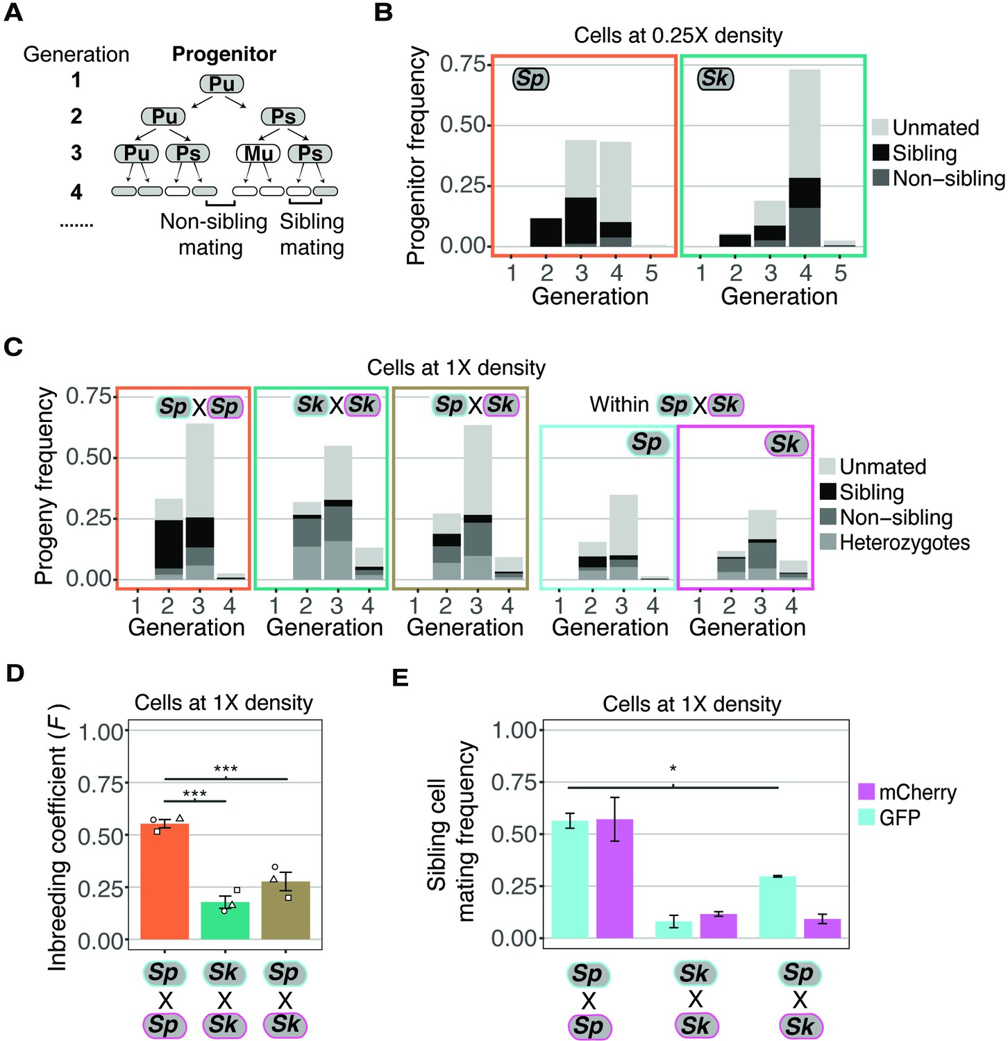
Same-clone mating propensity differs among S. pombe natural isolates
To quantify mating propensities of homothallic S. pombe strains in the presence of other potential homothallic sexual partners, we first generated fluorescently tagged strains to easily observe mating via microscopy (Figure 1A). We marked strains with either GFP or mCherry (both constitutively expressed and integrated at the ura4 locus). We then mixed equal proportions of GFP-expressing and mCherry-expressing haploid cells and plated them on a medium (SPA) that induces one round of mating and meiosis. We imaged the cells immediately after plating to measure the starting frequency of both parent types. We then imaged again 24–48 hr later when many cells in the population had mated to either form zygotes or fully developed spores. We inferred the genotypes (homozygous or heterozygous) of each zygote and ascus (spore sac) based on their fluorescence (Figure 1A). Homozygotes were produced by mating of two cells carrying the same fluorophore, while heterozygotes were produced by mating between a GFP-labeled and an mCherry-labeled cell (Figure 1B and C). Finally, we calculated the inbreeding coefficient (F) by comparing the observed frequency of heterozygotes to the frequency expected if mating was random (F = 1–observed heterozygotes/expected heterozygotes; Figure 1A). Exclusive mating between cells with the same fluorophore, random mating, and exclusive mating between cells with different fluorophores would yield coefficients of 1, 0, and –1, respectively (Hartl and Clark, 2007). This assay occurs in a specific laboratory context, so the conditions differ from those in the wild. Importantly, however, we assay all strains under the same conditions, so the assay is sufficient to explore possible variation in mating phenotypes between different isolates of S. pombe.
Figure 1 with 4 supplements see all

Inbreeding coefficients vary between homothallic isolates of Schizosaccharomyces pombe.
(A) Experimental strategy to quantify mating patterns between mixed homothallic isolates. GFP (cyan)- and mCherry (magenta)-expressing cells were mixed and placed on SPA medium that induces mating and meiosis. An agar punch from this plate was imaged to assess the initial frequencies of each haploid strain. After incubation at 25°C for at least 24 hr, another punch was imaged to determine the number of homozygous and heterozygous zygotes/asci based on their fluorescence. The inbreeding coefficient (F) was calculated using the formula shown. (B and C) Representative images of the mating in Sp (B) and Sk (C) isolates after 24 hr. Filled arrowheads highlight examples of homozygous asci whereas open arrowheads highlight heterozygous asci. A few additional zygotes are also outlined with dotted lines in the images. Scale bars represent 10 µm. (D) Inbreeding coefficient of homothallic natural isolates and complementary heterothallic (h+,h- mCherry and h+,h- GFP) Sp lab strains. At least three biological replicates per isolate are shown (open shapes). (E) Mating efficiency of the isolates shown in (D) (%) ± standard error from three biological replicates of each natural isolate.
-
Figure 1—source data 1
Schizosaccharomyces pombe natural isolates.
List of S. pombe natural isolates reported by Tusso et al., 2019. Those selected to measure inbreeding coefficients using microscopy are highlighted and observations for these from other studies are reported (Jeffares et al., 2015; Nieuwenhuis et al., 2018).
- https://cdn.elifesciences.org/articles/70812/elife-70812-fig1-data1-v2.xlsx
In homothallic cells of the common lab isolate, Sp, we measured an average inbreeding coefficient of 0.57 using our microscopy assay (Figure 1B and D). As a control, we also assayed a mixed heterothallic population containing roughly equal amounts of GFP-expressing and mCherry-expressing cells of both mating types. We expected this control population to exhibit random mating between GFP- and mCherry-expressing cells, as heterothallic cells cannot undergo same-clone mating. We did observe random mating of this mixed heterothallic population (F = −0.05), which helps validate our assay (Figure 1D). To further validate our microscopy results, we also assayed Sp cells using an orthogonal approach employing traditional genetic markers. For this analysis, we mixed haploid cells on supplemented SPA medium (SPAS) to induce them to mate and undergo meiosis. We then manually genotyped the progeny and used the fraction of recombinant progeny to calculate inbreeding coefficients (Figure 1—figure supplement 2A). The average inbreeding coefficients measured using the genetic assay were very similar to the values we measured using the microscopy assay (0.49 for homothallic Sp cells; Figure 1—figure supplement 2B). Together, our results confirm and quantify previous observations of non-random mating in homothallic Sp cells (Bendezú and Martin, 2013; Egel, 1977). In addition, we demonstrate that our fluorescence assay provides a powerful tool to quantify mating events.
We next extended our analyses to other S. pombe natural isolates collected from the wild. We assayed six additional isolates, FY29043, FY29022, FY28981, FY28974, FY29044, and Schizosaccharomyces kambucha (Sk), using our fluorescence microscopy assay. We chose these isolates because they each contain different fractions of the two inferred ancestral S. pombe lineages (Tusso et al., 2019). In addition, the strains we chose are homothallic, sporulated well, were non-clumping, and we were able to transform them with the GFP and mCherry markers described above (Figure 1—source data 1, Figure 1—figure supplement 3; Jeffares et al., 2015). We found that the measured inbreeding coefficients varied significantly between the different natural isolates (Figure 1D). The phenotype of FY29043 was similar to Sp, but other S. pombe isolates, including Sk, mated more randomly (Figure 1D). We also observed variation in mating efficiency ranging from 10% of cells mating in FY28981 to 50% of cells mating in Sk (Figure 1E).
Given that S. pombe cells are immobile, we thought that cell density could affect their propensity to undergo same-clone mating. To test this, we compared the inbreeding coefficients of both homothallic Sp and Sk isolates at three different starting cell densities: our standard mating density (1×), high density (10×), and low density (0.1×). Because crowding prevented us from assaying high-density cells using our microscopy approach, we used the genetic assay for each condition. We found that inbreeding coefficients were higher in both Sp and Sk isolates when cell densities were lower (Figure 1—figure supplement 2C and D). This is likely because cells plated at low density tended to be physically distant from potential sexual partners that were not part of the same clonally growing patch of cells (Figure 1—figure supplement 4). However, a control population consisting of mixed heterothallic Sp cells (h+ and h- cells of two different genotypes mixed in equal proportions) that cannot mate within a clonal patch of cells showed near random mating between the two genotypes at all cell densities assayed (Figure 1—figure supplement 2C). Overall, these experiments demonstrate that inbreeding coefficients vary within S. pombe homothallic isolates and can be affected by cell density.
Additional phenotypes associated with reduced inbreeding coefficients in Sk
We next used time-lapse imaging to explore the origins of the different inbreeding coefficients, focusing on the Sp and Sk isolates. Previous work claimed that Sk cells have reduced mating-type switching efficiency, based on levels of the DNA break (double-strand break site [DSB]) that initiates switching (Singh and Klar, 2002). A mutation at the mat-M imprint site was proposed to be responsible for the reduced level of DSBs (Singh and Klar, 2003).
We reasoned that less mating-type switching could lead to less same-clone mating, as a small population of cells clonally derived from the same progenitor via mitosis would be less likely to contain cells of compatible mating types. This would promote cells mating outside their clonal lineage. One can see evidence consistent with this phenomenon in our experiments varying the cell density of homothallic Sp cells (Figure 1—figure supplement 2C-D). Specifically, we observed more random mating when cells were at higher density, which likely results from more opportunity for cells to mate outside their clonal lineage. We aspired to directly compare mating type switching rates between Sp and Sk cells, although such direct assays have not, to our knowledge, been done in any strain background. We attempted to develop a direct assay using previously described cytological reporters of mating type. The reporters have been used to assay ratios of h + and h- cells in a population (Jakočiūnas et al., 2013, Maki et al., 2018), but we found they were not well-suited for following switching events live in time-lapse imaging in our hands (Figure 2—figure supplement 1A).
Because of this, we decided to further explore the possible differences in mating-type switching frequencies indirectly using time-lapse assays, similar to those used to originally determine the patterns of mating-type switching in Sp (Miyata and Miyata, 1981). As in the classic study of Miyata and Miyata, 1981, we used the first mating event as an imperfect proxy for when cells were capable of mating (i.e., they had a partner of the opposite mating type). For these assays, we tracked the fate of individual homothallic founder cells plated on SPA at low density (0.25× to our standard mating density used above) to quantify how many mitotic generations occurred prior to the first mating event. When the first mating event occurred, we recorded the proportion of the cells present that mated (prior to the appearance of cells from next mitotic generation). We also recorded the relationships between the cells that did mate (Figure 2A). Specifically, we scored whether the mated cells were the product of a single mitotic division. Historically, these have been called ‘sister cells’ in the S. pombe mating literature, although we use the term ‘sibling cells’ to be gender neutral (e.g., Miyata and Miyata, 1981). We did not consider cells that were born in mitotic generations past the one in which mating first occurred (Figure 2A). For example, if cells within a given lineage first mated at generation 3, we scored the relationships between those mated cells and recorded how many unmated cells remained at the end of generation 3 (even if descendants of the unmated cells eventually mated). We then did not consider that lineage any further, so lineages in which cells first mated at generation 2 are not represented in the generation 3 data.
Figure 2 with 7 supplements see all
Variation between mating behaviors in Sp and Sk cells.
(A) Schematic showing cell divisions, switching, and mate choice in Sp. Mitotic generations are shown on the left. Cells are either h+ (P) or h- (M) and their status is switchable (s) or unswitchable (u). (B) Division and mating phenotypes of wildtype Sp and Sk cells plated at low cell density (0.25×) on SPA plates. Single founder cells and their descendants were monitored through time-lapse imaging. Mating patterns were categorized until the end of the generation in which the first mating event occurred. The data presented were pooled from two independent time-lapses in which over 400 founder cells were tracked. (C) Division and mating phenotypes of fluorescently labeled Sp and Sk cells plated at standard (1×) density on SPA plates. Individual cells were monitored until the population reached a typical mating efficiency for the specific cross and the mate choice of their progeny and the mitotic generation of those events was classified. The cells labeled with GFP are indicated with a cyan line around the cell whereas the mCherry-labeled cells are outlined in magenta. Pooled data from two independent experiments are presented, with 286 cells scored from each experiment. In the cross of Sp (GFP) and Sk (mCherry), we present an additional plot (far right) in which the fate of each founder is separated by isolate. (D) Inbreeding coefficient calculated from still images of cells plated at 1× density on SPA. *** indicates p-value < 0.005, multiple t-test, Bonferroni corrected. At least three biological replicates per isolate are shown (open shapes). (E) Breakdown of sibling cell mating by fluorophore in the indicated crosses from C. * indicates p-value = 0.04, one-tailed t-test comparing isogenic and mixed Sp cells from two videos.
Classic work characterizing mating-type switching patterns in Sp found that one in a group of four clonally derived cells will have the opposite mating type relative to the other three cells. A newly switched cell will be compatible to mate with close relatives, most typically its sibling cell (Figure 2A; Miyata and Miyata, 1981). Under the same switching model, a smaller portion of cells derived from a single division could be of opposite mating types and thus sexually compatible. For example, if one considers switchable cells (e.g., Ps in Figure 2A), they must divide only once to generate a pair of mating-competent cells. In Sp cells, we observed mating among the clonal descendants of some progenitor cells after a single mitotic division (i.e., at generation 2). By the third generation, we observed mating among the descendants of more than half of the progenitor cells. Almost all the observed mating events were between sibling cells (Figure 2A and B). These observations are consistent with published work assaying mating patterns within lineages of clonal Sp cells (Bendezú and Martin, 2013; Klar, 1990; Miyata and Miyata, 1981).
Sk cells plated at 0.25× density on SPA divided significantly more than Sp cells prior to the first mating (Wilcox rank sum test; p < 0.005 Figure 2B). Sk progenitor cells most frequently started mating at the fourth mitotic generation (Figure 2B). This phenotype is consistent with less mating-type switching as more generations would be required on average to produce a cell with the opposite mating type (Singh and Klar, 2002). In addition, many mating events were between non-sibling cells. This phenotype can also be explained indirectly by reduced mating-type switching. Specifically, after cells undergo several divisions, they generate non-linear cell clusters in which comparably more non-sibling cells are in close proximity (Figure 2—figure supplement 1A-B). This clustering could lead to more non-sibling mating than when cells are mating-competent after fewer divisions and the low number of cells are largely arranged linearly.
To better understand the differences between Sp and Sk, we compared the sequence of the mating-type locus in the two isolates as many distinct alleles have been identified (Nieuwenhuis et al., 2018). Consistent with previous work, we found that the mating-type regions of Sp and Sk are highly similar (Singh and Klar, 2002). However, using a previously published mate-pair sequencing dataset, we discovered an ~5 kb insertion of nested Tf transposon sequences in the Sk mating-type region (Eickbush et al., 2019). We confirmed the presence of the insertion using PCR (Figure 2—figure supplement 2A-B). We also found evidence consistent with the same insertion in FY28981, which also mates more randomly than Sp (Figure 2—figure supplement 2B, Figure 1D). We did not, however, formally test if the insertion affects mating phenotypes. Even if it does have an effect, it is insufficient to explain all the mating variation we observed as FY29044 mates randomly, yet it lacks the insertion (Figure 1D and Figure 2—figure supplement 2B).
To further explore the hypothesis that decreased mating-type switching efficiency in Sk could contribute to the mating differences we observed (Figure 2B), we carried out time-lapse analyses of cells, at our standard 1× cell mating density. We reasoned that at this density, any given cell is likely to have a cell of opposite mating type nearby, even if mating-type switching is infrequent. We again used mixed populations of GFP- and mCherry-expressing cells to facilitate the scoring of mating patterns (Figure 2C, Figure 2—video 1 supplement 1). We found that the Sp cells predominantly mated in the second and third mitotic generations and most mating events were between sibling cells (Figure 2C).
The mating behavior of Sk cells changed more dramatically between 0.25× density and the higher 1× density. Whereas Sk cells tended to first mate in the fourth generation at 0.25× density, at 1× density Sk cells, like Sp, generally mated in the second and third mitotic generations (Figure 2C, Figure 2—video 2 supplement 2). Additionally, we observed significantly reduced levels of mating between Sk sibling cells at 1× density relative to 0.25× (10% and 56%, respectively; Figure 2E and B). These phenotypes are consistent with reduced mating-type switching in Sk. Specifically, our data suggest that Sk cells do not need to undergo more divisions before they are competent to mate. Rather, the additional divisions that occurred at 0.25× density in Sk could have been necessary to produce a pair of cells with opposite mating types. At 1× density, additional divisions are not expected to be required as additional non-sibling compatible partners are available.
It is important to note, however, that our experiments combined with the previous work showing fewer switching-initiating DSBs in Sk (Singh and Klar, 2002), support, but do not conclusively demonstrate that mating-type switching occurs less frequently in Sk. In particular, our assays to understand switching frequencies use mating as a proxy for switching, which is not ideal. Therefore, reduced switching in Sk represents a promising model that remains to be tested. Still, our results conclusively demonstrate the key point that the mating phenotypes previously measured in Sp do not apply to all S. pombe isolates. Despite very little genetic diversity, S. pombe isolates maintain significant natural variation in key mating phenotypes (Jeffares et al., 2017).
Ascus variation
While assaying inbreeding cytologically, we noticed that the Sk natural isolate displayed tremendous diversity in ascus size and shape (Figure 1C, Figure 2—figure supplement 3A, Figure 2—video 2). This was due to high variability in the size of the mating projections, known as shmoos. Sk produced long shmoos only in response to cells of the opposite mating type and not as a response to nitrogen starvation alone (Figure 2—figure supplement 3B). The long Sk shmoos motivated us to quantify asci length across all the natural isolates described above. We found that most isolates generated zygotes or asci that were ~10–15 μm, similar to Sp. The majority of Sk zygotes and asci also fell within this range, but ~25% of Sk zygotes and asci were longer than 15 μm, with some exceeding 30 μm (Figure 2—figure supplement 3C). We also assayed zygote/ascus length in an additional natural isolate in which we were unable to quantify inbreeding due to a clumping phenotype (FY29033). This isolate also showed populations of long asci, like Sk (Figure 2—figure supplement 3C).
Additionally, we occasionally noticed a fused asci phenotype in Sk (Figure 2—figure supplement 3D). Time-lapse analyses of mating patterns, described above, revealed these fused asci can result from an occasional disconnect between mitotic cycles and the physical separation of cells (Figure 2—figure supplement 3E). This phenotype is reminiscent of adg1, adg2, adg3, and agn1 mutants in Sp that have defects in cell fission (Alonso-Nuñez et al., 2005; Gould and Simanis, 1997; Sipiczki, 2007). Although we observed this phenotype in all time-lapse experiments using Sk cells, the prevalence of this phenotype varied greatly between experiments. We rarely observed this phenotype in Sp cells. We did not analyze time-lapse images of the other natural isolates, where this phenotype is most easily observed, so it is unclear if this septation phenotype occurs in other natural isolates.
Mating phenotypes are affected by available mating partners
We next assayed if the mating preferences of S. pombe isolates Sp and Sk were invariable, or if they could be affected by the available mating partners due to mating incompatibilities (Seike et al., 2019b). To test this idea, we used both still and time-lapse imaging of cells mated at 1× density on SPA. For these experiments, we mixed fluorescently labeled Sp and Sk cells in equal frequencies.
We observed in experiments employing still images that the overall inbreeding coefficient of the mixed Sk/Sp population of cells was intermediate between single-isolate crosses and mixed crosses (Figure 2D). In time-lapse experiments, we observed that Sk cells maintained low levels of mating between sibling cells in the mixed Sk/Sp population (9.2% compared to 9.8% in a homogeneous population; Figure 2E). Among the Sp cells, mating between sibling cells decreased significantly from 56.8% to 29.7% in the mixed mating environment (Figure 2E; t-test, p = 0.04). Together, these results suggest that Sk cells can interfere with the ability of Sp cells to undergo same-clone mating. Although sibling cell mating preference changed, we did not observe a significant decrease in the mating efficiency of Sp cells in a mixed Sp/Sk population relative to a pure Sp population (Figure 2—figure supplement 4A). Instead, the mating efficiency in the mixed Sp/Sk population was intermediate of those observed in pure Sp and Sk populations, indicating these isolates do not affect each other’s ability to mate.
We were intrigued by the idea that long shmoos (mating projections) of Sk could contribute to its ability to disrupt Sp sibling mating. We were unable to address this idea directly. We did, however, find that Sk/Sp matings produce significantly longer zygotes/asci than either Sk/Sk or Sp/Sp matings (Figure 2—figure supplement 4B). This was true even when we compared Sk/Sp zygote/ascus length to the length of heterozygous Sk/Sk or heterozygous Sp/Sp zygotes/asci. While this result does not prove that long Sk shmoos disrupt Sp sibling mating, it does show that long shmoos tend to be used in these outcrossing events.
We next extended our analyses by assaying mating efficiency and inbreeding coefficients in all pairwise combinations of Sp, Sk, FY29043, and FY29044 using still images of mated cells. After adjusting for mating efficiencies and parental inbreeding coefficients (see Materials and methods), the phenotypes we observed in these crosses were mostly additive, in that they were intermediate to the pure parental strain phenotypes (Figure 2—figure supplement 5). The two exceptions were in the crosses between Sk and the isolates FY20943 and FY20944. Sk formed more Sk/Sk homozygotes than expected in the two crosses (one-tailed t-test, p = 0.043 and p = 0.038, respectively), suggesting that Sk cells may not be fully sexually compatible with FY20943 and FY20944 (Figure 2—figure supplement 5). However, the magnitude of the effect was small in both cases and the statistical significance is lost after Bonferroni correction for multiple testing. Overall, our observations indicate that mating phenotypes of a given isolate can be affected by different mating partners. Importantly, however, our results suggest mating incompatibilities are unlikely to have a major role in limiting outcrossing within S. pombe.
Population genetics modeling of the effect of inbreeding on a wtf meiotic driver
We next wanted to test how the observed range of inbreeding coefficients would affect the spread of a wtf driver in a population. To do this, we first used population genetic modeling. We used the meiotic drive model presented by J Crow, but we also introduced an inbreeding coefficient (Hartl and Clark, 2007; Crow, 1991) (see Materials and methods for a full description of the model). The model considers a population with two possible alleles at the queried locus and no genetic drift. We assumed a wtf driver would exhibit 98% drive (transmission to 98% of spores) in heterozygotes based on measured values for the Sk wtf4 driver (Nuckolls et al., 2017). We assumed that all genotypes have the same fitness during haploid cell growth. For diploid cells induced to produce spores, we assumed homozygotes have a fitness of 1 (e.g., maximal fitness), whereas wtf driver heterozygotes have a fitness of 0.51, since meiotic drive destroys nearly half of the spores (Nuckolls et al., 2017). The inbreeding coefficient dictates the frequency of heterozygotes and thus the frequency at which the wtf driver can act. We varied the inbreeding coefficient (F) from 1 (all matings generate homozygotes) to –1 (all matings generate heterozygotes).
We used the model to calculate the predicted change in the frequency of a wtf driver after only one sexual generation (Figure 3A). We also calculated the spread of a wtf driver in a population from a 5% starting frequency (Figure 3B) and from lower starting frequencies (Figure 3—figure supplement 1A) over generations of sexual reproduction. If we used an inbreeding coefficient of 1, the frequency of the driver does not increase after sexual reproduction or spread in a population over time (Figure 3A and B). No change in driver frequency was expected because no heterozygotes are produced under this condition, so no drive can occur. The wtf driver has the greatest advantage if the inbreeding coefficient is –1, as all matings generate heterozygotes. Under all other conditions, including the range of inbreeding coefficients we measured experimentally in S. pombe natural isolates, some heterozygotes form. The wtf driver thus increases in frequency over generations of sexual reproduction, even when the driver starts at very low (anything greater than 0) frequencies (Figure 3A and B and Figure 3—figure supplement 1A, see Materials and methods) (Crow, 1991). This model predicts that wtf drivers can spread under the modeled conditions if some non-same-clone mating occurs, even if it is infrequent. This observation is consistent with previous theoretical analyses demonstrating that inbreeding can slow the spread of meiotic drivers (Martinossi-Allibert et al., 2021).
Figure 3 with 1 supplement see all
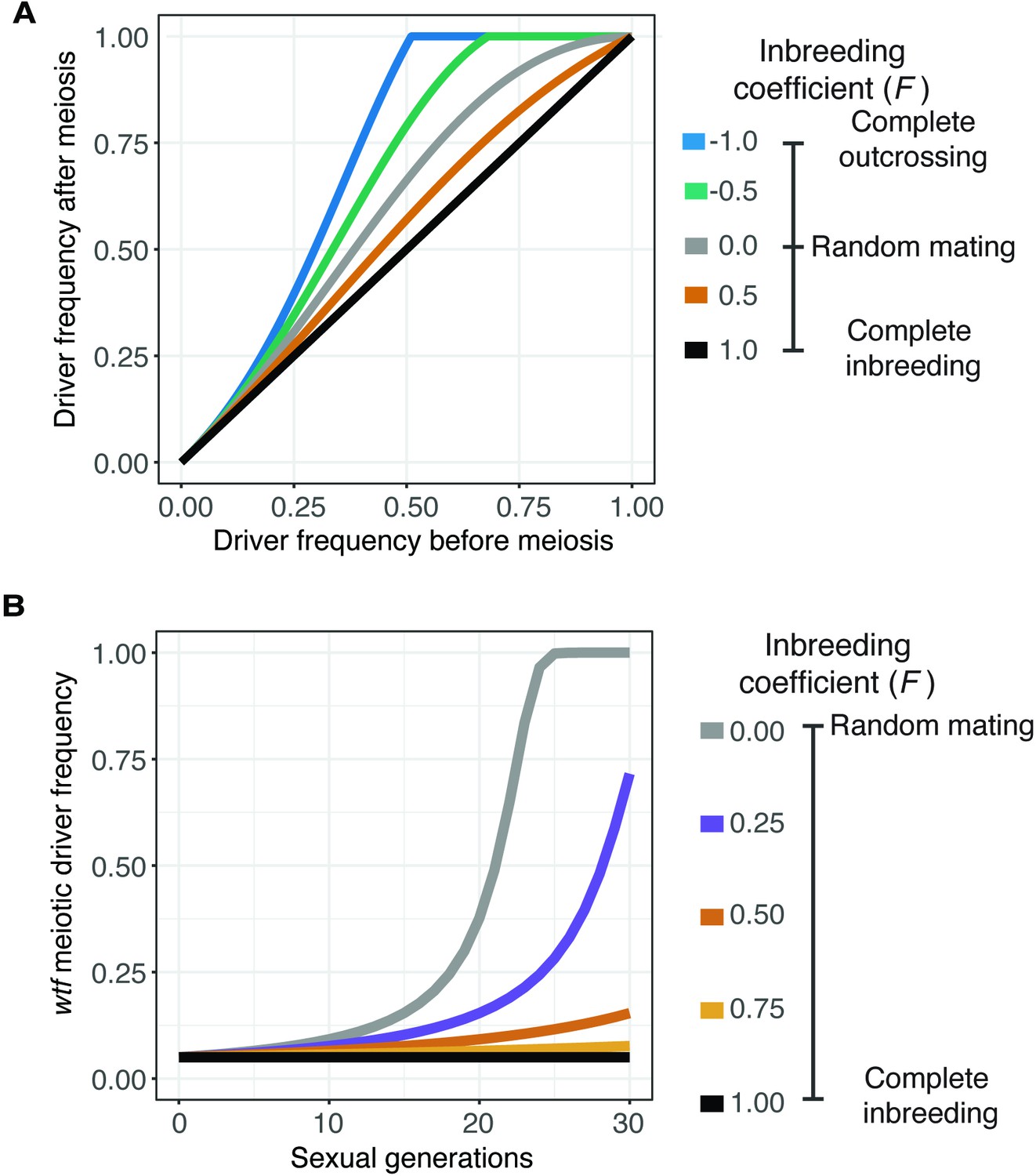
Inbreeding is predicted to slow the spread of a wtf driver.
We assumed a 0.98 transmission bias favoring the wtf driver and a fitness of 0.51 in wtf+/wtf- heterozygotes. We assumed that homozygote fitness is 1. We simulated the spread of a wtf driver for 30 generations. (A) Change of wtf meiotic driver frequency after a single meiosis assuming varying levels of inbreeding. (B) The spread of a wtf driver in a population over time assuming varying levels of inbreeding.
We next wanted to consider the spread of a wtf driver under conditions in which genetic drift could occur (Figure 3—figure supplement 1B and C). To do this, we simulated populations of different sizes (10–100,000 total individuals) that started with one driver. We followed the population for 1000 generations of mating and spore formation. We randomly selected surviving ‘haploids’ to populate the next generation to keep the population size fixed. We assumed that all genotypes have equal fitness during haploid cell growth. For mathematical simplicity, we assumed complete drive and a corresponding fitness of 0.5 in heterozygous diploids. We again assumed that both types of homozygous diploids had a fitness of 1. We also varied the inbreeding coefficient from 0 (random mating) to 1 (all matings generate homozygotes). Surprisingly, we found that the probability of a driver’s success was related to population size, similar to the recent results of Martinossi-Allibert et al., 2021. Specifically, the driver was most likely to be maintained in the smaller populations and in populations with more random mating due to the driver’s positive effect on its own allele transmission (Figure 3—figure supplement 1C). In larger populations in which the drivers started at a lower initial frequency, the drive allele generally took a long time to increase its frequency compared to the alternate allele, or it was lost due to drift. This was especially true when inbreeding coefficients were high (Figure 3—figure supplement 1C).
Inbreeding and linked deleterious alleles can suppress the spread of wtf drivers
We next wanted to test if our predictions reflect the behavior of wtf drive alleles in a laboratory population of Sp cells over many generations. To do this, we constructed an experimental evolution system employing the GFP and mCherry fluorescent markers described above to measure changes in allele frequencies in a population over time using cytometry. To mark drive alleles, we linked the fluorescent markers with the Sk wtf4 driver and integrated the whole construct at the ura4 locus in Sp (Nuckolls et al., 2017). For non-driving alleles, we used GFP or mCherry integrated at the ura4 locus without a linked wtf gene. We call the non-wtf alleles ‘empty vector’. We started the experimental evolution populations with a defined ratio of GFP- and mCherry-expressing cells. We then induced a subset of the population to mate and sporulate followed by collection and culturing of the progeny (spores). From these cells, we remeasured GFP and mCherry frequencies using flow cytometry, and we initiated the next round of mating and meiosis (Figure 4A).
Figure 4 with 2 supplements see all
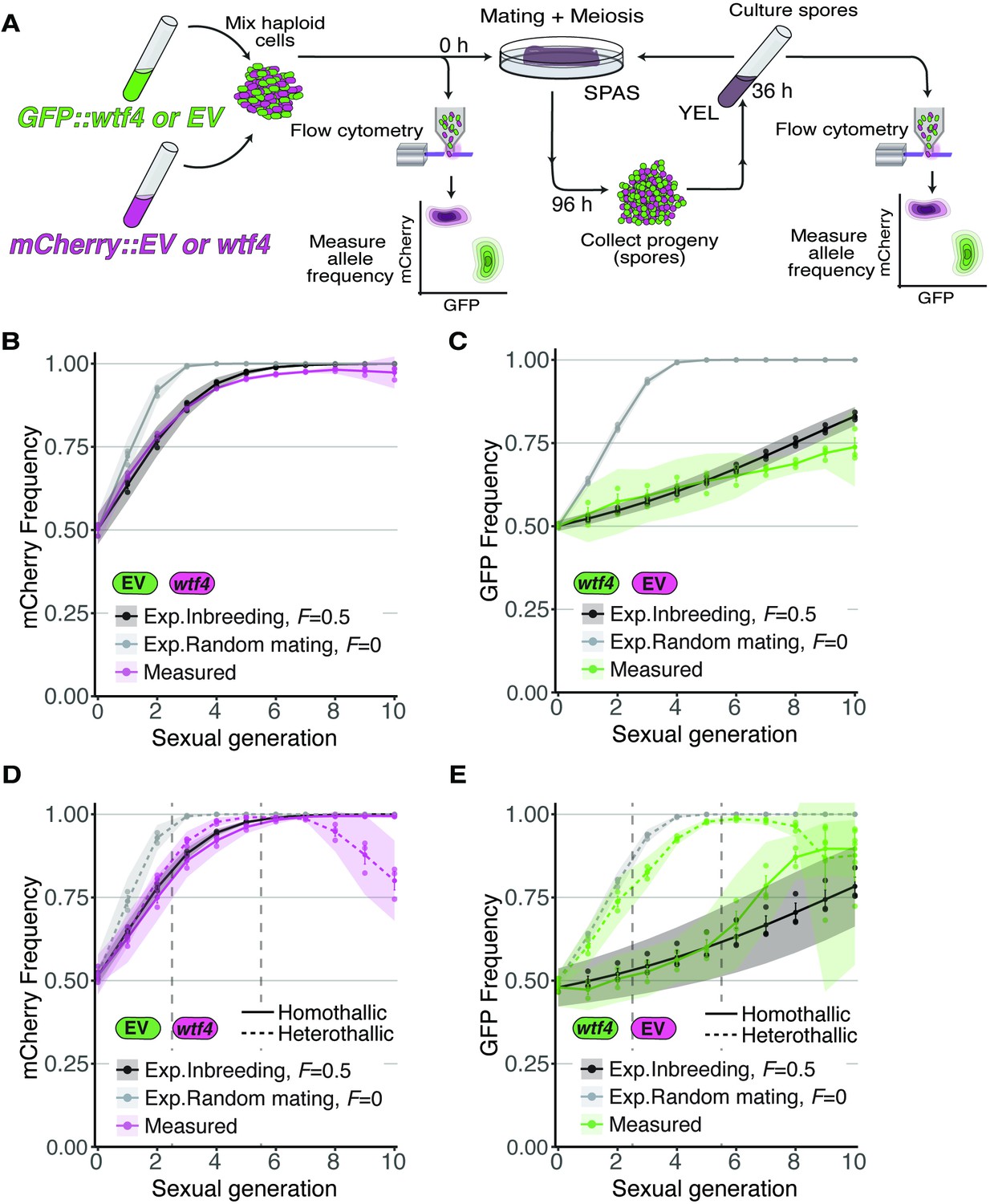
Inbreeding slows the spread of the wtf4 meiotic driver in homothallic strains.
(A) Experimental strategy to monitor allele frequency through multiple generations of sexual reproduction. GFP (green) and mCherry (magenta) markers are used to follow empty vector (EV) alleles or the wtf4 meiotic driver. Starting allele frequencies and allele frequencies after each round of sexual reproduction were monitored using cytometry. (B) Homothallic population with mCherry marking wtf4 and GFP marking an EV allele. Allele dynamics were predicted using drive and fitness parameters described in the text assuming an inbreeding coefficient of 0.5 (black lines) and random mating (inbreeding coefficient of 0; gray lines). The individual spots represent biological replicates and the shaded areas around the lines represent 95% confidence intervals. (C) Same experimental setup as in (B), but with mCherry marking the EV allele and GFP marking wtf4. (D–E) Repeats of the experiments shown in (B) and (C) with two alterations. First, these experiments tracked heterothallic populations (dotted lines) in addition to homothallic cells (solid lines). Second, the populations were sorted by cytometry at generations 3 and 5 (vertical long-dashed lines) to remove non-fluorescent cells.
Because our experiments rely on comparing the frequency of GFP- and mCherry-expressing cells over time, we needed to test the relative fitness of the markers. We found that both fluorescent markers were lost from all our experimental populations over time (Figure 4—figure supplement 1A-B). This was likely because insertion of the markers disrupted the ura4 gene and cells that excised the marker reverted the ura4 mutation and thereby gained a fitness benefit. We therefore only considered fluorescent cells for our analyses and stopped the experiments when more than 95% cells lacked a fluorescent marker. In addition, in one set of experiments we also sorted cells at defined timepoints to remove non-fluorescent cells from our populations (Figure 4D–E, Figure 4—figure supplement 1B and Figure 4—figure supplement 2C-D, described below).
To assay for potential differences in the fitness costs of GFP and mCherry markers, we carried out our analyses in two control populations without drive. One control population lacked the Sk wtf4 driver while the other had Sk wtf4 linked to both fluorescent markers. For both types of controls, we analyzed homothallic (inbreeding coefficient ~0.5) and mixed heterothallic (inbreeding coefficient ~0) cell populations (Figure 1D). We found in most cases that the number of mCherry-expressing cells increased at the expense of GFP-expressing cells over time (Figure 4—figure supplement 2A-D). The notable exception was in heterothallic populations containing Sk wtf4 linked to both fluorophore alleles, where we did not observe a different cost of the GFP allele compared to mCherry (Figure 4—figure supplement 2D). The origin of the differential fitness between mCherry and GFP alleles and why this cost was not observed in the one heterothallic population are both unclear. We did not determine the cause of the differences between them.
To allow us to predict expected allele frequencies more accurately, we wanted to obtain a gross estimate of the fitness cost of the GFP-marked alleles relative to the mCherry-marked alleles in our experiments. To do this, we used the first six generations of data from our control crosses (Figure 4—figure supplement 2) to fit a maximum likelihood model in which all parameters were fixed except the fitness values of GFP/mCherry heterozygotes and GFP/GFP homozygotes. We found that the fitness cost of the GFP in homozygotes was 0.234 (see Materials and methods). We found the dominance of the GFP cost was 0.083 (low fitness cost of GFP in GFP/mCherry heterozygotes). We then used these costs, calculated from our controls without meiotic drive, to calculate expected values in our experimental analyses in which drive can occur (Figure 4B–E).
For our experiments competing Sk wtf4 with an empty vector allele, we first assayed populations in which the alleles both started at 50% frequency. In homothallic (inbreeding coefficient ~0.5) populations, we observed that wtf4 alleles spread in the population over several generations of sexual reproduction. The driver spread faster when linked to mCherry than when linked to GFP, presumably due to the aforementioned fitness costs linked to GFP (Figure 4B–C). In both cases, the rate of spread of the allele was very close to our model’s predictions if we assumed an inbreeding coefficient of 0.5 (black lines, Figure 4B–C) and differed considerably from the model’s predictions assuming random mating (inbreeding coefficient = 0; gray lines, Figure 4B–C).
We saw similar spread of wtf4 in homothallic populations in a set of repeat experiments in which we sorted the cell populations twice to remove non-fluorescent cells (Figure 4D and E). In these experiments, we also assayed mixed heterothallic populations with an equal mix of GFP- and mCherry-marked cells from both mating types. As described above, these mixed heterothallic populations show random mating (inbreeding coefficient ~0) between GFP- and mCherry-labeled cells (Figure 1D). In the mixed heterothallic populations, the wtf4 driver spread significantly faster than in homothallic cells. In generations 1–6, the spread of wtf4 was very similar to that predicted by our model if we assumed random mating (inbreeding coefficient = 0). In later generations, our observations did not fit the model well. We suspect extensive loss of fluorescent cells, especially those with mCherry, and the resulting decrease in population size could contribute to this effect (Figure 4D and E; Figure 4—figure supplement 1).
We compared our data to a model in which driver heterozygotes have a fitness of 0.51, but we also considered variants of the model in which heterozygotes have fitness greater than 0.5, as can occur with spore killers in Podospora anserina (Vogan et al., 2021; Martinossi-Allibert et al., 2021). In S. pombe, an increase in driver heterozygote fitness could occur if the driving alleles benefit from drive beyond the benefits gained directly by killing spores bearing the alternate allele. For example, the surviving meiotic products could theoretically gain fitness during spore development by scavenging increased resources from the killed meiotic products (Nauta and Hoekstra, 1993). We found that increasing heterozygote fitness beyond 0.51 decreased the fit of our data to the model (Figure 5—figure supplement 2), suggesting wtf drivers do not gain additional benefits beyond killing spores bearing the alternate allele.
Overall, our results demonstrate that our population genetics model with driver heterozygote fitness at 0.51 is good at describing the spread of wtf4 in our experimental population, particularly in the first few generations. Our results also confirm that inbreeding coefficients near 0.5 slow, but do not stop, the spread of drivers in a population.
Meiotic drivers tend to accumulate linked deleterious alleles in nature (Atlan et al., 2004; Dyer et al., 2007; Finnegan et al., 2019; Fishman and Saunders, 2008; Higgins et al., 2018; Lyon, 2003; Olds-Clarke, 1997; Schimenti et al., 2005; Unckless et al., 2015; Wilkinson and Fry, 2001; Wu, 1983). While the linkage of individual drivers to deleterious alleles in S. pombe has not been extensively investigated, driving alleles in the Sk isolate are linked to a chromosomal translocation that decreases fitness in heterozygotes (Zanders et al., 2014). Similar chromosomal rearrangements involving chromosome 3, which houses most wtf genes, are common in S. pombe, so it is likely drivers are frequently linked to rearrangements (Bowen et al., 2003; Brown et al., 2011; Avelar et al., 2013). We therefore used the population genetic model to calculate the ability of a driver to spread when tightly linked to alleles with fitness costs ranging from 0 to 0.8. We also varied the inbreeding coefficient from 0 (random mating) to 1 (no heterozygotes are produced).
We found that, in the absence of additional linked costs, wtf drivers are predicted to spread in a population at all initial frequencies greater than 0 (Figure 5A). As described above, this spread is slowed by inbreeding, but is not stopped until inbreeding coefficients reach 1 (no heterozygotes are produced). When the driver is burdened by additional fitness costs, it can still spread in a population. Importantly, however, as the fitness costs of linked deleterious alleles increase, the driver must start at a higher initial frequency to spread. If the fitness costs are recessive or close to recessive (dominance coefficient h near 0), a driver can invade at low frequencies in a randomly mating population, but a driver would require a higher initial frequency to spread in an inbreeding population (inbreeding coefficients > 0; Figure 5A, Figure 5—figure supplement 1A). If the fitness costs are partially dominant (50% dominance), the drivers require a higher initial frequency to spread, even with random mating (Figure 5—figure supplement 1B).
Figure 5 with 2 supplements see all

Inbreeding purges wtf drivers with linked deleterious alleles.
(A) Modeling the predicted impacts of inbreeding, the fitness of the driving haplotype, and the initial frequency of the driver on the spread of a wtf driver linked to a deleterious allele with low dominance (h = 0.083) in a population. The circle indicates the predicted initial frequency necessary for the GFP:wtf4+ allele to spread in a population when mated at standard (1×) density where F = 0.5. The diamond indicates the predicted initial frequency necessary for the GFP:wtf4+ allele to spread in a population when mated at low (0.1×) density where F = 0.8–0.95 measured in Figure 1—figure supplement 2C. (B) Experimental analyses of the impacts of inbreeding and the initial driver frequency on the spread of the GFP:wtf4+ allele in a population. A single biological replicate was used for each initial frequency and inbreeding condition.
In finite populations in which drift can occur, we also observed that linked costs could limit the maintenance of a driver particularly in populations that inbreed (inbreeding coefficients > 0; Figure 5—figure supplement 1C,D). This is in line with previous modeling and can be explained because the cost of the deleterious allele is fixed, but the benefit a driver gains from drive is frequency dependent (Drury et al., 2017; Martinossi-Allibert et al., 2021; Nauta and Hoekstra, 1993).
We next tested these predictions experimentally using the Sk wtf4 allele linked to GFP in homothallic cells. As described above, the GFP allele is linked to an unknown deleterious trait (estimated 1.9% and 23.4% cost in heterozygotes and homozygotes, respectively). We varied the inbreeding coefficients of the populations by assaying cells mated at 1× and 0.1× density. As reported above, homothallic cells mated at 1× density exhibit an inbreeding coefficient of 0.5–0.57, but that is increased to 0.8–0.95 by mating the cells at low (0.1×) density (Figure 1D, Figure 1—figure supplement 2B and C ). Consistent with the predictions of our model, we observed in the experimental populations that the driver failed to spread when the initial frequency was less than 0.25 (Figure 5B). When the wtf4:GFP allele was found in roughly half of the population, it could spread when the inbreeding coefficient was low but decreased in frequency when the inbreeding coefficient was increased (Figure 5B). Similar, but less dramatic, effects were observed at higher initial frequencies of the wtf4:GFP allele. Altogether, our experimental analyses are consistent with the predictions of our model and show that both inbreeding and linked deleterious alleles can impede the spread of a wtf meiotic driver.
Discussion
Natural variation in mating phenotypes in S. pombe
Mating phenotypes, particularly the outcrossing rate, are key parameters that affect the evolution of species (Muller, 1932; Otto and Lenormand, 2002). We sought to explore mating phenotypes in S. pombe to better understand the evolution of the wtf gene family found in this species. Although genetic variation within S. pombe is limited, past studies found variation in mating efficiency and uncovered genetic diversity of the mating-type locus (Jeffares et al., 2015; Nieuwenhuis et al., 2018; Rhind et al., 2011; Singh and Klar, 2002). In this work, we assayed mating in an array of homothallic S. pombe natural isolates under a variety of laboratory conditions. Similar to previous work, we found Sp mating efficiency close to 40% and observed variable mating efficiencies for natural isolates (Merlini et al., 2016; Seike et al., 2019a). In addition, we quantified the propensity of natural isolates to undergo same-clone mating when given the opportunity to mate with non-clonally related cells. We found this trait, as measured using an inbreeding coefficient, was variable between natural isolates and could be affected by cell density or available sexual partners.
All of the S. pombe natural isolates we studied are homothallic and thus capable of same-clone mating. Despite this, we found that all isolates underwent some non-same-clone mating. In addition, some isolates, like Sk, showed considerable non-same-clone mating (inbreeding coefficient near 0) under standard mating conditions. This provides additional data supporting homothallism is compatible with outcrossing between non-clonally related isolates (Attanayake et al., 2014). In addition, S. pombe asci undergo a programmed degeneration process (endolysis) shortly after spore formation (Encinar del Dedo et al., 2009). This presumably frees spores to potentially distribute (in wind, water, or associated with animals) separate from the other spores produced in the same meiosis. The physical independence of S. pombe spores could also facilitate outcrossing in this homothallic fungus (Billiard et al., 2012).
We did not definitively identify the molecular mechanisms underlying the variation in mating phenotypes we observed. Our data is, however, consistent with a model in which less frequent mating-type switching in the Sk isolate contributes to more random mating in Sk than in the common lab isolate, Sp. Specifically, if switching is less frequent in Sk, sibling cells are less likely to be compatible to mate. Incompatibility of sibling cells opens the possibility for mating with other, perhaps non-clonally derived, cells in the population. Singh and Klar were the first to propose that Sk switched less frequently than Sp when they noticed less of the DNA break that initiates switching (Singh and Klar, 2002). We discovered a large, nested insertion of transposon sequences in the mating-type locus of Sk, and we posit that this insertion could contribute to reduced DNA break formation and, potentially, decreased mating-type switching. It is important to note, however, that not all strains that mate randomly share this transposon insertion. We also stress that, as in previous work (e.g., Miyata and Miyata, 1981), we did not directly assay switching rates and instead used mating events to infer information about switching. The long shmoos we observed in Sk may also contribute to more random mating in this isolate, as the long shmoo may increase the available number of partners within range.
Additional previously described natural variation that we did not functionally explore may also contribute to differences in inbreeding propensity in S. pombe. For example, heterothallic natural isolates are predicted to exclusively undergo non-same-clone mating with cells of the opposite mating type (Jeffares et al., 2015; Nieuwenhuis et al., 2018). In addition, homothallic isolates with atypical mating-type loci with extra copies of the mat cassettes could grow into populations that are biased toward one mating type (Nieuwenhuis and Immler, 2016). Indeed, we analyzed the presumably expressed mating-type locus (mat1) in several isolates for which we had nanopore sequencing data and found an approximate 3:1 excess of the h+ allele in FY29033 (Figure 2—figure supplement 2C). The excess of one mating type is predicted to also facilitate non-same-clone mating.
It is important to note that our study does not address the actual frequency of outcrossing in S. pombe populations in the wild. Very little is known about the ecology of fission yeast, including how frequently genetically distinct isolates are found in close enough proximity to mate (e.g., closer than ~40 µm apart) (Jeffares, 2018). Outcrossing rates have been estimated using genomic data, but those estimates generally assume both that heterozygous recombination rates will match those observed in pure Sp and that allele transmission is Mendelian (Farlow et al., 2015; Tusso et al., 2019). Although these genomic estimates are reasonable, neither of these assumptions is consistent with empirical analyses (Bravo Núñez et al., 2020b; Hu et al., 2017; Zanders et al., 2014). These assumptions have, therefore, likely led to an underestimation of the true outcrossing rate.
The effect of mating-type phenotypes on the spread of wtf meiotic drivers
To understand the evolution of the wtf drive genes, it is not necessarily essential to understand how frequently significantly diverged natural isolates, like those assayed in this work, mate. Instead, it is important to understand how often a driver is found in a heterozygous state. We suspect that heterozygosity for wtf drivers does not absolutely require outcrossing between more distantly related strains. This is because the wtf gene family, particularly the genes involved in meiotic drive, exhibit extremely rapid evolution. Even though genetic diversity within S. pombe is low (<1% average DNA sequence divergence in non-repetitive regions), the wtf genes present in different isolates tend to be largely distinct (Eickbush et al., 2019; Hu et al., 2017; Jeffares et al., 2015; Rhind et al., 2011). The number of wtf genes per isolate varies from 25 to 38 wtf genes (including pseudogenes), and even genes found at the same locus can be dramatically different (e.g., <61% coding sequence identity between alleles of wtf24) (Eickbush et al., 2019). For example, wtf22 is a predicted pseudogene in one strain, a predicted antidote in another strain, and is predicted to encode distinct drivers (i.e., mutually killing) in two more strains. There is only one wtf locus where all four strains that were surveyed each contain a meiotic driver, wtf4 (Eickbush et al., 2019). Still, we do not consider this a fixed driver because the sequence of wtf4 is different in each strain, which, in all cases tested, leads to a distinct drive phenotype (Bravo Núñez et al., 2018; Bravo Núñez et al., 2020a; Bravo Núñez et al., 2020b; Eickbush et al., 2019; Hu et al., 2017). For example, because Sk wtf4 and Sp wtf4 have different sequences, the antidote of Sk wtf4 does not neutralize Sp wtf4 and vice versa (Bravo Núñez et al., 2020a). The rapid evolution of wtf genes is driven largely by non-allelic gene conversion within the family and expansion or contraction of repetitive sequences within the coding sequences of the genes (Eickbush et al., 2019).
Because wtf genes generally provide no protection against wtf drivers with distinct sequences, the variation in wtf gene sequences has profound consequences (Bravo Núñez et al., 2018; Bravo Núñez et al., 2020a; Hu et al., 2017). Even small sequence changes in wtf drivers can cause the birth and death of drivers. When a cell bearing a novel wtf driver mutation mates with a cell without the mutation, the driver is heterozygous, and thus, drive can occur and the novel allele can potentially spread through the otherwise largely homogeneous population. Given fission yeast cells have no inherent mobility, the novel drive alleles could arise within small isolated subpopulations (demes) in which drivers have an increased possibility of establishing, as was formally described by Martinossi-Allibert et al., 2021.
Previous work assayed the strength of drive and the associated fitness reduction due to heterozygous wtf drivers (Bravo Núñez et al., 2018; Bravo Núñez et al., 2020a; Hu et al., 2017; Nuckolls et al., 2017). Those data, along with the inbreeding coefficients measured in this study, allowed us to mathematically model the spread of a wtf meiotic driver in an S. pombe population. Our modeling showed that the inbreeding coefficients we observed in S. pombe could slow the spread of a wtf driver. In the absence of drift, however, even the highest inbreeding coefficients we observed in S. pombe do not halt the spread of a driver, except in cases where the driver is found in low frequencies and linked to a deleterious allele. Given the tractability of S. pombe, we were also able to test the predictions of the model experimentally. Overall, our experimental results were quite similar to the model’s predictions discussed above. This suggests that our model encompasses all critical parameters. In addition, our experiments show how the wtf drivers can persist and spread in S. pombe, even if outcrossing is infrequent. The variation of mating phenotypes also indicates that the rate of spread of a wtf driver is expected to vary between different populations of S. pombe.
Overall, our results are consistent with previous empirical and modeling studies of meiotic driver dynamics in populations. For example, like our fortuitously deleterious GFP allele, meiotic drivers are often linked to deleterious alleles that can hitchhike with the driver (Atlan et al., 2004; Dyer et al., 2007; Finnegan et al., 2019; Fishman and Saunders, 2008; Higgins et al., 2018; Lyon, 2003; Olds-Clarke, 1997; Schimenti et al., 2005; Unckless et al., 2015; Wilkinson and Fry, 2001; Wu, 1983). The added costs reduce the spread of drivers, which can lead a population to harbor a driver at stable intermediate frequency (Dyer and Hall, 2019; Finnegan et al., 2019; Fishman and Kelly, 2015; Hall and Dawe, 2018; Manser et al., 2011). Additionally, inbreeding can be selected as it increases fitness in a population when a driver is recessive lethal (cost ~1, h = 0), such as in synthetic drive systems (Bull, 2016).
S. pombe as a tool to experimentally model complex drive dynamics
To conclude, we would like to highlight the potential usefulness of the S. pombe experimental evolution approach developed for this study. With this system, we were able to observe the effects of altering allele frequencies, inbreeding rate, and fitness of a driving haplotype. In the future, this system could be used to experimentally explore additional questions about drive systems. For example, one could experimentally model meiotic drivers that bias sex ratios by linking the driver to the mating-type locus in a heterothallic population. In addition, one could explore the evolution of complex multi-locus drive systems employing combinations of multiple wtf meiotic drivers or drivers and suppressors. This tool could lead to novel insights about natural drivers, but it may also be particularly useful for exploring potential evolutionary trajectories of artificial gene drive systems (Burt and Crisanti, 2018; Drury et al., 2017; Price et al., 2020; Wedell et al., 2019).
Materials and methods
Generation of Ura4-integrating vectors and fluorescent strains
Request a detailed protocolWe introduced the fluorescent genetic markers into the genome using plasmids that integrated at the ura4 locus. To generate the integrating plasmids, we first ordered gBlocks from IDT (Coralville, IA) that contained mCherry or GFP under the control of a TEF promoter and ADH1 terminator (Hailey et al., 2002; Sheff and Thorn, 2004). We digested the gBlocks with SpeI and ligated the GFP cassette into the SpeI site of pSZB331 and the mCherry cassette into the SpeI site of pSEZB332 (alternate clone of pSZB331; Bravo Núñez et al., 2020a; Bravo Núñez et al., 2020b) to generate pSZB437 and pSZB882, respectively. We then linearized the plasmids with KpnI and transformed them into S. pombe using the standard lithium acetate protocol (Schiestl and Gietz, 1989). We independently transformed the isolates GP50 (S. pombe), S. kambucha, FY28974, FY28981, FY29022, FY29033, FY29043, and FY29044. We were unsuccessful in transforming FY28969, FY29048, and FY29068. FY29033 was not included in the inbreeding analyses due to its proclivity to clump. The homothallic and heterothallic strains carrying mCherry or GFP were transformed using the same method.
To add Sk wtf4 to the Sp genome, we again used a ura4-integrating plasmid. To generate this plasmid, we amplified Sk wtf4 from SZY13 using the oligos 688 and 686. We digested the amplicon with SacI and ligated into the SacI site of pSZB332 to generate pSZB716 (Bravo Núñez et al., 2020a; Bravo Núñez et al., 2020b). We then separately introduced the GFP and mCherry gBlocks into the SpeI site of pSZB716 to generate pSZB904 and pSZB909, respectively. We introduced the resulting plasmids into yeast as described above.
Crosses
Request a detailed protocolWe performed crosses using standard approaches (Smith, 2009). We cultured each haploid parent to saturation in 3 mL YEL (0.5% yeast extract, 3% dextrose, and 250 mg/L adenine, histidine, leucine, lysine, and uracil) for 24 hr at 32°C. We then mixed an equal volume of each parent (700 μL each for individual homothallic strain, 350 μL for heterothallic parents), pelleted and resuspended in an equal volume of ddH2O (1.4 mL total), then plated 200 μL on SPA (1% glucose, 7.3 mM KH2PO4, vitamins, and agar) for microscopy experiments or SPAS (SPA +45 mg/L adenine, histidine, leucine, lysine, and uracil) for genetics experiments. We incubated the plates at 25°C for 1–4 days, depending on the experiment (see figure legends for exact timing). When we genotyped spore progeny, we scraped cells off of the plates and isolated spores after treatment with B-Glucuronidase (Sigma) and ethanol as described in Smith, 2009.
Iodine staining
Request a detailed protocolWe grew haploid isolates to saturation in 3 mL YEL overnight at 32°C. We washed the cells once with ddH2O then resuspended them in an equal volume ddH2O. We then spotted 10 μL of each strain onto an SPAS plate, which we then incubated at 25°C for 4 days prior to staining with iodine (VWR iodine crystals) vapor (Forsburg and Rhind, 2006).
Mating-type locus assembly and PCR
Request a detailed protocolWe used mate-pair Illumina sequencing reads to assemble the mating-type locus of S. kambucha with previously published data (Eickbush et al., 2019). We assembled the mating-type locus using Geneious Prime software (https://www.geneious.com; last accessed March 18, 2019) using an analogous approach to that described to assemble wtf loci (Eickbush et al., 2019).
DNA extraction for nanopore sequencing
Request a detailed protocolTo extract DNA for nanopore sequencing, we used a modified version of a previously developed protocol (Jain et al., 2018). We pelleted 50 mL of a saturated culture and proceeded as described, with the addition of 0.5 mg/mL zymolyase to the TLB buffer immediately prior to use.
Nanopore sequencing and assembly
Request a detailed protocolWe used a MinION instrument and R9 MinION flow cells for sequencing. For library preparation, we used the standard ligation sequencing prep (SQK-LSK109), including end repair using the NEB End Prep Enzyme, FFPE prep using the NEB FFPE DNA repair mix, and ligation using NEB Quick Ligase. We did not barcode samples and thus used each flow cell for a single genome. We used guppy v2.1.3 for base calling. We removed sequencing adapters from the reads using porechop v0.2.2 and then filtered the reads using filtlong v0.2.0 to keep the 100× longest reads. We then error corrected those reads, trimmed the reads and de novo assembled them using canu v1.8 and the ovl overlapper with a predicted genome size of 13 mb and a corrected error rate of 0.12 (Koren S et al., 2017). Base called reads are available as fastq files at the SRA under project accession number PRJNA732453.
In order to count allele frequency within the active mat locus, we mapped raw reads back to the corresponding de novo assembly using graphmap v0.5.2 and processed using samtools v1.12 (Li et al., 2009; Sović et al., 2016). We then visually observed the reference-based assemblies using IGV v2.3.97 to count the number of h + and h- alleles present at the active mating type locus with anchors to unique sequence outside the mat locus (Robinson et al., 2011).
Measuring inbreeding coefficients by microscopy
Request a detailed protocolWe mixed haploid parents (a GFP- and an mCherry-expressing strain) in equal proportions on SPA as described above. We then left the plate to dry for 30 min and then took a punch of agar from the plate using a 1271E Arch Punch (General Tools, Amazon). We then inverted the punch of agar into a 35 mm glass bottomed dish (No 1.5 MatTek Corporation). We used this sample to count the initial frequency of the two parental types. We then imaged a second punch of agar taken from the same SPA plate after 24 hr incubation at 25°C for homothallic cells and 48 hr for heterothallic cells. Each biological replicate was constituted by a separate cross.
To image the cells, we used an AXIO Observer.Z1 (Zeiss) widefield microscope with a 40× C-Apochromat (1.2 NA) water-immersion objective. We excited mCherry using a 530–585 nm bandpass filter which was reflected off an FT 600 dichroic filter into the objective and collected emission using a long-pass 615 nm filter. To excite GFP, we used a 440–470 nm bandpass filter, reflected the beam off an FT 495 nm dichroic filter into the objective and collected emission using a 525–550 nm bandpass filter. We collected emission onto a Hamamatsu ORCA Flash 4.0 using µManager software. We imaged at least three different fields for each sample as each technical replicate.
We used cell shape to identify mated cells (zygotes and asci) and used fluorescence to identify the genotype of each haploid parent. To measure both fluorescence and the length of asci, we used Fiji (https://imagej.net/Fiji) software to hand-draw five pixel-width lines through the length of each zygote or ascus. After subtracting background using a rolling ball background subtraction with width 50 pixels, we then measured the average intensity for the GFP and mCherry channels. When measuring the log10 ratio of GFP over mCherry, the mCherry homozygotes have the lowest ratio, homozygotes for GFP the highest ratio, and heterozygotes intermediate.
To calculate the inbreeding coefficient, we used the formula F = 1 − (observed heterozygotes/expected heterozygotes). We used Hardy-Weinberg expectations to calculate the expected frequency of heterozygotes (2p(1p)) for each sample, where ‘p’ is the fraction of mCherry+ cells and (1-p) is the fraction of GFP+ cells measured prior to mating (Hartl and Clark, 2007).
Visualizing mating and meiosis using time-lapse microscopy
Request a detailed protocolFor time-lapse imaging of cells mated at 1× density (Figure 2C), we prepared cells using the agar punch method described above. For cells at 0.25× density (Figure 2B), we used the same approach, except we cultured cells in 3 mL EMM (14.7 mM C8H5KO4, 15.5 mM Na2HPO4, 93.5 mM NH4Cl, 2% w/v glucose, salts, vitamins, minerals) then washed three times with PM-N (8 mM NA2HPO4, 1% glucose, EMM2 salts, vitamins, and minerals) before plating cells to SPA. While imaging the cells, we added a moistened kimwipe to the MatTek dish to maintain humidity. We sealed the dish lids on with high-vacuum grease (Corning). We imaged cells using either a Ti Eclipse (Nikon) coupled to a CSU W1 Spinning Disk (Yokagawa), or a Ti2 (Nikon) widefield using the 60× oil immersion objective (NA 1.45), acquiring images every ten minutes for 24–48 hr, using a 5 × 5 grid pattern with 10% overlap between fields. The Ti Eclipse was used for one replicate each of the 1× crosses and the Ti2 was used for all remaining experiments. We used an Okolab stage top incubator to maintain the temperature at 25°C. For the Ti2 (widefield) data we excited GFP through a 470/24 nm excitation filter and collected through an ET515/30 m emission filter. For mCherry on this system, we excited through a 550/15 nm excitation filter and collected through an ET595/40 m emission filter. For the Ti Eclipse (confocal) data, we excited GFP with a 488 nm laser and collected its emission through an ET525/36 m emission filter. For mCherry on this system, we excited with a 561 nm laser and collected through an ET605/70 m emission filter.
To monitor mating in 1× crosses (Figure 2C-E), we recorded the number of divisions and mating choice of the progeny of 286 cells until an expected mating efficiency for the population being filmed was attained. The expected mating efficiency was calculated from still images of the same crosses. We recorded two videos of each cross.
To monitor the number of divisions required before mating could occur in 0.25× cultures (Figure 2B), around 200 individual cells were monitored through the duration of the generation in which the first mating event occurred. If cells failed to mate, they were monitored throughout the duration of the movie. If a cell or its mitotic offspring interacted with a neighboring cell cluster, it was not included in the analysis. We recorded two videos for each isolate.
Calculation of mating efficiency
Request a detailed protocolWe calculated mating efficiency from microscopic images using the following formula:
where represents the number of zygotes, represents the number of asci, represents the number of free spores, and represents the number of vegetative cells (Seike and Niki, 2017).
Switching assay
Request a detailed protocolIn an attempt to directly observe mating-type switching, we used the strain TP220 (Jakočiūnas et al., 2013). This strain contains a dual reporter system with YFP under control of the h- cell-specific mfm3 promoter and CFP under control of the h + cell-specific map2 promoter. Cells were cultured for 24 hr in PM-N+ ade + leu and then plated to SPA+ ade + leu (at 0.5× density) or SPAS (at 1× density) (see figure legends). Plates were incubated at 25°C for 1 or 12 hr (SPA+ ade + leu and SPAS, respectively) before we prepared cells for microscopy using the agar punch method described above. Two microscopes were used for this analysis. In one case, a Nikon Ti microscope coupled to a Yokogawa CSU W1 spinning disc was used. CFP was excited with 445 nm and YFP was excited with 515 nm laser light. Cells were imaged with a 60× Plan Apochromat Objective (NA 1.4). CFP fluorescence was filtered through a 480/30 bandpass filter and YFP was filtered through an ET535/36 m bandpass filter. Fluorescence was recorded with an iXon DU897 EMCCD (Andor). In a separate experiment, a Nikon Ti2-E widefield microscope was used. Here, a bulb was filtered to excite CFP with a 440/20 nm bandpass filter while YFP was excited with a 510/25 nm bandpass filter. The cells were imaged with a 60× Plan Apochromat phase three objective (NA 1.4). The fluorescence of CFP was filtered through an ET472/24 nm bandpass filter and YFP was filtered through a 542/21 nm bandpass filter. Here, images were acquired with a Prime 95 sCMOS camera (Photometrics). In both datasets, images were acquired every 20 min for 24 hr. Images from these datasets were Gaussian blurred one pixel, then rolling ball background subtracted with a radius of 50 pixels. Sample movement was eliminated by registering the images using the plugin ‘StackRegJ_’ in Fiji. Subsections of the image were created by duplicating out 500 × 500 pixel regions from this large image. These were then Gaussian blurred one pixel again and brightness and contrast adjusted as needed to illustrate the fluorescence. Finally, these small fields of view were cropped again to yield the images in Figure 2—figure supplement 1.
Measuring inbreeding coefficients using genetics
Request a detailed protocolWe used a high-throughput system to genotype the progeny from each cross. First, we crossed two parental populations to generate spore progeny as described above. In addition to placing the mixed haploid cells on SPAS, we also diluted a subset of the mix and plated it onto YEAS (YEA +45 mg/L adenine, histidine, leucine, lysine, and uracil). We genotyped the colonies that grew on that YEAS plate to measure the starting frequency of each parental strain in the cross. We plated the spores produced by the cross on YEAS and grew them at 32°C for 4 days. We picked the colonies using a Qpix 420 Colony Picking System and cultured them in YEL for 24 hr at 30°C in 96-well round-bottom plates (Axygen). We then used a Singer RoTor robot to spot the cultures to YNP dropout and YEAS drug plates and incubated them at 32°C for 3 days. We then imaged the plates using an S&P robotics SPImager with a Canon EOS Rebel T3i camera. We analyzed each picture using the subtract background feature in Fiji and assigned regions of interest to the 384 spots where cells were pinned. We then measured the average intensity of each spot and classified cells as grown or not by a heuristic threshold. We genotyped some cross progeny manually using standard techniques due to robot unavailability, with indistinguishable results. A single cross was considered as one biological replicate.
We then inferred the frequency of mating between cells of distinct genotypes based on the frequency of recombinant progeny using a combination of either two or three unlinked genetic markers. If mating was random, we expect the progeny to reflect Hardy-Weinberg expectations (), where reflect the expected frequency of homozygotes and reflects the expected frequency of outcrossing. Homozygotes of either parental genotype can only produce offspring with the parental genotypes. If the two parental strains outcross to generate heterozygotes, they will make the parental genotypes and recombinant genotypes all in equal frequencies (2n total genotypes where n is the number of segregating markers). For our crosses with three markers, we therefore expected the true ‘observed’ frequency of progeny produced by outcrossing to be equal to the number of observed recombinants divided by 6/8. For our crosses with two unlinked markers, we divided by 2/4. We then calculated the inbreeding coefficient using the formula,
Zygote frequency expectation under inbreeding and different mating efficiencies
Request a detailed protocolWe calculated the expected zygote frequencies when isolates were mated with different isolates on SPA (see Measuring inbreeding coefficients by microscopy) using an additive model that incorporated mating efficiencies and inbreeding coefficients measured from the isogenic crosses. The model assumed that each strain contributes equally to the cross, and that they do not change their own mating in response to the mating partner.
We calculated the expected frequency of homozygotes for parental strain one as:
where the inbreeding coefficient is and the mating efficiency is for parental strain 1 (), considering its initial frequency . The expected heterozygote frequency is:
The expected fraction of homozygotes for parental strain two is:
Calculating expected allele frequencies after sexual reproduction
Request a detailed protocolTo model the expected changes in allele frequencies in a randomly mating population over time, we used the equations described by Crow, 1991. For nonrandomly mating populations, we included the ‘’ inbreeding coefficient in the equations, similar to Hartl and Clark, 2007. We assumed that wtf4 had a drive strength (‘') of 0.98 based on experimental observations (Nuckolls et al., 2017). We assumed the control allele exhibited Mendelian transmission ( = 0.5). Simulations for the spread of a driver in Figure 3 only considered drive and inbreeding coefficients. To simulate drive in fluorescent populations, the starting frequencies of each allele (i.e., ‘’) were determined empirically for each experiment using either traditional genetic approaches or cytometry. Predicted values were calculated from each biological replicate (independent cross), composed of three technical replicates measured via cytometry per cross. We assumed all genotypes had equal fitness as haploids. For relative fitness of diploids, we assigned mCherry/mCherry homozygotes a fitness of , regardless of whether they were EV/EV or wtf4/wtf4 homozygotes. In all but one cross (see below), we observed a fitness cost linked to the GFP alleles relative to mCherry alleles during sexual reproduction, regardless of wtf4. We therefore used our data (see below) to calculate 0.234 as the fitness cost of the GFP-linked variant. Because of that, we assigned a fitness value of 0.766 to GFP homozygotes, . We found the fitness cost linked to GFP had low dominance (see below) and thus assigned a fitness value of 0.98 for GFP/mCherry homozygous for wtf4 or empty vector, . For GFP/mCherry heterozygotes that were also heterozygous for wtf4, we assigned a fitness of (0.5) that accounts for the death of spores killed by drive (0.51) and the GFP cost (0.234) and dominance (0.083).
The calculation for allele frequency for a wtf meiotic driver in consecutive sexual cycles from haploid populations is:
where the mean fitness of the population at each generation (
When the fitness reduction in heterozygotes is only due to dead cells by drive with no additional costs, , the drivers spread under any initial frequency greater than 0 (Crow, 1991).
To determine the fitness cost of the GFP-linked variant that was present in most of our experiments, we used the L-BFGS-B algorithm to find a fitness that maximized the likelihood that our observed allele frequencies varied only due to the linked cost of GFP () and dominance () in the first six generations of the control experiments shown in Figure 4—figure supplement 2 (Byrd et al., 1995). To do this, we used the mle function from the R stats4 package (Team, 2019). We assumed the fitness cost alters the relative fitness of both homozygotes and heterozygotes . The fitting was done using only the initial six generations due to a rapid loss of fluorescent cells from seven to ten generations (Figure 4—figure supplement 1).
To calculate the minimum initial frequency of driver required to spread in a population when linked to alleles with varying additional fitness costs, we use the additional linked cost ( and their dominance () associated to each genotype and solved using (Wolfram, 1987). For simplicity we also assumed complete transmission bias, . A wtf meiotic driver linked to a deleterious allele can spread under the condition (critical value) that
where is the initial frequency of a wtf driver, c is the cost linked to the driver, and h is the dominance coefficient. For this case the assigned relative fitness for homozygote carrying the wtf driver is .
Modeling driver success in finite populations
Request a detailed protocolTo determine the possibility of a meiotic driver to spread and be fixed in a finite population, we ran stochastic simulations using a Wright-Fisher model considering multiple population sizes. We assumed no fitness differences between genotypes during haploid cell growth, complete drive (k = 1), gamete killing proportional to drive in heterozygotes, no linked deleterious alleles, and non-overlapping generations. We used characters of ‘0’ for non-driving cells and ‘1’ for driving cells (Figure 3—figure supplement 1B). Initially the population starts with population size (N). We next sampled a fixed population size (n) with replacement, assuming infinite gamete supply used for mating (e.g., as if mitotic expansion of the population occurred prior to mating). In our simulations N = n. We sampled mating groups without replacement for an inbreeding population (Spop) with a fraction F and the rest of cells (n − Spop) mate randomly. Populations that mate randomly are proportional to Hardy-Weinberg genotype frequencies with approximated integer values. Homozygotes (‘0,0’ and ‘1,1’) produce four progeny (‘0,0,0,0’ and ‘1,1,1,1’, respectively), while heterozygotes produce two progeny that inherit the drive allele (‘1,1’). When a fitness cost is associated with a genotype, we decimated the gametic products in proportion to the cost. The collection of 0’s and 1’s after this process constituted the next generation. We repeated 1000 generations for 1000 iterations for each tested condition.
Measuring allele frequencies for experimental evolution analyses
Request a detailed protocolWe performed the crosses and collected spores as described above. We then started the next generation by culturing 60 µL of spores from each cross in each of three different wells with 600 µL fresh YEL media in 96 deep-well-round-bottom plates (Axygen) and cultured for 24 hr at 1200 rpm at 32°C. We then transferred 60 µL from each culture to a new plate with 600 µL YEL and cultured for 12–14 hr at 1200 rpm at 32°C. We then pooled the culture replicates in an Eppendorf tube, spun down, and resuspended them in an equal volume of ddH2O. We then took 100 µL of this sample to assay via cytometry (described below). We also plated 200 µL of each sample on SPAS plates and incubated at 25°C for 5 days to allow the cells to mate and sporulate.
To detect and quantify fluorescent cells via flow cytometry, we used the ZE5 Cell Analyzer (Bio-Rad). We spun down 100 µL of each culture, washed the cell pellet with water, spun down again, and resuspended the cells in 200 µL of 1× PBS (phosphate buffered saline) with 1.5 μL 4′,6-diamidino-2-phenylindole (DAPI, Sigma-Aldrich, 100 ng/mL). DAPI stains dead cells, so we considered DAPI-negative cells as live cells. To image DAPI, we used 355 nm laser excitation and a 447/60 nm detector. To image GFP, we excited using a 488 nm laser and detected emission with a 525/35 nm filter. To image mCherry, we excited using a 561 nm laser and detected emission with a 615/24 nm filter. We used 405 and 488 nm (FSC 405 and FSC 488) lasers for forward scatter and 488 nm laser for side scatter (SSC 488).
To quantify the frequency of GFP- or mCherry-positive cells, we analyzed the Flow Cytometry Standard files in R/Bioconductor using the packages FlowTrans and FlowClust (Lo et al., 2009). We first separated the cells that had round and uniform shape and similar granularity. This step allowed us to detect a more uniform population of single cells. We then discarded DAPI-positive cells. To determine the GFP- and mCherry-positive cells, we used limits for each channel. The limits varied throughout the experiment due to reconfiguration in the flow cytometer. For every measurement, we corrected with standard samples of cells that only expressed either GFP or mCherry. Fluorescent GFP- and mCherry-positive cells always showed non-overlapping cell populations. We quantified cells that were not classified as non-fluorescent cells.
Fluorescent marker loss in experimental evolution
Request a detailed protocolIn the experimental evolution experiments (Figures 4 and 5B, and Figure 4—figure supplement 2), a large proportion of cells lost their fluorescent marker over time (Figure 4—figure supplement 1A-B). We assume this is because we introduced the markers using an integrating plasmid that enters the genome following a single crossover event. Because of this, a single crossover can then pop the marker and the associated vector out of the genome. We repeatedly observed that the loss occurred faster with the mCherry markers. Consistent with this model, cells that lost fluorescence generally also lost the associated drug resistance marker present on the integrating vector.
We only considered fluorescent cells in our analyses. In the experiments (Figure 4B–C, Figure 4—figure supplement 1A-B, and Figure 5B), we extended the evolution up to 10 generations. In other experiments (Figure 4D–E and Figure 4—figure supplement 2C-D), we removed non-fluorescent cells by cell sorting after generations 2 and 5. To sort cells, we first collected and cultured spores as described above with the first culture done for 12 hr. We then transferred 60 µL of germinated cells into 600 µL fresh YEL media. We used three cultures for each experimental line and pooled all in equal amounts to have 1.4 mL of each line. We spun each sample down and resuspended the cells in 5 mL ddH2O prior to sorting. We removed non-fluorescent cells and retained GFP-positive (488 nm laser for excitation and a filter 507 nm) and mCherry-positive (561 nm laser for excitation and a 582 nm filter) cells using the laser the BD FACSMelody cell sorter software. We collected 1.2 million cells for each line into 1× PBS. We then spun down the cells and resuspended the pellets in 200 µL YEL. We then took 60 µL from each sample and diluted the cells into 600 µL YEL and continued with the time course as described above. This restored fluorescently labeled cells populations as expected for homothallic and heterothallic lines (Figure 4—figure supplement 1B). Cell sorting did not affect our results as we observed the same patterns in replicate experiments in which we did not remove the non-fluorescent cells (Figure 4).
Software flow cytometry data analysis and modeling scripts
Request a detailed protocolAnalysis performed to filter, measure, and compare flow cytometry with simulations are located in the Zanders Lab Github repository, https://github.com/Zanders-Lab/Diverse_mating_phenotypes_impact_the_spread_of_wtf_meiotic_drivers_in_S.-pombe; Zanders, 2021, http://www.stowers.org/research/publications/libpb-1625.
Data availability
Original data underlying this manuscript can be accessed from the Stowers Original Data Repository at http://www.stowers.org/research/publications/libpbxxxx. Base called reads are available as fastq files at the SRA under project accession number PRJNA732453.
-
NCBI BioProjectID PRJNA732453. NCBI BioProject.
-
NCBI Sequence Read ArchiveID SRX4224586. Mate-pair sequencing of S. kambucha lab strain SZY661.
References
-
Ace2p controls the expression of genes required for cell separation in Schizosaccharomyces pombeMolecular Biology of the Cell 16:2003–2017.https://doi.org/10.1091/mbc.e04-06-0442
-
Sex-ratio distorter of Drosophila simulans reduces male productivity and sperm competition abilityJournal of Evolutionary Biology 17:744–751.https://doi.org/10.1111/j.1420-9101.2004.00737.x
-
Sex, outcrossing and mating types: unsolved questions in fungi and beyondJournal of Evolutionary Biology 25:1020–1038.https://doi.org/10.1111/j.1420-9101.2012.02495.x
-
Lethal gene drive selects inbreedingEvolution, Medicine, and Public Health 2017:1–16.https://doi.org/10.1093/emph/eow030
-
Selfish DNA and breeding system in flowering plantsProceedings of the Royal Society of London. Series B 265:141–146.https://doi.org/10.1098/rspb.1998.0275
-
BookGenes in Conflict: The Biology of Selfish Genetic ElementsCambridge, MA: Belknap Press of Harvard University Press.
-
Gene Drive: Evolved and SyntheticACS Chemical Biology 13:343–346.https://doi.org/10.1021/acschembio.7b01031
-
A Limited Memory Algorithm for Bound Constrained OptimizationSIAM Journal on Scientific Computing 16:1190–1208.https://doi.org/10.1137/0916069
-
Why is Mendelian segregation so exact?BioEssays : News and Reviews in Molecular, Cellular and Developmental Biology 13:305–312.https://doi.org/10.1002/bies.950130609
-
Fitness consequences of a non-recombining sex-ratio drive chromosome can explain its prevalence in the wildProceedings. Biological Sciences 286:20192529.https://doi.org/10.1098/rspb.2019.2529
-
Killer Meiotic Drive and Dynamic Evolution of the wtf Gene FamilyMolecular Biology and Evolution 36:1201–1214.https://doi.org/10.1093/molbev/msz052
-
BookSetting up Schizosaccharomyces Pombe Crosses/MatingsCold Spring Harbor Protocols.https://doi.org/10.1101/pdb.prot091694
-
Meiotic drive reduces egg-to-adult viability in stalk-eyed fliesProceedings. Biological Sciences 286:20191414.https://doi.org/10.1098/rspb.2019.1414
-
Centromere-associated meiotic drive and female fitness variation in MimulusEvolution; International Journal of Organic Evolution 69:1208–1218.https://doi.org/10.1111/evo.12661
-
Genome Evolution in Outcrossing vs. Selfing vs. Asexual SpeciesMethods in Molecular Biology 1910:331–369.https://doi.org/10.1007/978-1-4939-9074-0_11
-
The control of septum formation in fission yeastGenes & Development 11:2939–2951.https://doi.org/10.1101/gad.11.22.2939
-
Genes that bias Mendelian segregationPLOS Genetics 10:e1004387.https://doi.org/10.1371/journal.pgen.1004387
-
Modeling the Evolution of Female Meiotic Drive in MaizeG3: Genes, Genomes, Genetics 8:123–130.https://doi.org/10.1534/g3.117.300073
-
The role of selfish genetic elements in eukaryotic evolutionNature Reviews. Genetics 2:597–606.https://doi.org/10.1038/35084545
-
Nanopore sequencing and assembly of a human genome with ultra-long readsNature Biotechnology 36:338–345.https://doi.org/10.1038/nbt.4060
-
The genomic and phenotypic diversity of Schizosaccharomyces pombeNature Genetics 47:235–241.https://doi.org/10.1038/ng.3215
-
Polymorphism of t -complex genes in European wild miceGenetical Research 44:39–46.https://doi.org/10.1017/S0016672300026239
-
Canu: Scalable and accurate long-read assembly via adaptiveGenome Research 27:722–736.https://doi.org/10.1101/gr.215087.116
-
Die vererburg von homothallie und heterothallie bei Schizosaccharomyces pombeComptes Rendus Des Travaux Du Laboratoire Carlsberg. Serie Physiologique 1:381–480.
-
The Sequence Alignment/Map format and SAMtoolsBioinformatics 25:2078–2079.https://doi.org/10.1093/bioinformatics/btp352
-
The Ecology and Evolutionary Dynamics of Meiotic DriveTrends in Ecology & Evolution 31:315–326.https://doi.org/10.1016/j.tree.2016.02.001
-
Transmission ratio distortion in miceAnnual Review of Genetics 37:393–408.https://doi.org/10.1146/annurev.genet.37.110801.143030
-
Polyandry and the decrease of a selfish genetic element in a wild house mouse populationEvolution; International Journal of Organic Evolution 65:2435–2447.https://doi.org/10.1111/j.1558-5646.2011.01336.x
-
Invasion and maintenance of meiotic drivers in populations of ascomycete fungiEvolution; International Journal of Organic Evolution 75:1150–1169.https://doi.org/10.1111/evo.14214
-
Mode of conjugation in homothallic cells of Schizosaccharomyces pombeThe Journal of General and Applied Microbiology 27:365–371.https://doi.org/10.2323/jgam.27.365
-
The evolution of mating-type switching for reproductive assuranceBioEssays : News and Reviews in Molecular, Cellular and Developmental Biology 38:1141–1149.https://doi.org/10.1002/bies.201600139
-
Repeated evolution of self-compatibility for reproductive assuranceNature Communications 9:1639.https://doi.org/10.1038/s41467-018-04054-6
-
Models for male infertility: the t haplotypesReviews of Reproduction 2:157–164.https://doi.org/10.1530/ror.0.0020157
-
Schizosaccharomyces liquefaciens n. Sp., eine gegen freie schweflige säure widerstandsfähige gärhefeMitt Gebiete Lebensmittelunters Hyg 15:5–28.https://doi.org/10.1111/j.1567-1364.2010.00657.x
-
Resolving the paradox of sex and recombinationNature Reviews. Genetics 3:252–261.https://doi.org/10.1038/nrg761
-
What uses are mating types? The “developmental switch” modelEvolution; International Journal of Organic Evolution 66:947–956.https://doi.org/10.1111/j.1558-5646.2011.01562.x
-
Resistance to natural and synthetic gene drive systemsJournal of Evolutionary Biology 33:1345–1360.https://doi.org/10.1111/jeb.13693
-
Meiotic Drive as an Evolutionary ForceThe American Naturalist 91:105–110.https://doi.org/10.1086/281969
-
Splitting of the fission yeast septumFEMS Yeast Research 7:761–770.https://doi.org/10.1111/j.1567-1364.2007.00266.x
-
Genetic analysis of meiotic recombination in Schizosaccharomyces pombeMethods in Molecular Biology 557:65–76.https://doi.org/10.1007/978-1-59745-527-5_6
-
Fast and sensitive mapping of nanopore sequencing reads with GraphMapNature Communications 7:11307.https://doi.org/10.1038/ncomms11307
-
Making a Murderer: The Evolutionary Framing of Hybrid Gamete-KillersTrends in Genetics 35:245–252.https://doi.org/10.1016/j.tig.2019.01.004
-
Intraspecific Diversity of Fission Yeast Mitochondrial GenomesGenome Biology and Evolution 11:2312–2329.https://doi.org/10.1093/gbe/evz165
-
POLLEN PERFORMANCE AND SEX-RATIO EVOLUTION IN A DIOECIOUS PLANTEvolution; International Journal of Organic Evolution 53:1028–1036.https://doi.org/10.1111/j.1558-5646.1999.tb04518.x
-
SoftwareA language and environment for statistical computingR Core Team.
-
Ancestral Admixture Is the Main Determinant of Global Biodiversity in Fission YeastMolecular Biology and Evolution 36:1975–1989.https://doi.org/10.1093/molbev/msz126
-
Gene drive: progress and prospectsProceedings. Biological Sciences 286:20192709.https://doi.org/10.1098/rspb.2019.2709
-
Meiotic drive alters sperm competitive ability in stalk-eyed fliesProceedings. Biological Sciences 268:2559–2564.https://doi.org/10.1098/rspb.2001.1831
-
Virility deficiency and the sex-ratio trait in Drosophila pseudoobscuraI. Sperm Displacement and Sexual Selection. Genetics 105:651–662.https://doi.org/10.1093/genetics/105.3.651
Article and author information
Author details
José Fabricio López Hernández

Michael T Eickbush
Funding
Stowers Institute for Medical Research
- Sarah E Zanders
National Institute of General Medical Sciences (DP2GM132936)
- Sarah E Zanders
Searle Scholars Program
- Sarah E Zanders
The funders had no role in study design, data collection and interpretation, or the decision to submit the work for publication.
Acknowledgements
We thank members of the Zanders lab, María Bravo Núñez, and Ibrahim M Sabbarini for their helpful comments on the paper. We are grateful to Gerry Smith and Geneviève Thon for sharing various strains. We thank Alexandra Cockrell and Andrew Box for technical support. Original data underlying this manuscript can be accessed from the Stowers Original Data Repository at http://www.stowers.org/research/publications/libpb-1625. This work was performed to fulfill, in part, requirements for JFLH’s thesis research in the Graduate School of the Stowers Institute for Medical Research. This work was supported by The Stowers Institute for Medical Research (SEZ); the Searle Scholars Award (SEZ); and the National Institutes of Health (NIH) DP2GM132936 (SEZ). The funders had no role in study design, data collection and analysis, or manuscript preparation. The content is solely the responsibility of the authors and does not necessarily represent the official views of the funders.
Version history
- Preprint posted: May 29, 2021 (view preprint)
- Received: May 29, 2021
- Accepted: December 10, 2021
- Accepted Manuscript published: December 13, 2021 (version 1)
- Version of Record published: January 25, 2022 (version 2)
Copyright
© 2021, López Hernández et al.
This article is distributed under the terms of the Creative Commons Attribution License, which permits unrestricted use and redistribution provided that the original author and source are credited.
Metrics
-
- 1,597
- views
-
- 187
- downloads
-
- 7
- citations
Views, downloads and citations are aggregated across all versions of this paper published by eLife.
Download links
A two-part list of links to download the article, or parts of the article, in various formats.
Downloads (link to download the article as PDF)
Open citations (links to open the citations from this article in various online reference manager services)
Cite this article (links to download the citations from this article in formats compatible with various reference manager tools)
Diverse mating phenotypes impact the spread of wtf meiotic drivers in Schizosaccharomyces pombe
eLife 10:e70812.
https://doi.org/10.7554/eLife.70812
Further reading
-
- Evolutionary Biology
- Immunology and Inflammation
CD4+ T cell activation is driven by five-module receptor complexes. The T cell receptor (TCR) is the receptor module that binds composite surfaces of peptide antigens embedded within MHCII molecules (pMHCII). It associates with three signaling modules (CD3γε, CD3δε, and CD3ζζ) to form TCR-CD3 complexes. CD4 is the coreceptor module. It reciprocally associates with TCR-CD3-pMHCII assemblies on the outside of a CD4+ T cells and with the Src kinase, LCK, on the inside. Previously, we reported that the CD4 transmembrane GGXXG and cytoplasmic juxtamembrane (C/F)CV+C motifs found in eutherian (placental mammal) CD4 have constituent residues that evolved under purifying selection (Lee et al., 2022). Expressing mutants of these motifs together in T cell hybridomas increased CD4-LCK association but reduced CD3ζ, ZAP70, and PLCγ1 phosphorylation levels, as well as IL-2 production, in response to agonist pMHCII. Because these mutants preferentially localized CD4-LCK pairs to non-raft membrane fractions, one explanation for our results was that they impaired proximal signaling by sequestering LCK away from TCR-CD3. An alternative hypothesis is that the mutations directly impacted signaling because the motifs normally play an LCK-independent role in signaling. The goal of this study was to discriminate between these possibilities. Using T cell hybridomas, our results indicate that: intracellular CD4-LCK interactions are not necessary for pMHCII-specific signal initiation; the GGXXG and (C/F)CV+C motifs are key determinants of CD4-mediated pMHCII-specific signal amplification; the GGXXG and (C/F)CV+C motifs exert their functions independently of direct CD4-LCK association. These data provide a mechanistic explanation for why residues within these motifs are under purifying selection in jawed vertebrates. The results are also important to consider for biomimetic engineering of synthetic receptors.
-
- Evolutionary Biology
Understanding how plants adapt to changing environments and the potential contribution of transposable elements (TEs) to this process is a key question in evolutionary genomics. While TEs have recently been put forward as active players in the context of adaptation, few studies have thoroughly investigated their precise role in plant evolution. Here, we used the wild Mediterranean grass Brachypodium distachyon as a model species to identify and quantify the forces acting on TEs during the adaptation of this species to various conditions, across its entire geographic range. Using sequencing data from more than 320 natural B. distachyon accessions and a suite of population genomics approaches, we reveal that putatively adaptive TE polymorphisms are rare in wild B. distachyon populations. After accounting for changes in past TE activity, we show that only a small proportion of TE polymorphisms evolved neutrally (<10%), while the vast majority of them are under moderate purifying selection regardless of their distance to genes. TE polymorphisms should not be ignored when conducting evolutionary studies, as they can be linked to adaptation. However, our study clearly shows that while they have a large potential to cause phenotypic variation in B. distachyon, they are not favored during evolution and adaptation over other types of mutations (such as point mutations) in this species.


