Quantitative analysis of tumour spheroid structure
- School of Mathematical Sciences, Queensland University of Technology, Australia
- ARC Centre of Excellence for Mathematical and Statistical Frontiers, Queensland University of Technology, Australia
- The University of Queensland Diamantina Institute, The University of Queensland, Australia
- Department of Computer Science, University of Oxford, United Kingdom
Figures
Figure 1
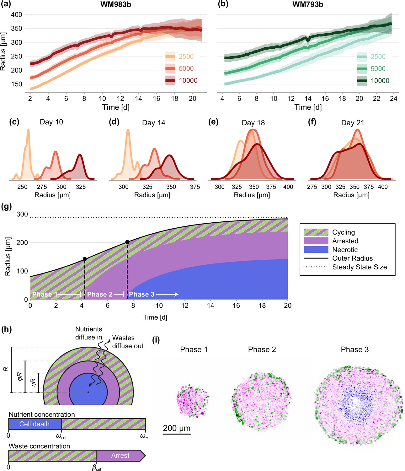
Experimental data and mathematical model.
(a–f) Growth of WM983b and WM793b spheroids over three weeks, initiated using approximately 2500, 5000 and 10,000 cells. The solid curve represents average outer radius and the coloured region corresponds to a 95% prediction interval (mean ± 1.96 std). (c–f) Size distribution of WM983b spheroids at days 10, 14, 18, and 21 for each initial seeding density. (g–h) Dynamics of the Greenspan, 1972 model, which describes three phases of growth and the development of a stable spheroid structure under assumptions of nutrient and waste diffusion. We denote by the spheroid radius, the relative radius of the arrested region and the relative radius of the necrotic core. (i) Optical sections showing three phases of growth in the experimental data (WM983b spheroids initiated with 2500 cells at days 3, 7, and 14). Colouring indicates cell nuclei positive for mKO2 (magenta), which indicates cells in gap 1; cell nuclei positive for mAG (green), which indicates cells in gap 2; and cell nuclei stained with DRAQ7 (blue), which indicates necrosis.
Figure 2

Late-time progression of WM983b spheroids, randomly sampled from the 10 spheroids imaged from each condition (additional images in Supplementary file 2).
Overlaid are the three boundaries identified by the image processing algorithm: the entire spheroid, the inhibited region and the necrotic region. Each image shows a 800 × 800 µm field of view. Colouring indicates cell nuclei positive for mKO2 (magenta), which indicates cells in gap 1; and cell nuclei positive for mAG (green), which indicates cells in gap 2.
Figure 3
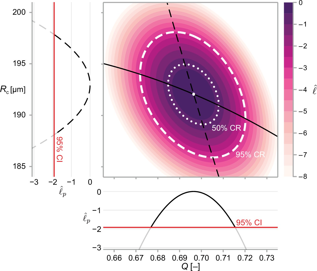
We calculate approximate confidence intervals (CI) using profile likelihood and confidence regions (CR) using contours of the normalised likelihood function.
Results demonstrate estimates of and using the structural model, Equation 6, and data from WM983b spheroids at day 14 initiated using 5000 cells. Point estimates are calculated using the maximum likelihood estimate (white marker). The boundaries of regions are defined as contours of the log-likelihood function. Univariate confidence intervals are constructed by profiling the log-likelihood and using a threshold of approximately −1.92 for a 95% confidence interval.
Figure 4
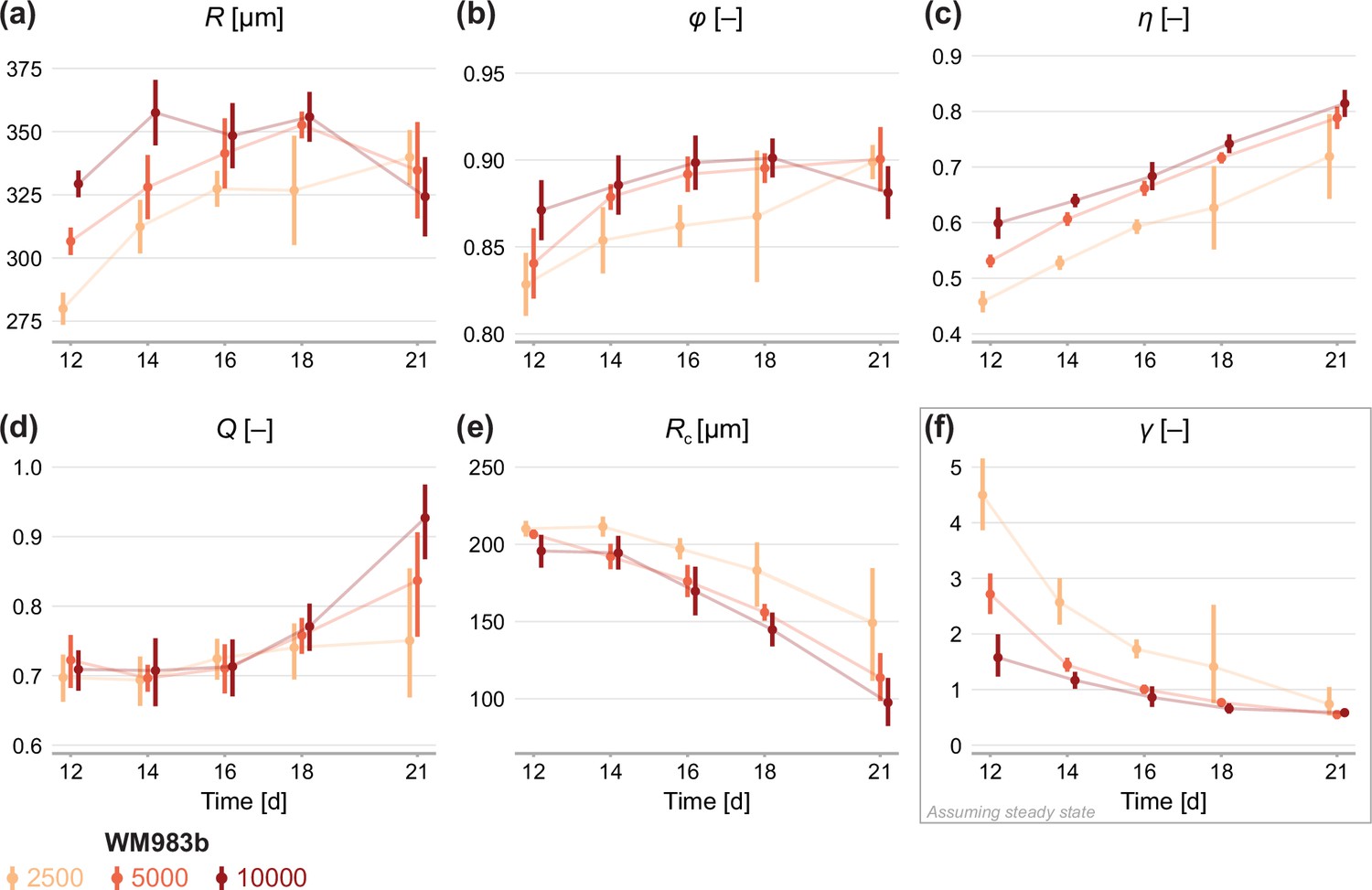
Estimates of parameters using the structural model with data from various time points.
In (a–c), parameters are the mean of each observation: . In (d–e), parameters are those in the structural model: . In (f), estimates of are obtained by calibrating observations to the steady-state model. As estimates and can be derived from the structural model (Equation 6), which applies at any time during phase 3, we expect to see similar parameter estimates across observation times. As estimates of can only be obtained from the steady-state model, which assumes the outer radius is no longer increasing, we do not expect to see similar parameter estimates across observation times. Bars indicate an approximate 95% confidence interval.
Figure 5
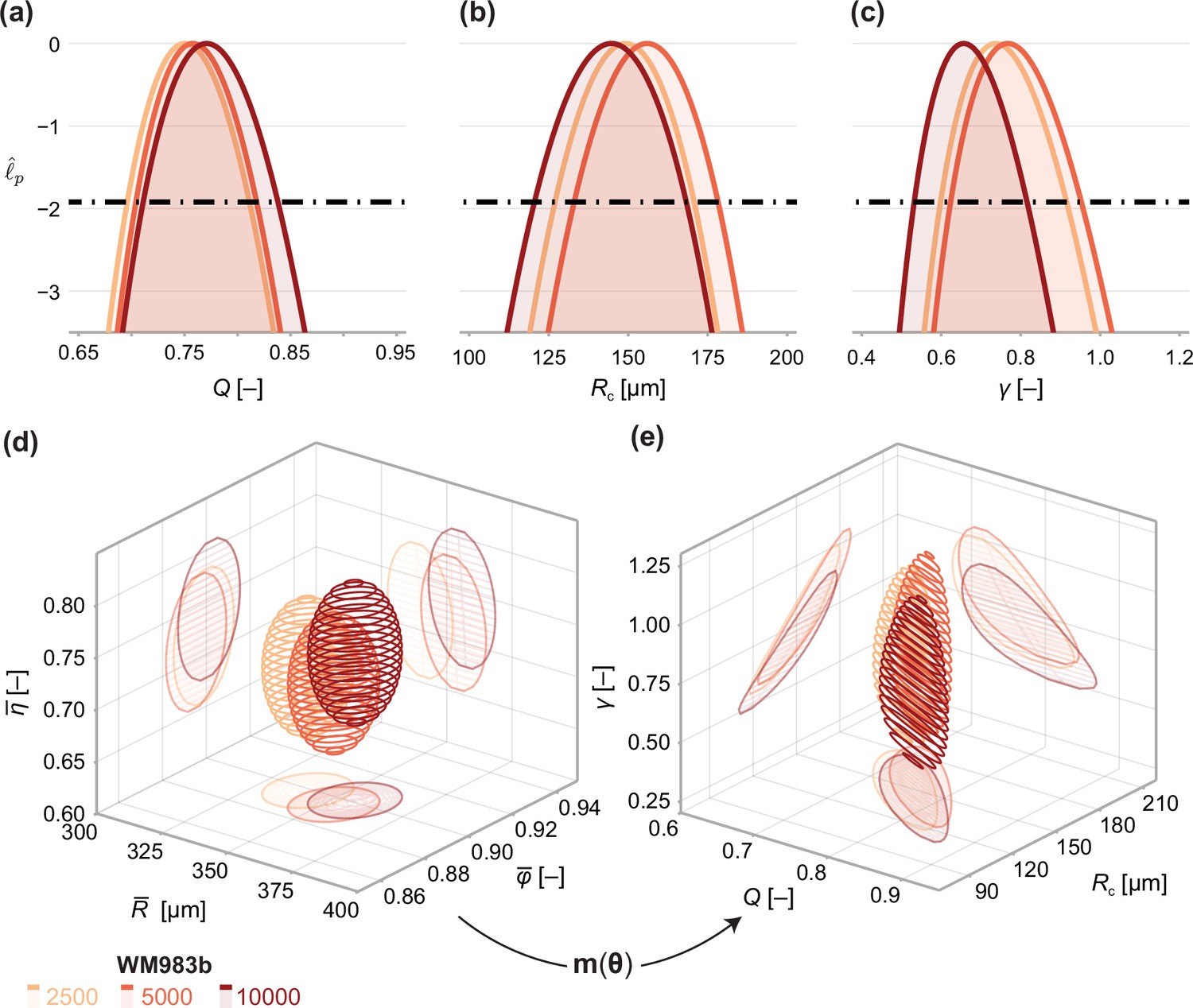
Comparison of WM983b spheroids between each initial seeding density at day 18 (spheroids seeded with 5000 or 10000 cells) and day 21 (2500).
(a–c) Profile likelihoods for each parameter, which are used to compute approximate confidence intervals (Table 1). (d) 95% confidence region for the full parameter space. 95% confidence regions for (d) the mean of each observation at steady state and (e) the model parameters .
Figure 6
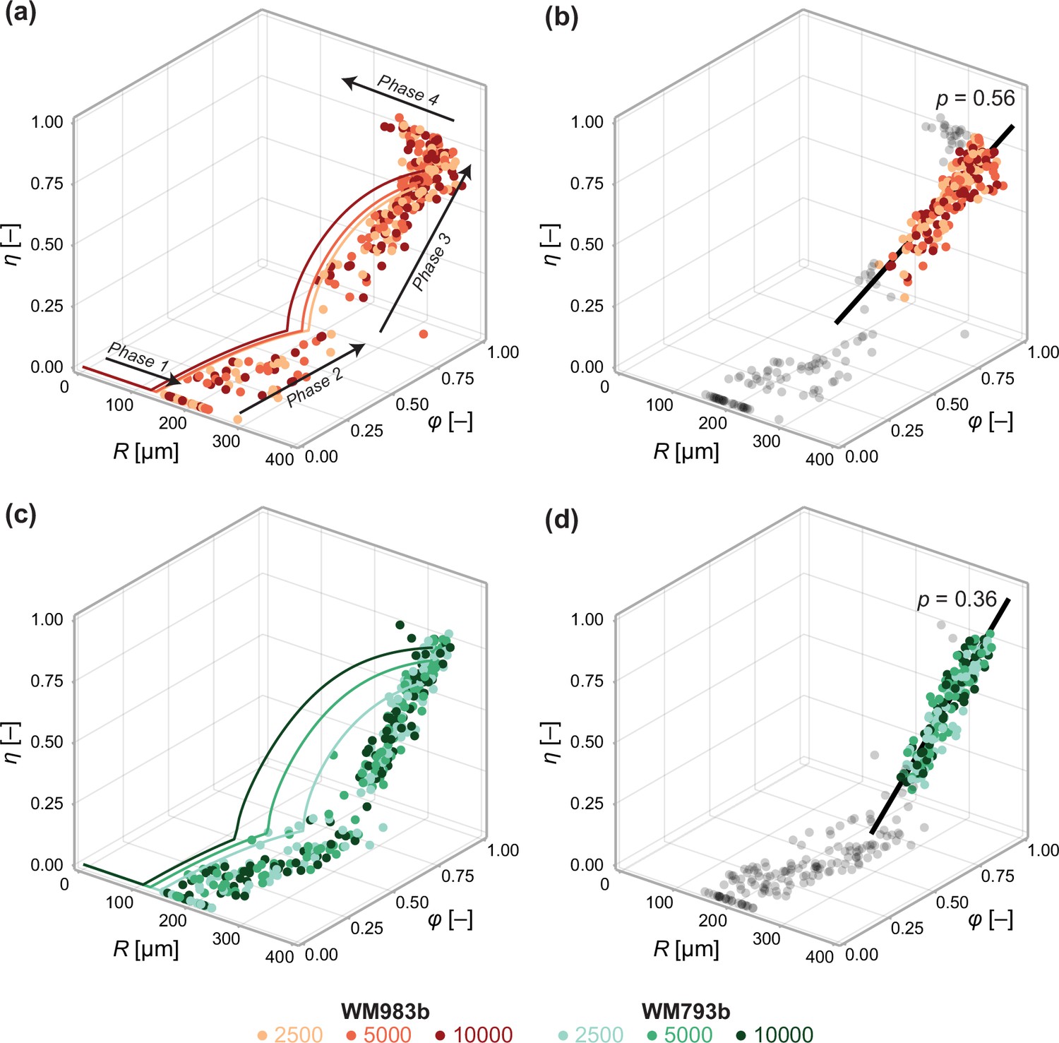
Data from days 3 to 21 (WM983b) and days 4 to 24 (WM793b) for all initial conditions.
Solid curves in (a) show the solution to the mathematical model (Equation 6) using the maximum likelihood estimate calculated using the steady-state data (Table 1). Solid curves in (c) show the solution to the mathematical model (Equation 6) using using the maximum likelihood estimate calculated using day 24 data. In (b) and (d), we fit a linear model to phase 3 data (indicated by coloured markers). The p value corresponds to a hypothesis test where the linear model parameters are the equivalent for all initial conditions. Shown in black is the best fit linear model.
Appendix 1—figure 1
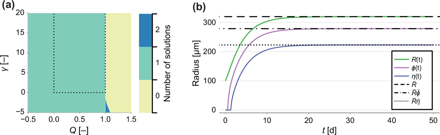
Number of solutions of Equation 20.
(a) Number of solutions to Equation 20 subject to the constraint 0 ≤ ρ ≤ 1. Dashed line indicates the region of interest, where γ > 0 and 0 < Q < 1. (b) Comparison between a long-term solution to the transient model and the semi-analytical solution to the steady state, where Q = 0.8, γ = 1, Rc = 150, s = 1 and R0 = 100.
Appendix 2—figure 1
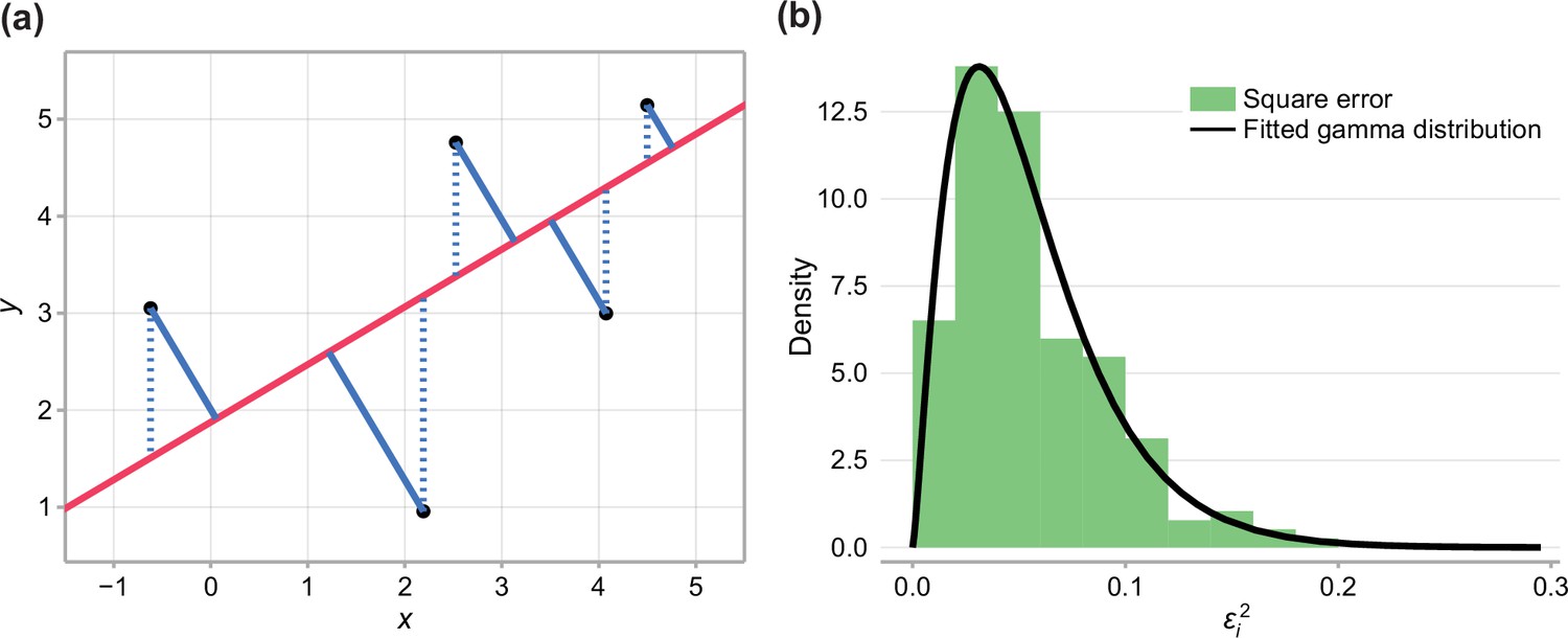
Fitting experimental data to linear model.
(a) Comparison between typical least-squares error (blue dashed), and total-least-squares error (blue solid). (b) Square error observed in the data and fitted gamma distribution.
Appendix 3—figure 1

Estimates of parameters using the structural model with data from various time points.
In (a–c), parameters are the mean of each observation: . In (d–e), parameters are those in the structural model: . In (f), estimates of are obtained by calibrating observations to the steady-state model. As estimates and can be derived from the structural model, which applies at any time during phase 3, we expect to see consistent estimates across observation times. Given that WM793b spheroids initiated with 2500 cells do not reach phase 3 until day 14, we exclude day 12 for these spheroids from the mathematical analysis. As estimates of can only be derived from the steady-state model, which assumes the outer radius is no longer increasing, we only expect consistency for later observation days. Bars indicate an approximate 95% confidence interval.
Tables
Table 1
Parameter estimates and approximate confidence intervals for each initial conditions.
Also shown are p-values for likelihood-ratio-based hypothesis tests for parameter equivalence between seeding densities.
| Parameter | θ2500 | θ5000 | θ10000 | p 2500,5000 | p 5000,10000 |
|---|---|---|---|---|---|
| 340.0 (331.0, 349.0) | 353.0 (344.0, 361.0) | 356.0 (347.0, 365.0) | 0.0420 | 0.617 | |
| 0.899 (0.889, 0.908) | 0.895 (0.886, 0.905) | 0.901 (0.891, 0.911) | 0.617 | 0.406 | |
| 0.719 (0.674, 0.764) | 0.716 (0.671, 0.761) | 0.742 (0.696, 0.788) | 0.940 | 0.438 | |
| μ | 0.202 | 0.687 | |||
| 0.75 (0.696, 0.811) | 0.758 (0.704, 0.818) | 0.771 (0.711, 0.838) | 0.854 | 0.767 | |
| 149.0 (127.0, 171.0) | 156.0 (133.0, 178.0) | 145.0 (121.0, 168.0) | 0.672 | 0.503 | |
| 0.737 (0.598, 0.916) | 0.768 (0.624, 0.953) | 0.657 (0.532, 0.816) | 0.792 | 0.308 | |
| 0.202 | 0.687 | ||||
Additional files
-
Transparent reporting form
- https://cdn.elifesciences.org/articles/73020/elife-73020-transrepform1-v2.docx
-
Supplementary file 1
Spheroid count per experimental condition (harvest day, seeding density and cell line).
- https://cdn.elifesciences.org/articles/73020/elife-73020-supp1-v2.docx
-
Supplementary file 2
Additional cross-sectional confocal images of spheroids; 10 per experimental condition (harvest day, seeding density and cell line).
- https://cdn.elifesciences.org/articles/73020/elife-73020-supp2-v2.pdf
-
Supplementary file 3
Reproduction of Figure 5 using data from day 21 for all initial seeding densities.
- https://cdn.elifesciences.org/articles/73020/elife-73020-supp3-v2.pdf
Download links
A two-part list of links to download the article, or parts of the article, in various formats.
Downloads (link to download the article as PDF)
Open citations (links to open the citations from this article in various online reference manager services)
Cite this article (links to download the citations from this article in formats compatible with various reference manager tools)
Quantitative analysis of tumour spheroid structure
eLife 10:e73020.
https://doi.org/10.7554/eLife.73020


