Modeling the spatiotemporal spread of beneficial alleles using ancient genomes

Version of Record

Accepted for publication after peer review and revision.

Download
Cite
Share
CommentOpen annotations (there are currently 0 annotations on this page).

Version of Record updated: December 21, 2022 (Go to version)
Version of Record published: December 20, 2022 (This version)
Accepted: November 21, 2022
Received: September 9, 2021
Preprint posted: July 22, 2021 (Go to version)

1. Of interest
The rapidly evolving X-linked MIR-506 family fine-tunes spermatogenesis to enhance sperm competition

Zhuqing Wang, Yue Wang ... Wei Yan

Research Article Apr 19, 2024
Further reading

Abstract
Editor's evaluation
Introduction
Results
Discussion
Methods
Appendix 1
Appendix 2
Data availability
References
Article and author information
Metrics

Abstract

Ancient genome sequencing technologies now provide the opportunity to study natural selection in unprecedented detail. Rather than making inferences from indirect footprints left by selection in present-day genomes, we can directly observe whether a given allele was present or absent in a particular region of the world at almost any period of human history within the last 10,000 years. Methods for studying selection using ancient genomes often rely on partitioning individuals into discrete time periods or regions of the world. However, a complete understanding of natural selection requires more nuanced statistical methods which can explicitly model allele frequency changes in a continuum across space and time. Here we introduce a method for inferring the spread of a beneficial allele across a landscape using two-dimensional partial differential equations. Unlike previous approaches, our framework can handle time-stamped ancient samples, as well as genotype likelihoods and pseudohaploid sequences from low-coverage genomes. We apply the method to a panel of published ancient West Eurasian genomes to produce dynamic maps showcasing the inferred spread of candidate beneficial alleles over time and space. We also provide estimates for the strength of selection and diffusion rate for each of these alleles. Finally, we highlight possible avenues of improvement for accurately tracing the spread of beneficial alleles in more complex scenarios.

Editor's evaluation

This is an important manuscript that presents an elegant framework to infer the dynamics of beneficial alleles over time and space. The authors present a new method and show, convincingly, its utility and great potential to reconstruct the evolutionary history of beneficial alleles. The method is also applied to loci that likely mediated human genetic adaptations, contributing to our understanding of human recent evolution. The work will be of broad interest to evolutionary biologists who seek to understand the dynamics of beneficial mutations in populations.

https://doi.org/10.7554/eLife.73767.sa0

Introduction

Understanding the dynamics of the spread of a beneficial allele through a population is one of the fundamental problems in population genetics (Ewens, 2012). We are often interested in knowing the location where an allele first arose and the way in which it spread through a population, but this is often unknown, particularly in natural, non-experimental settings where genetic sampling is scarce and uneven.

Patterns of genetic variation can be used to estimate how strongly natural selection has affected the trajectory of an allele and to fit the parameters of the selection process. The problem of estimating the age of a beneficial allele, for example, has yielded a rich methodological literature (Slatkin and Rannala, 2000), and recent methods have exploited fine-scale haplotype information to produce highly accurate age estimates (Mathieson and McVean, 2014; Platt et al., 2019; Albers and McVean, 2020). In contrast, efforts to infer the geographic origins of beneficial mutations are scarcer. These include Novembre et al., 2005, who developed a maximum likelihood method to model the origin and spread of a beneficial mutation and applied it to the CCR5-Δ32 allele, which was, at the time, considered to have been under positive selection (Stephens et al., 1998; Sabeti et al., 2005; Novembre and Han, 2012). Similarly, Itan et al., 2009 developed an approximate Bayesian computation (ABC) approach using demic simulations, in order to find the geographic and temporal origins of a beneficial allele, based on present-day allele frequency patterns.

As ancient genome sequences become more readily available, they are increasingly being used to understand the process of natural selection (see reviews in Malaspinas et al., 2012; Dehasque et al., 2020). However, few studies have used ancient genomes to fit spatial dynamic models of the spread of an allele over a landscape. Most spatiotemporal analyses that included ancient genomes have used descriptive modeling in order to learn the spatiotemporal covariance structure of allele frequencies (Segurel et al., 2020) or hidden ancestry clusters (Racimo et al., 2020b), and then used that structure to hindcast these patterns onto a continuous temporally evolving landscape. In contrast to descriptive approaches, dynamic models have the power to infer interpretable parameters from genomic data and perhaps reveal the ultimate causes for these patterns (Wikle et al., 2019).

Dynamic models can also contribute to ongoing debates about the past trajectories of phenotypically important loci. For example, the geographic origin of the rs4988235(T) allele—upstream of the LCT gene and associated with adult lactase persistence in most of Western Eurasia (Enattah et al., 2002)—remains elusive, as is the way in which it spread (an extensive review can be found in Ségurel and Bon, 2017). The allele has been found in different populations, with frequencies ranging from 5% up to almost 100%, and its selection coefficient has been estimated to be among the highest in human populations (Bersaglieri et al., 2004; Enattah et al., 2008; Tishkoff et al., 2007). However, the exact causes for its adaptive advantage are contested (Szpak et al., 2019), and it has been suggested that the selection pressures acting on the allele may have been different in different parts of the continent (Gerbault et al., 2009). Ancient DNA evidence shows that the allele was rare in Europe during the Neolithic (Burger et al., 2007; Gamba et al., 2014; Allentoft et al., 2015; Mathieson et al., 2015) and only became common in Northern Europe after the Iron Age, suggesting a rise in frequency during this period, perhaps mediated by gene flow from regions east of the Baltic where this allele was more common during the onset of the Bronze Age (Krüttli et al., 2014; Margaryan et al., 2020). Itan et al., 2009 deployed their ABC approach to model the spatial spread of the rs4988235(T) allele and estimated that it was first under selection among farmers around 7500 years ago possibly between the Central Balkans and Central Europe. Others have postulated a steppe origin for the allele (Allentoft et al., 2015), given that the rise in frequency appears to have occurred during and after the Bronze Age migration of steppe peoples into Western Eurasia (Haak et al., 2015; Allentoft et al., 2015). However, the allele is at low frequency in genomes of Bronze Age individuals associated with Corded Ware and Bell Beaker assemblages in Central Europe who have high steppe ancestry (Mathieson et al., 2015; Margaryan et al., 2020), complicating the story further (Ségurel and Bon, 2017).

The origins and spread dynamics of large-effect pigmentation-associated SNPs in ancient Eurasians have also been intensely studied (Ju and Mathieson, 2020). Major loci of large effect on skin, eye, and hair pigmentation have been documented as having been under recent positive selection in Western Eurasian history (Voight et al., 2006; Sabeti et al., 2007; Pickrell et al., 2009; Lao et al., 2007; Mathieson et al., 2015; Alonso et al., 2008; Hudjashov et al., 2013). These include genes SLC45A2, OCA2, HERC2, SLC24A5, and TYR. While there is extensive evidence supporting the adaptive significance of these alleles, debates around their exact origins and spread are largely driven by comparisons of allele frequency estimates in population groups, which are almost always discretized in time and/or space. Among these, selection at the TYR locus is thought to have occurred particularly recently, over the last 5000 years (Stern et al., 2019), driven by a recent mutation (Albers and McVean, 2020) that may have spread rapidly in Western Eurasia.

Here, we develop a method to model the spread of a recently selected allele across both space and time, avoiding artificial discretization schemes to more rigorously assess the evidence for or against a particular dispersal process. We begin with the model proposed by Novembre et al., 2005 and adapt it in order to handle ancient low-coverage genomic data and explore more complex models that allow for both diffusion and advection (i.e., directional transport) in the distribution of allele frequencies over space, as well as for a change in these parameters at different periods of time. We apply the method to alleles in two of the aforementioned loci in the human genome, which have been reported to have strong evidence for recent positive selection: LCT/MCM6 and TYR. We focus on Western Eurasia during the Holocene, where ancient genomes are most densely sampled, and infer parameters relevant to the spread of these alleles, including selection, diffusion and advection coefficients.

Results

Summary of model

We based our statistical inference framework on a model proposed by Novembre et al., 2005 to fit allele frequencies in two dimensions to present-day genotype data spread over a densely sampled map. We extend this model in several ways:

We incorporate temporally sampled data (ancient genomes) to better resolve changes in frequency distributions over time.
We make use of genotype likelihoods and pseudohaploid genotypes to incorporate low-coverage data into the inference framework.
We permit more general dynamics by including advection parameters.
We allow the selection, advection, and diffusion parameters to be different in different periods of time. Specifically, to reflect changes in population dynamics and mobility before and after the Bronze Age (Loog et al., 2017; Racimo et al., 2020a), we partitioned the model fit into two time periods: before and after 5000 years BP.

We explored the performance of two different spread models, which are extensions of the original model by Novembre et al., 2005, hereby called model A. This is a diffusion model containing a selection coefficient $s$ (determining the rate of local allele frequency growth) and a single diffusion term ( $σ$ ). A more general diffusion model—hereby model B—allows for two distinct diffusion parameters for latitudinal ( $σ_{y}$ ) and longitudinal ( $σ_{x}$ ) spread. Finally, model C is even more general and includes two advection terms (v_x and v_y), allowing the center of mass of the allele’s frequency to diverge from its origin over time. The incorporation of advection is meant to account for the fact that population displacements and expansions could have led to allele frequency dynamics that are poorly explained by diffusion alone.

In order to establish a starting time point for our diffusion process, we used previously published allele age estimates obtained from a nonparametric approach leveraging the patterns of haplotype concordance and discordance around the mutation of interest (Albers and McVean, 2020). In the case of the allele in the LCT/MCM6 region, we also used age estimates based on an approximate Bayesian computation approach (Itan et al., 2009).

Performance on deterministic simulations

To characterize the accuracy of our inference method under different parameter choices, we first generated deterministic simulations from several types of diffusion models. First, we produced an allele frequency surface map with a specified set of parameters from which we drew 1040 samples matching the ages, locations, and genotype calling format (diploid vs. pseudohaploid) of the 1040 genomes that we analyze below when studying the rs1042602(A) allele.

We generated six different simulations with different diffusion coefficients and afterward ran our method assuming model B. The results (simulations B1−B6) are summarized in Figure 1, Figure 1—figure supplements 1–5, and Appendix 2—table 1. Overall, the model is more accurate at correctly inferring the parameters for the time period before 5000 years BP (Figure 1b), with decreased performance when longitudinal diffusion is high (Figure 1—figure supplement 5).

Figure 1 with 7 supplements see all

Download asset Open asset

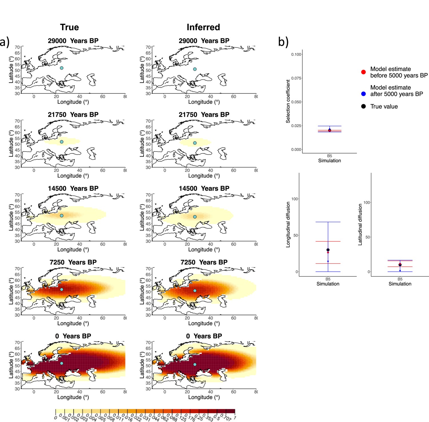
Comparison of true and inferred allele frequency dynamics for simulation B5.

(a) Comparison of true and inferred allele frequency dynamics for a simulation with diffusion and no advection (B5). The green dot corresponds to the origin of the allele. The parameter values used to generate the frequency surface maps are summarized in Appendix 2—table 1. (b) Comparison of true parameter values and model estimates. Whiskers represent 95% confidence intervals.

Next, we investigated the performance of model C, which includes advection coefficients. We generated four different simulations including advection (simulations C1−C4: Figure 2, Figure 1—figure supplements 1–3, and Appendix 2—table 2). We found that our method is generally able to estimate the selection coefficient accurately. However, in some of the simulations, we found discrepancies between the estimated and true diffusion and advection coefficients, often occurring because of a misestimated origin forcing the other parameters to adjust in order to better fit the allele frequency distribution in later stages of the allele’s spread (Figure 2). Despite the disparities between the true and inferred parameter values, the resulting surface plots become very similar as we approach the present, suggesting that different combinations of parameters can produce similar present-day allele frequency distributions.

Figure 2 with 3 supplements see all

Download asset Open asset

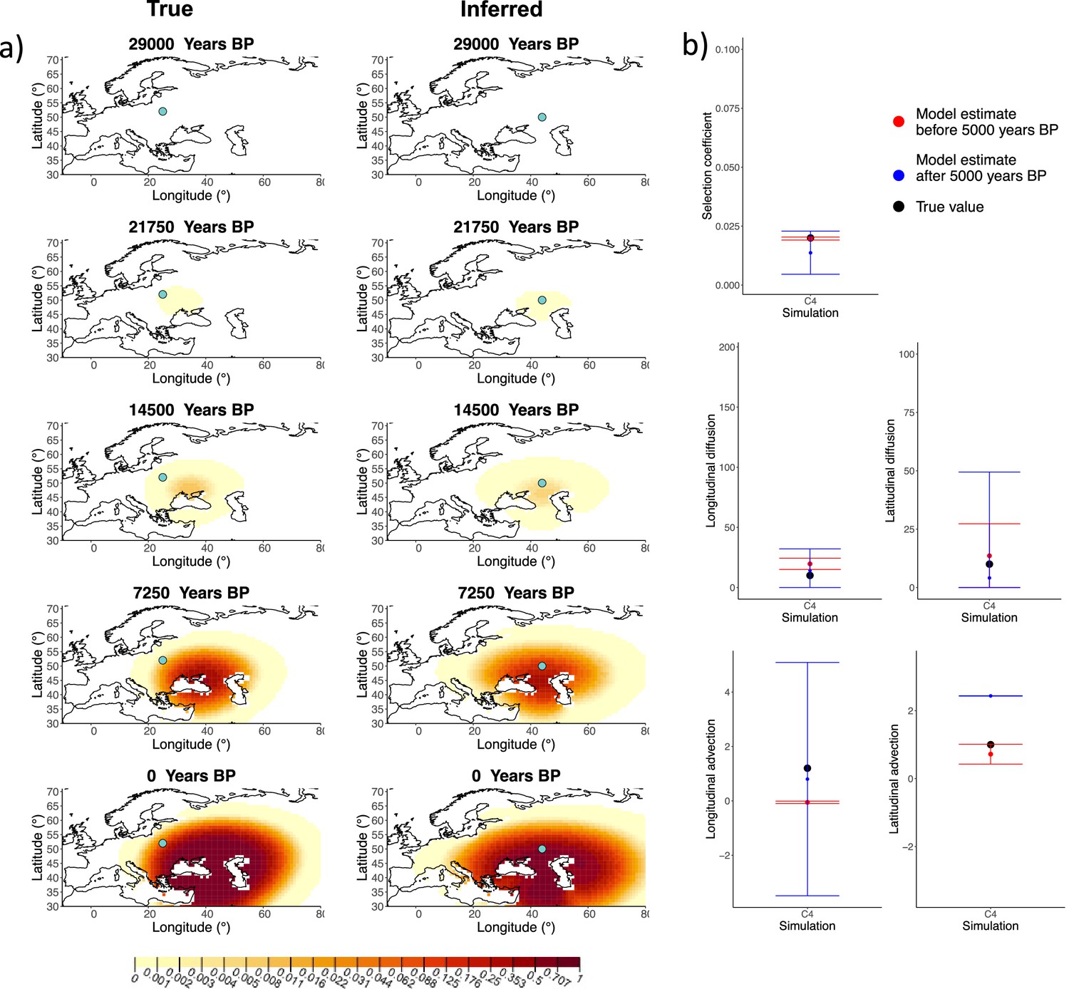
Comparison of true and inferred allele frequency dynamics for simulation C4.

(a) Comparison of true and inferred allele frequency dynamics for one of the simulations including advection (C4). The green dot corresponds to the origin of the allele. The parameter values used to generate the frequency surface maps are summarized in Appendix 2—table 2. (b) Comparison of true parameter values and model estimates. Whiskers represent 95% confidence intervals.

Advection model applied to non-advection simulations

We assessed model performance when we apply model C, which includes advection coefficient estimates, to simulations generated without advection (see Figure 1—figure supplements 6 and 7). We can observe that the advection coefficients are inferred to be non-zero (Figure 1—figure supplements 6b and 7b); however, the inferred allele frequency dynamic plots closely resemble the ones obtained with true parameter values (Figure 1—figure supplements 6a and 7a). This shows that complex interactions between the diffusion and advection coefficients can result in similar outcomes even when only diffusion is considered in the model.

The inference of the origin of the allele also differs when we compare results when using models B and C. In order to understand better how the model estimates the allele origin, we highlighted the first individual in simulations B1 and B4 that contains the derived allele. We can see that in the case of simulation B1 the inferred origin of the allele is close to the first observance of the derived allele in the model that includes advection. In contrast when the advection is not included, the origin of the allele is inferred to be closer to where it is initially rising in frequency (Figure 1—figure supplements 1a and 4a). However, this is not always the case. For instance, if we look at the results from the advection model on simulation B4, we can see that the origin of the allele is inferred relatively far from the sample known to have carried the first instance of the derived allele. Therefore, if there is a relatively large interval between the time when the allele originated and when the first ancient genomes are available, the beneficial allele can spread widely, but as this spread is not captured by any of the data points, inference of the precise origin of the selected allele is nearly impossible.

Impact of sample clustering on parameter estimates

We evaluated the impact of different sampling and clustering schemes on our inferences that could potentially arise by aggregating aDNA data from studies with different sampling schemes. We used a deterministic simulation to create three different degrees of clustering, which we will refer to as ‘homogeneous,’ ‘intermediate,’ or ‘extreme’ by varying the area from which we sample individuals to be used in our inferences (Figure 3—figure supplement 1). Additionally, we also tested the impact of biased temporal sampling in the periods before and after 5000 years BP by oversampling in the ancient period (75%/25%), equally sampling in the two periods (50%/50%), and oversampling in the recent period (25%/75%). Because we evaluated this temporal bias for each of the three spatial clustering sampling scenarios, this resulted in a total of nine different sampling scenarios. We note that the third ‘extreme’ spatial clustering scenario is completely unrealistic and one would not expect inferences of any degree of accuracy from it, but we believe it gives a good idea of the behavior of our method in the limiting case of extremely restricted spatial sampling.

A comparison of allele frequency maps generated using true parameter values and using parameter estimates from the different sampling schemes is shown in Figure 3—figure supplements 2–9. In Figure 3 we show the allele frequency map generated using the ‘intermediate 75%/25%’ clustering scheme. Parameter estimates used to generate all these figures are summarized in Appendix 2—table 3. Overall we can see that the allele frequency maps inferred from these scenarios closely resemble the maps generated using the true parameter values, despite the challenges in finding accurate values for the individual point estimates of some of the parameters, highlighting that various combinations of diffusion and advection coefficients can produce similar underlying frequency maps (as discussed in the section ‘Performance on deterministic simulations’). This suggests that the joint spatiotemporal information encoded in the inferred maps (not just the individual parameters estimates) should be used in interpreting model outputs, particularly when it comes to the advection and diffusion parameters. The selection coefficient estimates are inferred highly accurately, regardless of the sampling scheme chosen, and lie close to the true value, with only a slight underestimation in the time period after 5000 years BP (with the exception of the ‘extreme 25%/75%’).

Figure 3 with 9 supplements see all

Download asset Open asset

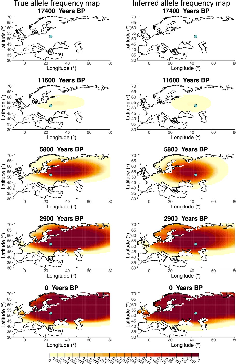
Comparison of true allele frequency map and map generated using ‘intermediate 75%/25%’ clustering scheme.

Left: allele frequency map generated using true parameter values. Right: allele frequency map generated using parameter estimates for ‘intermediate 75%/25%’ clustering scheme. Parameter values used to generate the maps are summarized in Appendix 2—table 3.

Spatially explicit forward simulations

In addition to drawing simulated samples from a diffusion model, we used SLiM (Haller and Messer, 2019) to perform spatially explicit individual-based forward-in-time simulations of selection acting on a beneficial allele by leveraging an R interface for spatial population genetics now implemented in the R package slendr (Petr, 2021).

We introduced a single beneficial additive mutation in a single individual and let it evolve across the European landscape. Before applying our method on the simulated data, we sampled 1040 individuals whose ages were log-uniformly distributed to ensure that there were more samples closer to the present, as in the real data. We transformed the diploid genotypes to pseudohaploid genotypes by assigning a heterozygous individual an equal probability of carrying the ancestral or the derived genotype. The parameter values estimated by our model to the simulations described in this section are summarized in Appendix 2—table 4.

We can see that the origin of the allele inferred by the model closely corresponds to the first observation of the derived allele in the simulation (Figure 4). The inferred selection coefficient is only slightly higher than the true value from the simulation (0.0366 vs. 0.030). In general, the model accurately captures the spread of the allele centered in Central Europe, though we observe some discrepancies due to differences between the model assumed in the simulation (which, e.g., accounts for local clustering of individuals, Figure 4—figure supplement 1), and that assumed by our diffusion-based inference.

Figure 4 with 1 supplement see all

Download asset Open asset

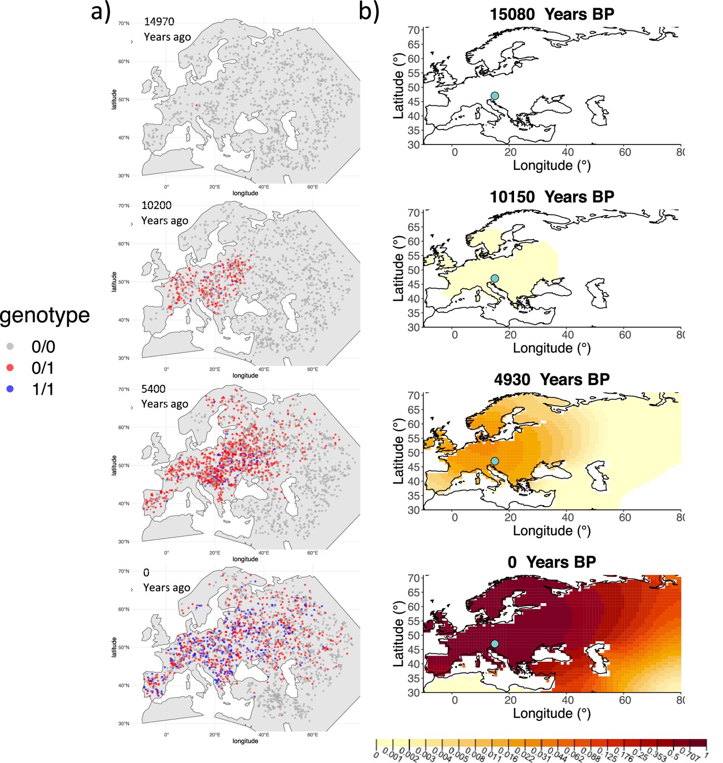
Comparison of an individual-based simulation and allele frequency dynamics inferred by the diffusion model.

(A) Individual-based simulation of an allele that arose in Central Europe 15,000 years ago with a selection coefficient of 0.03. Each dot represents a genotype from a simulated genome. To avoid overplotting, only 1000 out of the total 20,000 individuals in the simulation in each time point are shown for each genotype category. (B) Allele frequency dynamics inferred by the diffusion model on the individual-based simulation to the left, after randomly sampling 1040 individuals from the simulation and performing pseudohaploid genotype sampling on them. The ages of sampled individuals were log-uniformly distributed. The estimated parameter values of the fitted model are shown in Appendix 2—table 4.

Dynamics of the rs4988235(T) allele

Having tested the performance of our method on simulated data, we set out to infer the allele frequency dynamics of the rs4988235(T) allele (associated with adult lactase persistence) in ancient Western Eurasia. For our analysis, we used a genotype dataset compiled by Segurel et al., 2020, which amounts to 1434 genotypes from ancient Eurasian genomes individuals, and a set of 36,659 genotypes from present-day Western and Central Eurasian genomes (Ségurel and Bon, 2017; Heyer et al., 2011; Marchi et al., 2018; Liebert et al., 2017; Gallego Romero et al., 2012; Itan et al., 2010; Charati et al., 2019). After filtering out individuals falling outside of the range of the geographic boundaries considered in this study, we retained 1332 ancient individuals. The locations of ancient and present-day individuals used in the analysis to trace the spread of rs4988235(T) are shown in Figure 5.

Figure 5

Download asset Open asset

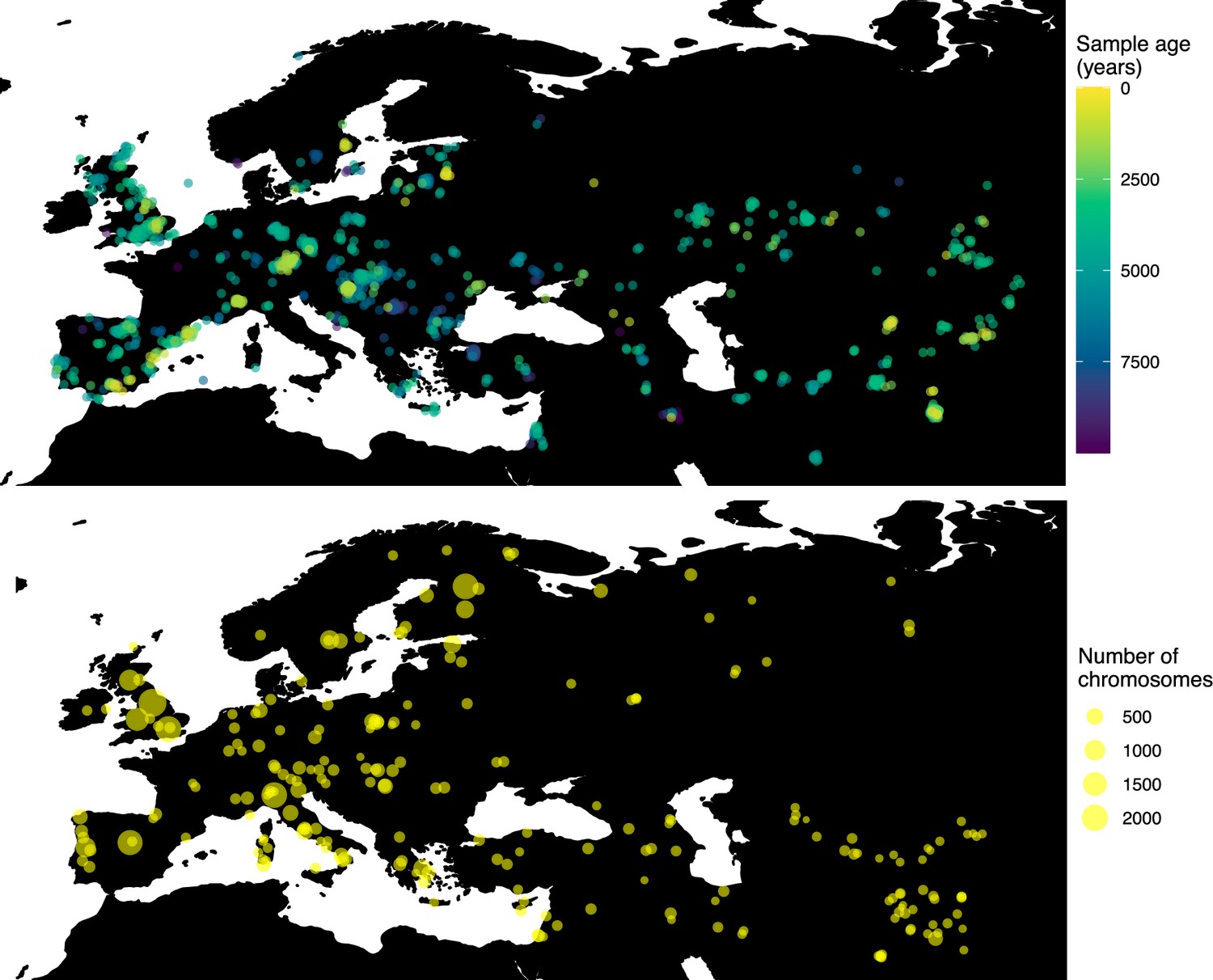
Locations of samples used to model the spread of the rs4988235(T) allele.

The upper panel shows the spatiotemporal locations of ancient individuals, and the bottom panel represents the locations of present-day individuals.

We used a two-period scheme by allowing the model to have two sets of estimates for the selection coefficient and the diffusion and advection coefficients in two different periods of time: before and after 5000 years ago, reflecting the change in population dynamics and mobility before and after the Bronze Age transition (Loog et al., 2017; Racimo et al., 2020a). We used two allele age estimates as input: a relatively young one (7441 years ago) obtained by using the estimated start of selection onset from Itan et al., 2009 (though we note this is necessarily a lower bound of the age of mutation origin), and a relatively old one (20,106 years ago) obtained from the age estimate from Albers and McVean, 2020. The results obtained for fitting the model on rs4988235(T) are summarized in Appendix 2—table 5 and Appendix 2—table 6, and in Figure 6b (younger age) and Figure 6—figure supplement 1 (older age).

Figure 6 with 9 supplements see all

Download asset Open asset

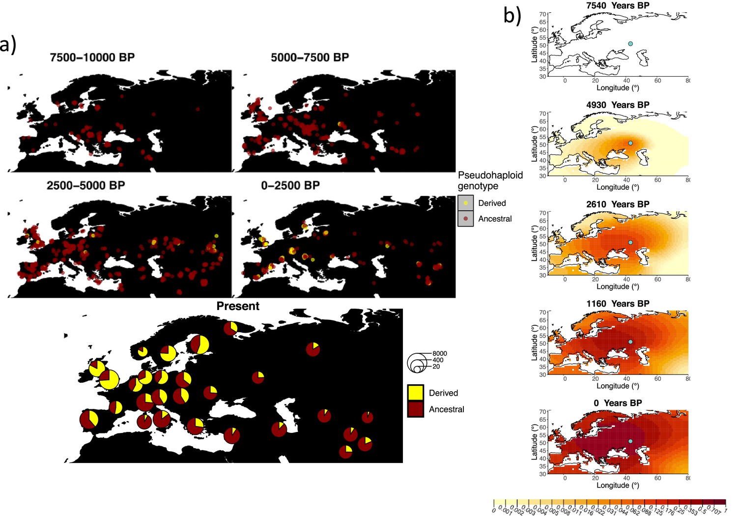
Allele frequency dynamics of rs4988235(T).

(a) Top: pseudohaploid genotypes of ancient samples at the rs4988235 SNP in different periods. Yellow corresponds to the rs4988235(T) allele. Bottom: allele frequencies of present-day samples represented as pie charts. The size of the pie charts corresponds to the number of available sequences in each region. (b) Inferred allele frequency dynamics of rs4988235(T). The green dot indicates the inferred geographic origin of the allele.

Assuming the mutation age estimate is equivalent to the start of selection onset from Itan et al., 2009, the origin of the allele is estimated to be north of the Caucasus, around what is now southwestern Russia and eastern Ukraine (Figure 6b). Given that this age is relatively young, our method fits a very strong selection coefficient ( $\approx 0.1$ ) during the first period in order to accommodate the early presence of the allele in various points throughout Eastern Europe, and a weaker (but still strong) selection coefficient ( $\approx 0.03$ ) in the second period. We also estimate stronger diffusion in the second period than in the first, to accommodate the rapid expansion of the allele throughout Western Europe, and a net westward advection parameter, indicating movement of the allele frequency’s center of mass to the west as we approach the present.

Assuming the older age estimate from Albers and McVean, 2020, the origin of the allele is estimated to be in the northeast of Europe (Figure 6—figure supplement 1), which is at a much higher latitude than the first occurrence of the allele, in Ukraine. Due to the deterministic nature of the model, the frequency is implicitly imposed to expand in a region where there are no actual observed instances of the allele. The model compensates for this by placing the origin in an area with a lower density of available aDNA data and thus avoiding an overlap of the increasing allele frequencies with individuals who do not carry the derived rs4988235(T) allele (see Figure 6a). As the model expands rapidly in the southern direction (Appendix 2—table 6) it eventually reaches the sample carrying the derived variant in Ukraine.

Dynamics of the rs1042602(A) allele

Next, we investigated the spatiotemporal dynamics of the spread of an allele at a pigmentation-associated SNP in the TYR locus (rs1042602(A)), which has been reported to be under recent selection in Western Eurasian history (Stern et al., 2019). For this purpose, we applied our method to the Allen Ancient DNA Resource data (Reich and Mallick, 2019), which contains randomly sampled pseudohaploid genotypes from 1513 published ancient Eurasian genomes (listed in Supplementary file 1), from which we extracted those that had genotype information at this locus in Western Eurasia. We merged this dataset with diploid genotype information from high-coverage present-day West Eurasian genomes from the Human Genome Diversity Panel (HGDP) (Bergström et al., 2020), which resulted in a total of 1040 individuals with genotype information at rs1042602, which were used as input to our analysis. Geographic locations of individuals in the final dataset are shown in Figure 7.

Figure 7

Download asset Open asset

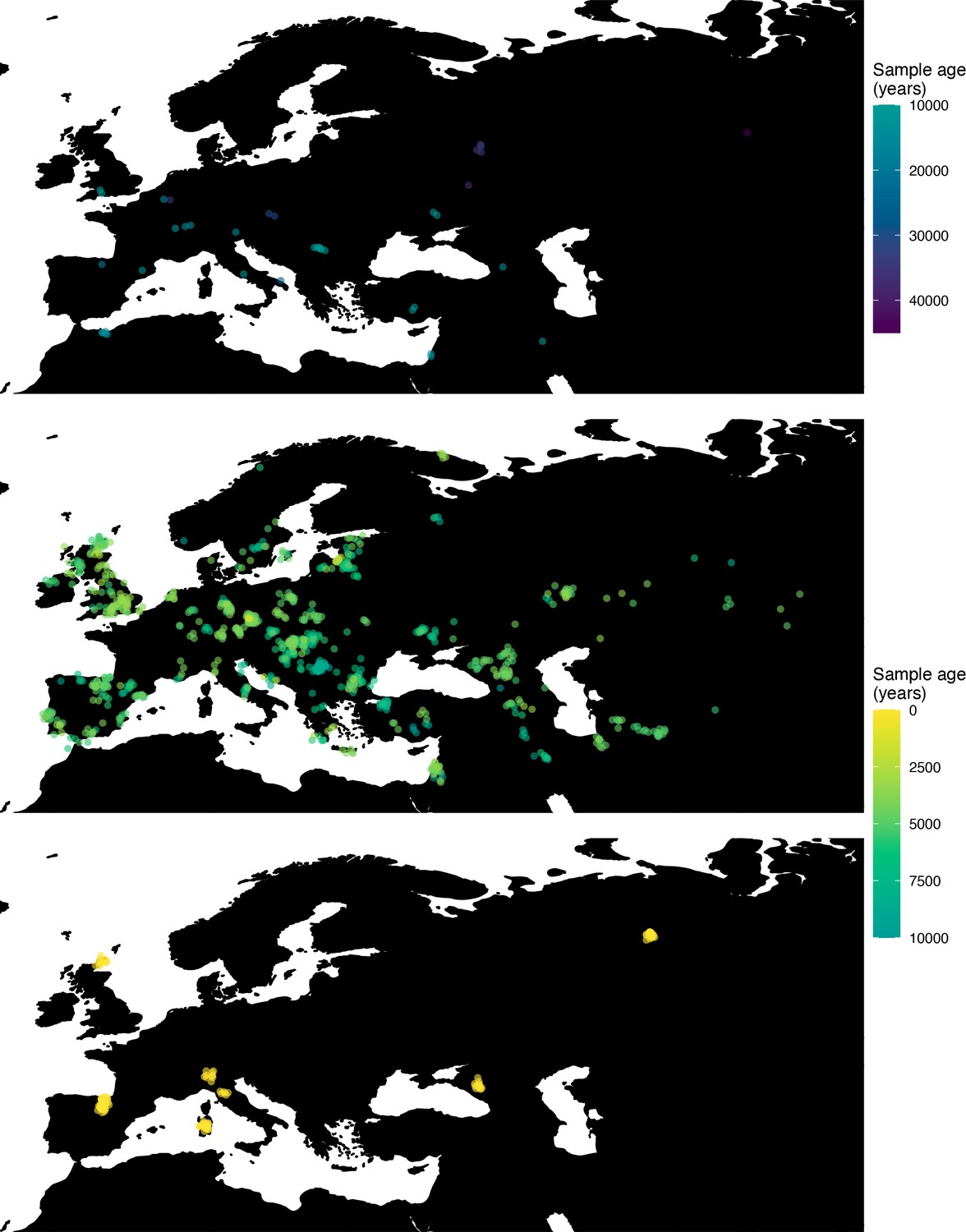
Spatiotemporal sampling locations of sequences used to model the rs1042602(A) allele in Western Eurasia.

Upper panel: ancient individuals dated as older than 10,000 years ago. Middle panel: ancient individuals dated as younger than 10,000 years ago. Bottom panel: present-day individuals from the Human Genome Diversity Panel (HGDP).

Similarly to our analysis of the spread of the allele in rs4988235(T), we inferred the dynamics of the rs1042602(A) allele separately for the time periods before and after 5000 years BP and assuming the age of the allele to be 26,361 years (Albers and McVean, 2020). The inferred parameters for both time periods are summarized in Appendix 2—table 7, and the allele frequency surface maps generated using these parameters are shown in Figure 8b. The origin of the rs1042602(A) corresponds closely to the region where the allele initially starts to segregate in the time period between 7500 and 10,000 years BP as seen in Figure 8a. Estimates of the selection coefficient for both time periods (0.0221 and 0.0102 for the period before and after 5000 years BP, respectively) suggest that selection acting on the allele has decreased after 5000 years BP.

Figure 8 with 6 supplements see all

Download asset Open asset

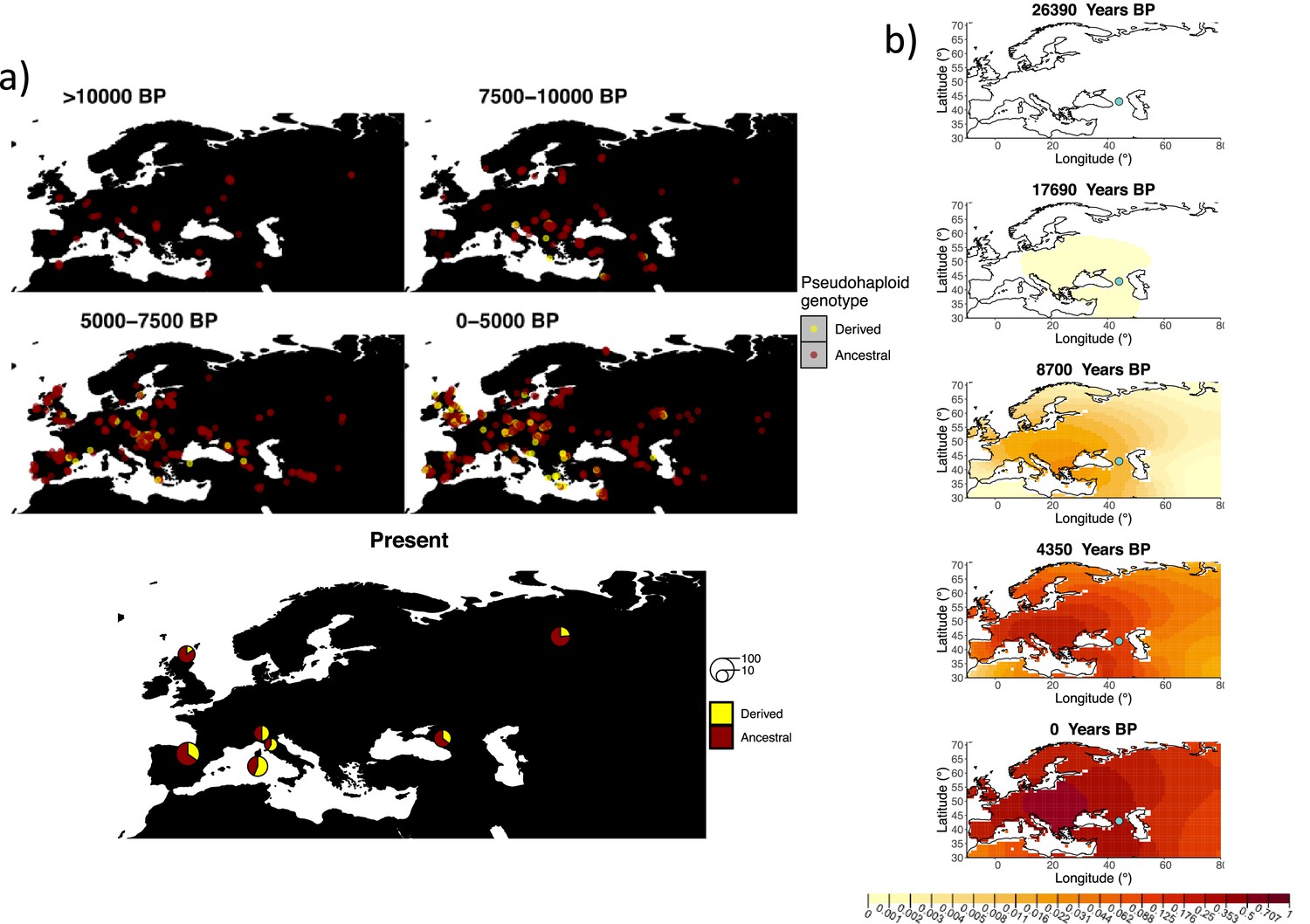
Allele frequency dynamics of rs1042602(A).

(a) Top: pseudohaploid genotypes of ancient samples of the rs1042602 in different periods. Yellow corresponds to the A allele. Bottom: diploid genotypes of present-day samples. (b) Inferred allele frequency dynamics of rs1042602(A). The green dot corresponds to the inferred geographic origin of the allele.

Robustness of parameters to the inferred geographic origin of allele

We carried out an analysis to characterize how sensitive the selection, diffusion, and advection parameters are to changes in the assumed geographic origin of the allele. For the rs4988235(T) allele, we forced the origin of the allele to be 10° away from our inferred origin in each cardinal direction, while assuming the allele age is equal to the inferred start of selection onset from Itan et al., 2009 (Appendix 2—table 8). In Figure 6—figure supplements 2–5, we can see the allele frequency dynamics of these four scenarios, respectively. We also forced the allele origin to be at the geographic origin estimated in Itan et al., 2009 (Figure 6—figure supplement 6, Appendix 2—table 9), which is westward of our estimate. In all five cases during the period prior 5000 years BP, the allele is inferred to expand in the direction of the first sample that is observed to carry the rs4988235(T) allele and is located in Ukraine. During the time period after 5000 years BP, the patterns produced by the model are rather similar, although the parameters associated with diffusion and advection differ, in order to account for the different starting conditions.

We also investigated how the results are affected when the estimated geographic origin of the rs1042602(A) allele is moved with respect to the initial estimate. We set the allele to be 10° east, 10° north, and 10° south of the original estimate as shown in Figure 8—figure supplements 1–3, respectively (for parameter estimates see Appendix 2—table 10). We did not look at a scenario in which the origin of the allele is moved to the west since it would either end up in the Black Sea or more westward than 10°. The selection coefficient remains similar to the original estimate throughout all three scenarios. The way the allele spreads across the landscape is also similar in all cases and, as in the case of rs4988235(T), the model accounts for the different origins of the allele by adjusting the diffusion and advection coefficients in the time period after 5000 years BP.

Robustness of parameters to the assumed age of the allele

In order to investigate how sensitive our inferences are to the point estimates of allele ages we obtained from the literature (Albers and McVean, 2020; Itan et al., 2009), we also fitted our model using the upper and lower ends of the 95% confidence intervals or credible intervals for each age estimate (depending on whether the inference procedure in the literature was via a maximum likelihood or a Bayesian approach). For the rs4988235(T) allele, the reported credible intervals for the (Itan et al., 2009) age are 8683 and 6256 years BP. For the rs1042602(A) allele, the reported confidence intervals for the age are 27,315 and 25,424 years BP (Albers and McVean, 2020).

When refitting the model for the rs4988235(T) allele, we found that the inferred selection coefficient is slightly lower when the allele age is assumed to be at the lower bound of the 95% credible interval (0.0867 vs. 0.0993 before 5000 years BP and 0.0321 vs. 0.0328 after 5000 years BP) and slightly higher when assumed to be at the upper bound (0.0994 vs. 0.0993 before 5000 years BP and 0.0572 vs. 0.0328 after 5000 years BP) (Appendix 2—table 5 and Figure 6—figure supplements 7 and 8). This occurs because the selection intensity must be higher or lower when there is more or less time, respectively, for the allele to reach the allele frequencies observed in the data. In the case of the rs1042602(A) allele, this only affects the earlier time period (Appendix 2—table 7). The rs4988235(T) allele’s geographic distribution in the more recent time periods is also less extended geographically when the age is assumed to be young. The inferred geographic origin of both alleles slightly differs under different assumed ages (Figure 8—figure supplements 4 and 5).

In addition, we assessed the likelihood of the best-fitted models with varying the ages of the rs4988235(T) and rs1042602(A) alleles (Figure 6—figure supplement 9 and Figure 8—figure supplement 6, respectively). We can see that in the case of rs4988235(T) allele the allele age used in this study (7441 years) gives the most likely solution among the explored ages. In case of the rs1042602(A) allele, we found that there are multiple nearly equally likely ages when looking at ages at least as old as 15,000 years.

Discussion

A spatially explicit framework for allele frequency diffusion can provide new insights into the dynamics of selected variants across a landscape. We have shown that under the conditions of strong, recent selection, our method can infer selection and dispersal parameters using a combination of ancient and present-day human genomic data. However, when allowing for advection, the inferred location tends to become less accurate. This suggests that migration events early in the dispersal of the selected allele could create difficulties in finding the true allele origin if net directional movement (i.e., via major migratory processes) had a large effect in this dispersal. This issue could be alleviated with the inclusion of more ancient genomes around the time of the origin of the mutation, perhaps in combination with a more fine-scaled division into periods where advection may have occurred in different directions.

The inferred geographic origin of the rs4988235(T) allele reflects the best guess of our framework given the constraints provided by its input, namely, the previously inferred age of the allele and the observed instances of this allele throughout Western Eurasia. We are also assuming that the allele must have arisen somewhere within the bounding box of our studied map. When assuming a relatively young allele age (7441 years ago, equal to the start of selection onset in Itan et al., 2009), the origin of the allele is placed north of the Caucasus, perhaps among steppe populations that inhabited the area at this time (Haak et al., 2015; Allentoft et al., 2015). This origin is further east than the geographic origin estimate from Itan et al., 2009, likely reflecting additional ancient DNA information that is available to us, and indicates an early presence of the allele in Eastern Europe. When assuming a relatively old allele age (20,106 years ago, Albers and McVean, 2020), the age is placed in Northeast Europe, perhaps among Eastern hunter-gatherer groups that inhabited the region in the early Holocene. We note that the number of available genomes for Eastern and Northeastern Europe during the early Holocene is scarce, so the uncertainty of the exact location of this origin is relatively high. Regardless of the assumed age, we estimate a net westward displacement of the allele frequency’s center of mass, and a rapid diffusion, particularly in the period after 5000 years ago.

Various studies have estimated the selection coefficient for the rs4988235(T) allele, and these range from as low as 0.014 to as high as 0.19 (Enattah et al., 2008; Mathieson and Mathieson, 2018; Mathieson, 2020; Stern et al., 2019; Burger et al., 2020; Peter et al., 2012; Gerbault et al., 2009; Itan et al., 2009; Bersaglieri et al., 2004). Recent papers incorporating ancient DNA estimate the selection coefficient to be as low as 0 (in certain regions of Southern Europe) and as high as 0.06 (Mathieson and Mathieson, 2018; Mathieson, 2020; Burger et al., 2020). It is also likely that the selection coefficient was different for different regions of Europe, perhaps due to varying cultural practices (Mathieson, 2020). In our case, the estimated selection coefficient during the first period—before 5000 years ago—depends strongly on the assumed allele age (s = 0.0993 vs. s = 0.0285). As in the case of the geographic origin, these estimates should be taken with caution as the number of available allele observations in the early Holocene is fairly low. The estimates for the second period—after 5000 years ago—are more robust to the assumed age: s = 0.0328 (95% CI: 0.0327–0.0329) if we assume the younger allele age (7441 years ago) and s = 0.0255 (95% CI: 0.0252–0.0258) if we assume the older allele age (20,106 years ago). These estimates are also within the range of previous estimates.

In the case of the rs1042602(A) allele, our estimated selection coefficients of 0.0221 (95% CI: 0.0216–0.0227) and 0.0102 (95% CI: 0.0083–0.0120) for the time periods before and after 5000 years BP, respectively, are generally in agreement with previous results. Wilde et al., 2014 used a forward simulation approach to infer a point estimate of 0.026. Another study using an approximate Bayesian computation framework (Nakagome et al., 2019) estimated the strength of selection acting on rs1042602 to be 0.013 (0.002–0.029). Although both studies utilized ancient DNA data, the estimates were obtained without explicitly modeling the spatial dimension of the selection process.

Our estimates of the longitudinal advection parameter are negative for both the SNPs in the TYR and LCT loci: the mutation origins are always to the east of the center of mass of the allele frequency distribution seen in present-day data. This perhaps reflects common migratory processes, like the large-scale Neolithic and Bronze Age population movements from east to west, affecting the allele frequencies at these loci across the Eurasian landscape (Allentoft et al., 2015; Haak et al., 2015). As a form of regularization, we kept the range of explored values for the advection parameters to be small (−2.5–2.5 km per generation), while allowing the diffusion parameters to be explored over a much wider range of values. In certain cases, like the second period of the rs4988235(T) spread when the allele age is assumed to be young (Appendix 2—table 5), we find that the advection parameters are fitted at the boundary of the explored range, because the allele needs to spread very fast across the landscape to fit the data.

A future improvement to our method could include other forms of regularization that better account for the joint behavior of the advection and diffusion processes, or the use of priors for these parameters under a Bayesian setting, which could be informed by realistic assumptions about the movement of individuals on a landscape. Bayesian parameter fitting would likely provide a more robust understanding of the uncertainty of the estimates as well as an opportunity to formally compare different models using Bayes factors, although at the cost of an increase of computational intensity.

When investigating the robustness of the geographic origin of both rs4988235(T) and rs1042602(A), we found that parameters related to the beneficial allele’s expansion change in response to different assumed origins of the allele. The resulting allele frequency surface plots, however, appear very similar throughout the later stages of the process, showing that the model tends to adjust the diffusion and advection coefficients in a way such that the allele will end up expanding into the same areas regardless of the origin.

As we apply these methods to longer time scales and broader geographic areas, the assumptions of spatiotemporal homogeneity of the parameters seem less plausible. There may be cases where the allele may have been distributed over a wide geographic area but remained at low frequencies for an extended period of time, complicating the attempts to pinpoint the allele’s origin. In our study, we estimated diffusion and selection coefficients separately for two time periods before and after 5000 years ago to account for changes in mobility during the Bronze Age, but this approach may still be hindered by uneven sampling, especially when the allele in question exists at very low frequencies. Notably, our results for the spread of the rs4988235(T) allele during the older time period should be interpreted with caution, since they may be affected by sparse sampling in the early Holocene.

Potential future extensions of our method could incorporate geographic features and historical migration events that create spatially or temporally varying moderators of gene flow. An example of this type of processes is the retreat of glaciers after the last Glacial maximum, which allowed migration of humans into Scandinavia (Günther et al., 2018). These changing geographic features could lead to changes in the rate of advection or diffusion across time or space. They could also serve to put more environmentally aware constraints on the geographic origin of the allele, given that it cannot have existed in regions uninhabitable by humans, and to extend our analyses beyond the narrow confines of the Western Eurasian map chosen for this study. One could also envision incorporating variation in population densities over time or known migration processes in the time frames and regions of interest. These might have facilitated rapid, long-range dispersal of beneficial alleles (Bradburd et al., 2016; Hallatschek and Fisher, 2014) or caused allelic surfing on the wave of range expansions (Klopfstein et al., 2006). Additional information like this could come, for example, from previously inferred spatiotemporal demographic processes (e.g. Racimo et al., 2020b).

As described above, our model only accounts for diffusion in two directions. Further extension of our model could therefore incorporate anisotropic diffusion (Othmer et al., 1988; Painter and Hillen, 2018). Another possibility could be the introduction of stochastic process components in order to convert the partial differential equations into stochastic differential equations (Brown et al., 2000). Stochastic components could serve to induce spatial autocorrelation and capture local patterns of allele frequency covariance in space that might not be well modeled by the deterministic partial differential equations (PDEs) (Cressie and Wikle, 2015). They could also serve to induce stochasticity in allele frequency changes over time as a consequence of genetic drift (Crow and Kimura, 1970), allowing one to model the dynamics of more weakly selected variants, where drift plays an important role. Eventually, one could perhaps combine information across loci to jointly model the spatiotemporal frequency surfaces at multiple loci associated with the same trait. This could help clarify the dynamics of polygenic adaptation and negative selection on complex traits (Irving-Pease et al., 2021), and perhaps hindcast the genetic value of traits across a landscape.

The availability of hundreds of ancient genomes (Marciniak and Perry, 2017) and the increasing interest in spatiotemporal method development (Bradburd and Ralph, 2019), such as the one described in this article, will likely lead researchers to posit new questions and hypotheses about the behavior of natural selection. In the case of a beneficial allele spreading on a landscape, new ontologies and vocabulary for describing positive selection in time and space will be needed. Abundant terms exist to classify the initial conditions and dynamics of a selective sweep in a single population (hard sweep, multiple-origin soft sweep, single-origin soft sweep, partial sweep) (Hermisson and Pennings, 2005; Pritchard and Di Rienzo, 2010; Hermisson et al., 2017). In contrast, there is a lack of vocabulary for distinguishing between a scenario of strong selection that is locally constrained in space from a scenario of widespread selection extended over a landscape, or a model of neutral diffusion in space followed by parallel non-neutral increases in frequency at multiple locations. For example, Ralph and Coop, 2010 showed how multiple localized hard sweeps may be seen as a soft sweep at a larger population-wide scale. Existing vocabulary for spatiotemporal genetic processes is clearly not enough, limiting the types of questions or hypotheses we can pose about them.

Population genetic models that explicitly account for space and time are an important area of future methodological development (Bradburd and Ralph, 2019). We believe that methods such as the one described in this study show great promise at broadening the horizon of our understanding of natural selection across space and time in humans and other species. As in the case of demographic reconstruction (Ray and Excoffier, 2009), spatiotemporal information can greatly help improve our knowledge of how natural selection operated in the past.

Methods

The model

To describe the allele frequency dynamics in time and space, we first begin by using a deterministic model based on a two-dimensional PDE (Fisher, 1937; Kolmogorov et al., 1937; Novembre et al., 2005). This PDE represents the distribution $p (x, y, t)$ of the allele frequency across a two-dimensional ( $x, y$ ) landscape at time $t$ :

\frac{\partial p}{\partial t} = \frac{1}{2} σ^{2} \frac{\partial^{2} p}{\partial x^{2}} + \frac{1}{2} σ^{2} \frac{\partial^{2} p}{\partial y^{2}} + γ (p, s, d)

where

γ (p, s, d) = p (1 - p) (p d + s (1 - 2 p)) .

Here, $σ$ is the diffusion coefficient, $s$ is the selection coefficient, and $d$ is the dominance coefficient (Novembre et al., 2005). We assumed an additive model and fixed $d = 2 s$ in all analyses below. We call this ‘model A,’ but we also evaluated the fit of our data under more complex models that are more flexible, and are described below.

Model B is a more general diffusion-reaction model, which incorporates distinct diffusion terms in the longitudinal and latitudinal directions ( $σ_{x}$ and $σ_{y}$ , respectively):

\frac{\partial p}{\partial t} = \frac{1}{2} σ_{x}^{2} \frac{\partial^{2} p}{\partial x^{2}} + \frac{1}{2} σ_{y}^{2} \frac{\partial^{2} p}{\partial y^{2}} + γ (p, s, d)

Model C is a generalization of model B that incorporates advection terms in the longitudinal and latitudinal directions (see, e.g. Cantrell and Cosner, 2004 for a motivation of this type of model in the context of spatial ecology):

\frac{\partial p}{\partial t} = \frac{1}{2} σ_{x}^{2} \frac{\partial^{2} p}{\partial x^{2}} + \frac{1}{2} σ_{y}^{2} \frac{\partial^{2} p}{\partial y^{2}} + v_{x} \frac{\partial p}{\partial x} + v_{y} \frac{\partial p}{\partial y} + γ (p, s, d)

Here, v_x and v_y represent the coefficients for advective velocity along the longitude and latitude respectively.

In Appendix 1, we motivate the construction of these equations using model C as an example and show that Equation 4 can be obtained by taking an infinitesimal limit of a random walk on a two-dimensional lattice, after including a reaction term due to selection. Models A and B are then shown to be special cases of model C.

For evaluating the likelihood of the observed data, we use a binomial genotype sampling model. Let $g_{i} \in 0, 1, 2$ be the genotype of individual $i$ at the locus of interest, let a_i be the number of reads carrying ancestral alleles, and let d_i be the number of reads carry derived reads. Let $(x_{i}, y_{i})$ be the coordinates of the location from which individual $i$ was sampled, and t_i its estimated age (e.g., from radiocarbon dating). Then, the likelihood for individual $i$ can be computed as follows:

L (d_{i}, a_{i}) = \sum_{h = 0}^{2} P [d_{i}, a_{i} | g_{i} = h] P [g_{i} = h | p (x_{i}, y_{i}, t_{i})]

Here, $p (x_{i}, y_{i}, t_{i})$ is the solution to one of the partial differential equations described above (Equation 1, Equation 2, or Equation 4, depending on the process model chosen), evaluated at location $(x_{i}, y_{i})$ and time t_i. In turn, $P [d_{i}, a_{i} | g_{i} = h]$ is the likelihood for genotype $i$ . Furthermore, $P [g_{i} = h | p (x_{i}, y_{i}, t_{i})]$ is a binomial distribution, where $n$ represents the ploidy level, which in this case is 2:

P [g_{i} = h | p (x_{i}, y_{i}, t_{i})] = (\binom{n}{h}) p {(x_{i}, y_{i}, t_{i})}^{h} {(1 - p (x_{i}, y_{i}, t_{i}))}^{n - h}

Then, the likelihood of the entire data can be computed as

L (d, a) = \prod_{i = 1}^{M} L (x_{i}, y_{i}, t_{i})

where M is the total number of individuals for which we have data, d is the vector containing the derived read count for each individual, and a is the vector containing the ancestral read count for each individual. We computed genotype likelihoods directly on the BAM file read data using the SAMtools genotype model (Li, 2011) implemented in the software ANGSD (Korneliussen et al., 2014).

When only randomly sampled pseudohaploid allele counts are available, we used a Bernoulli sampling likelihood (conditional on the genotype g_i) on the right-hand side of Equation 6 instead. Briefly, assuming that the probability of an individual having genotype $g$ at a particular locus given the underlying allele frequency $p$ follows a binomial distribution and that the probability of sampling a read given the genotype of an individual follows a Bernoulli distribution with probability of success $\frac{1}{2} g$ , then the probability of sampling a read given the genotype follows a Bernoulli distribution with probability of success $p$ .

Map

We restricted the geographic area explored by our model fit to be between 30°N to 75°N, and between 10°W and 80°E. For numerical calculations, we used a grid constructed using a resolution of approximately one grid cell per latitude and longitude. We used Harvesine functions in order to transform the distance from degrees to kilometers between two geographic points. The diffusion of the allele frequency was disallowed in the map regions where the topology is negative (i.e., regions under water), based on ETOPO5 data (NOAA, National Geophysical Data Center, B. C, 1988). For this reason, we added land bridges between the European mainland and Sardinia, and between the mainland and Great Britain, in order to allow the allele to diffuse in these regions (see Appendix 2—figure 1).

Parameter search

Parameter optimization was done via maximum likelihood estimation with a two-layer optimization set-up. The first layer consists of a simulated annealing approach (Bélisle, 1992) starting from 50 random points in the parameter space. The initial 50 points are sampled using Latin hypercube sampling to ensure an even spread across the parameter space. The output of this fit was then fed to the L-BFGS-B algorithm to refine the parameter estimates around the obtained maximum and obtain confidence intervals for the selection, diffusion and advection parameters (Byrd et al., 1995).

The parameters optimized were:

The selection coefficient ( $s$ ), restricted to the range 0.001–0.1.
Two dispersal parameters $σ_{x}$ and $σ_{y}$ in the longitudinal and latitudinal directions, respectively, restricted to the range of 1–100 square kilometers per generation.
The longitudinal and latitudinal advection coefficients v_x and v_y, respectively. As a form of regularization, we set the range of explored values to be narrowly centered around zero: –2.5 to 2.5 kilometers per generation.
The geographic origin of the allele, which is randomly initialized to be any of the 28 spatial points shown in Appendix 2—figure 2 at the start of the optimization process.

We chose to construct our method in a way that uses the age of the allele as an input parameter rather than estimating it. We do this since there are multiple equally possible solutions with various combinations of allele age and selection coefficient values as shown in Appendix 2—figure 3. The latitude and longitude are discretized in our model in order to solve the differential equations numerically, thus the origin of a mutation is measured in terms of discrete units. For this reason, when using the L-BFGS-B algorithm, we fixed the previously estimated origin of the allele and did not explore it during this second optimization layer. For numerical calculations, we used the Livermore Solver for Ordinary Differential Equations (Hindmarsh, 1983) implemented in R package ‘deSolve’ (Soetaert et al., 2010), which is a general-purpose solver that can handle both stiff and nonstiff systems. In case of stiff problems, the solver uses a Jacobian matrix. Absorbing boundary conditions were used at the boundaries of the map. For visualization purposes, we masked the allele frequencies from areas with negative topology (i.e., areas covered by large bodies of water). Time was measured in generations, assuming 29 years per generation. During the optimization, we scaled the time and the parameters by a factor of 10, which allowed us to decrease the execution time of the model.

We initialized the grid by setting the initial allele frequency to be p₀ in a grid cell where the allele originates and 0 elsewhere. p₀ was calculated as $1 / (2 * D * A)$ , where $D$ is the population density and is equal to 2.5 inhabitants per square kilometer, which is the estimated population density in Europe in 1000 BC (Colin McEvedy, 1978; Novembre et al., 2005). In the equation, $D$ is multiplied by 2 because we assume that the allele originated in a single chromosome in a diploid individual. $A$ is the area in square kilometers of the grid cell where the allele emerged.

Asymptotic 95% confidence intervals for a given parameter $θ_{j}$ were calculated using equation

\hat{θ_{j}} \pm 1.96 \sqrt{(F (θ)^{- 1})_{j j}}

where $F (θ)$ is an estimate of the observed Fisher information matrix (Fisher, 1922; Efron and Hastie, 2016; Casella and Berger, 2001).

Implementation

The above-described model was implemented in R version 3.6. To numerically solve the differential equations and obtain maximum likelihood estimates, we used the libraries deSolve (Soetaert et al., 2010), ReacTran (Soetaert and Meysman, 2012), and bbmle (Bolker, 2020). Scripts containing the code used in this article are available on GitHub: https://github.com/RasaMukti/stepadna, (copy archived at swh:1:rev:d024767648d873f329a8e17fcaf6034c99157120; Muktupavela, 2021).

Individual-based simulations

For the individual-based spatiotemporal forward simulations, we first defined a spatial boundary for a population spread across a broad geographic region of Europe. In order to ensure a reasonably uniform distribution of individuals across this spatial range throughout the course of the simulation, we set the maximum distance for spatial competition and mating choice between individuals to 250 km (translated, on a SLiM level, to the interaction parameter maxDistance), and the standard deviation of the normal distribution governing the spread of offspring from their parents at 25 km (leveraged in SLiM’s modifyChild() callback function) (Haller and Messer, 2019). We note that we have chosen the values of these parameters merely to ensure a uniform spread of individuals across a simulated landscape. They are not intended to represent realistic estimates for these parameters at any time in human history.

After defining the spatial context of the simulations and ensuring the uniform spread of individuals across their population boundary, we introduced a single beneficial additive mutation in a single individual. In order to test how accurately our model can infer the parameters of interest, we simulated a scenario in which the allele appeared in Central Europe 15,000 years ago with the selection coefficient of the beneficial mutation set to 0.03. Over the course of the simulation, we tracked the position of each individual that ever lived together with its location on a two-dimensional map, as well as its genotype (i.e., zero, one, or two copies of the beneficial allele). We then used this complete information about the spatial distribution of the beneficial allele in each time point to study the accuracy of our model in inferring the parameters of interest.

Appendix 1

Here, we motivate the construction of model C as a large-scale limit of a random walk model on a lattice (Karlin and Taylor, 1975; Cantrell and Cosner, 2004). We think of the allele frequency as a variable $p$ that can increase in magnitude due to its inherent advantage (selection), spread across a landscape (diffusion) or move directionally as a consequence of migration (advection). We imagine a lattice composed of small square cells of size $Δ x$ x $Δ y$ , where a certain amount of allele frequency $p$ can occur at a given time point $t$ . At each small time step (of duration $Δ t$ ), inflow and outflow of p can occur in the x-direction with probability h or in the y-direction with probability 1h, and the magnitude of these flows depend on the amount of $p$ present in neighboring cells. If flow of p is along the x-axis, it does so in the positive direction with probability $α$ and in the negative direction with probability $1 - α$ . If flow of p is along the y-axis, it does so in the positive direction with probability $β$ and in the negative direction with probability $1 - β$ . The allele frequency can also increase in magnitude locally via a function $γ ()$ that depends on its dominance (d), selection coefficient (s) and current magnitude ( $p (x, y, t)$ ). Then, we obtain:

p (x, y, t + Δ t) = γ (p (x, y, t), s, d) Δ t + h α p (x - Δ x, y, t) + h (1 - α) p (x + Δ x, y, t) + (1 - h) β p (x, y - Δ y, t) + (1 - h) (1 - β) p (x, y + Δ, y, t)

We can also write this as:

p (x, y, t + Δ t) - p (x, y, t) = h (\frac{1}{2} - α) [p (x + Δ x, y, t) - p (x - Δ x, y, t)] + (1 - h) (\frac{1}{2} - β) [p (x, y + Δ y, t) - p (x, y - Δ y, t)] + h \frac{1}{2} [p (x + Δ x, y, t) - 2 p (x, y, t) + p (x + Δ x, y, t)] + (1 - h) \frac{1}{2} [p (x, y + Δ y, t) - 2 p (x, y, t) + p (x, y + Δ y, t)] + γ (p (x, y, t), s, d) Δ t

If we divide both sides by $Δ t$ and take the limit of infinitesimally small $Δ x$ , $Δ y$ , and $Δ t$ , while assuming that, in this limit, $\frac{Δ x^{2}}{Δ t}$ and $\frac{Δ y^{2}}{Δ t}$ are finite (Okubo, 1980), we obtain:

\frac{\partial p}{\partial t} = \frac{1}{2} h λ_{x} \frac{\partial^{2} p}{\partial x^{2}} + \frac{1}{2} (1 - h) λ_{y} \frac{\partial^{2} p}{\partial y^{2}} + h (1 - 2 α) u_{x} \frac{\partial p}{\partial x} + (1 - h) (1 - 2 β) u_{y} \frac{\partial p}{\partial y} + γ (p (x, y, t), s, d)

where $u_{x} = \frac{Δ x}{Δ t}$ , $u_{y} = \frac{Δ y}{Δ t}$ , $λ_{x} = \frac{Δ x^{2}}{Δ t}$ , $λ_{y} = \frac{Δ y^{2}}{Δ t}$ .

If we let $σ_{x}^{2} = h λ_{x}$ , $σ_{y}^{2} = (1 - h) λ_{y}$ , $v_{x} = h (1 - 2 α) u_{x}$ , $v_{y} = (1 - h) (1 - 2 β) u_{y}$ , then we obtain Equation 4. Thus, we can see that the squared diffusion coefficient $σ_{x}^{2}$ depends on the square of the length of the cells in the x-axis relative to the duration of a time step ( $λ_{x}$ ), and on the probability that flows occurs in the x-axis at a given time step ( $h$ ). Similarly, the squared diffusion coefficient $σ_{y}^{2}$ depends on the square of the length of the cells in the y-axis relative to the duration of a time step ( $λ_{y}$ ), and on the probability that flows occurs in the y-axis at a given time step ( $1 - h$ ). The advection coefficient v_x depends on the advective velocity along the x-axis (u_x) as well as on the probability of flow occurring along the x-axis ( $h$ ) and the directional bias $1 - 2 α$ , which depends on the probability that flow occurs in the positive x-direction ( $α$ ). Finally, the advection coefficient v_y depends on the advective velocity along the y-axis (u_y), as well as on the probability of flow occurring along the y-axis ( $1 - h$ ) and the directional bias $1 - 2 β$ , which depends on the probability that flow occurs in the positive y-direction ( $β$ ).

We can recover model B as a special case of model C if we fix $α = β = \frac{1}{2}$ , assuming isotropy in the two directions, so that $Δ x = Δ y$ . We can also recover model A if we additionally fix $h = \frac{1}{2}$ .

Appendix 2

Appendix 2—figure 1

Download asset Open asset

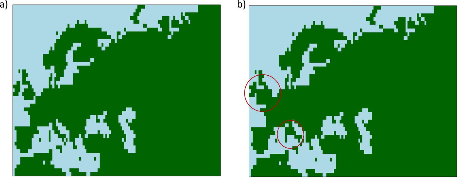
Maps showing areas where diffusion in the model is allowed (green) and where it is forbidden (blue).

(a) Map without land bridges. (b) Map containing land bridges indicated with red circles.

Appendix 2—figure 2

Download asset Open asset

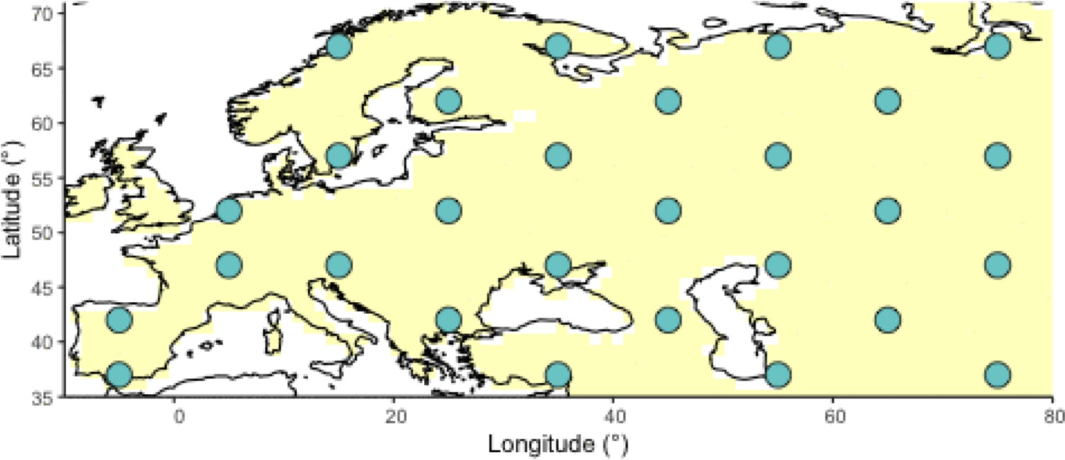
Geographic locations for points used as potential origins of the allele at the initialization of the simulated annealing optimization algorithm.

Note that, after initialization, the algorithm can continuously explore any points on the map grid that are not necessarily included in this point set.

Appendix 2—figure 3

Download asset Open asset

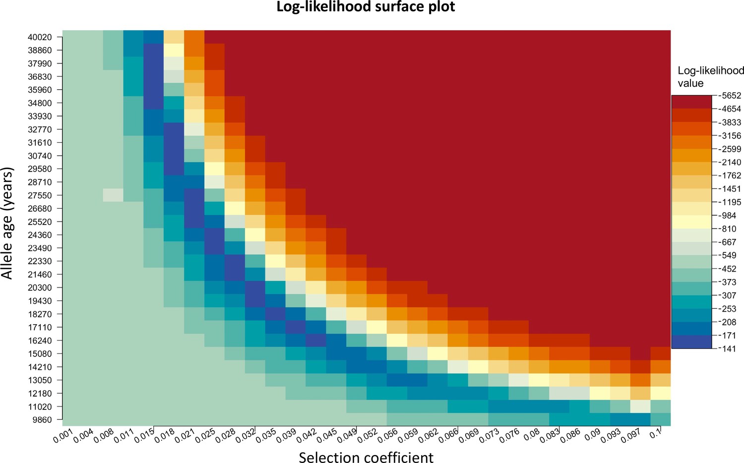
Log-likelihood as a function of selection coefficient and age of the allele.

Dark blue regions correspond to optimal solutions.

Appendix 2—table 1

Parameter values used to generate simulations using numerical solutions to Equation 3 compared to parameter estimates assuming model B.

The age of the allele was set to 29,000 years in all simulations. Columns named ‘long’ and ‘lat’ indicate the longitude and latitude of the geographic origin of the allele, respectively.

Simulation		$s$	$σ_{x}$ (km²/gen)	$σ_{y}$ (km²/gen)	Long	Lat
Simulation		True/pred (95% CI)	True/pred (95% CI)	True/pred (95% CI)	True/pred	True/pred
B1	Sample age >5000	0.02/0.0192 (0.0187 to 0.0196)	10/15.244 (2.5042 to 27.9828)	20/16.963 (11.9263 to 21.9993)	25/24	52/52
B1	Sample age <5000	0.02/0.0027 (0 to 0.0074)	10/8.805 (0.5631 to 17.0468)	20/97.432 (97.2566 to 97.6081)	–	–
B2	Sample age >5000	0.02/0.0193 (0.0189 to 0.0198)	10/15.348 (0 to 95.5192)	30/20.427 (0 to 51.514)	25/25	52/51
B2	Sample age <5000	0.02/0.001 (0 to 0.0059)	10/10.015 (1.6837 to 18.3472)	30/100 (99.9933 to 100.0067)	–	–
B3	Sample age >5000	0.02/0.0196 (0.0191 to 0.02)	10/8.149 (6.1551 to 10.143)	40/49.432 (0 to 135.9428)	25/24	52/51
B3	Sample age <5000	0.02/0.0265 (0.0145 to 0.0386)	10/7.855 (0 to 19.751)	40/100 (99.9933 to 100.0067)	–	–
B4	Sample age >5000	0.02/0.0188 (0.0188 to 0.0188)	20/19.037 (19.0311 to 19.0435)	10/19.254 (19.2439 to 19.2638)	25/25	52/51
B4	Sample age <5000	0.02/0.0142 (0.0111 to 0.0173)	20/17.354 (4.4083 to 30.2991)	10/1.489 (0 to 18.5993)	–	–
B5	Sample age >5000	0.02/0.0196 (0.019 to 0.0202)	30/26.409 (11.1997 to 41.6184)	10/11.429 (7.1825 to 15.6759)	25/27	52/51
B5	Sample age <5000	0.02/0.0215 (0.0183 to 0.0246)	30/14.3 (0 to 68.176)	10/1.554 (0 to 16.5985)	–	–
B6	Sample age >5000	0.02/0.0199 (0.0192 to 0.0206)	40/85.415 (41.6058 to 129.2248)	10/9.02 (7.2853 to 10.7538)	25/6	52/51
B6	Sample age <5000	0.02/0.0163 (0.0112 to 0.0213)	40/10.403 (0 to 22.533)	10/22.623 (12.0841 to 33.1614)	–	–

Appendix 2—table 2

Parameter values used to generate simulations using numerical solutions to Equation 4, compared to parameter estimates assuming model C.

The age of the allele was set to 29,000 years in all simulations. Columns named ‘long’ and ‘lat’ indicate the longitude and latitude of the geographic origin of the allele, respectively.

Simulation		$s$	$σ_{x}$ (km²/gen)	$σ_{y}$ (km²/gen)	v_x (km/gen)	v_y (km/gen)	Long	Lat
Simulation		True/pred (95% CI)	True/pred (95% CI)	True/pred (95% CI)	True/pred (95% CI)	True/pred (95% CI)	True/pred	True/pred
C1	Sample age >5000	0.02/0.0189 (0.0188 to 0.0189)	20/52.246 (52.2051 to 52.2872)	20/16.373 (16.332 to 16.4139)	-2/-1.675 (-1.6771 to -1.6722)	-2/-2.067 (-2.0702 to -2.0639)	25/4	52/45
C1	Sample age <5000	0.02/0.0231 (0.023 to 0.0233)	20/11.086 (10.9286 to 11.2441)	20/15.606 (15.3659 to 15.8467)	-2/0.399 (0.3946 to 0.4037)	-2/-2.491 (-2.5458 to -2.436)	–	–
C2	Sample age >5000	0.02/0.0185 (0.0176 to 0.0195)	10/19.434 (5.6736 to 33.1952)	20/18.727 (4.8938 to 32.5605)	-1.2/1.579 (1.2671 to 1.8905)	1.9/-0.801 (-1.1684 to -0.4331)	25/-6	52/38
C2	Sample age <5000	0.02/0.0205 (0.0175–0.0234)	10/38.144 (10.3123 to 65.9749)	20/51.094 (14.0489 to 88.1388)	-1.2/-1.299 (-2.7247 to 0.1266)	1.9/2.493 (2.4929 to 2.4933)	–	–
C3	Sample age >5000	0.02/0.0255 (0.0254–0.0256)	30/59.237 (59.1269 to 59.347)	10/6.604 (6.5991 to 6.6087)	1.8/2.195 (2.1918 to 2.1985)	-0.8/0.438 (0.4381 to 0.4387)	25/65	52/66
C3	Sample age <5000	0.02/0.0079 (0– 0.0165)	30/86.511 (0 to 194.0772)	10/40.693 (24.3946 to 56.9905)	1.8/-2.498 (-2.4983 to -2.498)	-0.8/-0.014 (-3.4481 to 3.4204)	–	–
C4	Sample age >5000	0.02/0.0197 (0.0191–0.0204)	10/19.647 (14.975 to 24.3197)	10/13.585 (0 to 27.2936)	1.2/-0.054 (-0.0968 to -0.0111)	1/0.72 (0.4278 to 1.0124)	25/44	52/50
C4	Sample age <5000	0.02/0.0137 (0.0046–0.0229)	10/14.151 (0 to 32.1031)	10/4.093 (0 to 49.4651)	1.2/0.8 (-3.4903 to 5.0895)	1/2.434 (2.4299 to 2.4387)	–	–

Appendix 2—table 3

Parameter value estimates for each of the nine clustering schemes and true parameter values used to generate the deterministic simulation.

The age of the allele was set to 17,400 years. Columns named ‘long’ and ‘lat’ indicate the longitude and latitude of the geographic origin of the allele, respectively.

Sampling scheme		$S$ (95% CI)	$σ_{x}$ (km2/gen) (95% CI)	$σ_{y}$ (km2/gen) (95% CI)	$v_{x}$ (km/gen) (95% CI)	$v_{y}$ (km/gen)(95% CI)	Long	Lat
Homogeneous 75%/25%	Sample age >5000	0.0385 (0.0364 to 0.0406)	24.592 (14.9174 to 34.2675)	16.194 (4.8309 to 27.5568)	-1.209 (-1.6947 to -0.7229)	-1.555 (-2.0804 to -1.0294)	44	48
Homogeneous 75%/25%	Sample age <5000	0.0261 (0.0201 to 0.0321)	45.725 (19.0071 to 72.4437)	11.95 (0.0000 to 27.2152)	2.499 (2.4993 to 2.4996)	-0.905 (-2.3876–0.5783)	44	48
Homogeneous 50%/50%	Sample age >5000	0.0379 (0.0364 to 0.0394)	23.071 (0.0000 to 66.2585)	11.455 (0.0000 to 26.4585)	-0.827 (-3.2669 to 1.6124)	-0.934 (-1.5199 to -0.3476)	46	51
Homogeneous 50%/50%	Sample age <5000	33.944 (0.0292 to 0.0385)	33.944 (13.1707 to 54.7167)	6.183 (0.0000 to 13.3805)	0.478 (-0.5529 to 1.5089)	0.315 (-0.1828–0.8127)	46	51
Homogeneous 25%/75%	Sample age >5000	0.0379 (0.0364 to 0.0394)	22.619 (14.8534 to 30.3839)	13.588 (6.1189 to 21.0574)	-1.4 (-1.9213 to -0.8782)	-1.021 (-1.4258 to -0.6161)	46	50
Homogeneous 25%/75%	Sample age <5000	0.0322 (0.0257 to 0.0388)	70.446 (24.6065 to 116.2854)	3.786 (0.0000 to 21.6379)	2.499 (2.4984 to 2.4987)	-0.99 (-2.0881 to 0.1079)	46	50
Intermediate 75%/25%	Sample age >5000	0.0378 (0.0378 to 0.0378)	20.905 (20.904 to 20.9065)	14.583 (14.5818 to 14.5844)	-1.069 (-1.0687 to -1.0684)	-0.547 (-0.5468 to -0.5467)	44	52
Intermediate 75%/25%	Sample age <5000	0.0342 (0.0276 to 0.0407)	70.405 (29.0665 to 111.7428)	1.936 (0.0000 to 18.9234)	2.5 (2.4995 to 2.4998)	-1.865 (-3.0637 to -0.6655)	44	52
Intermediate 50%/50%	Sample age >5000	0.0379 (0.0378–0.0379)	93.136 (93.0316 to 93.2406)	10.99 (10.9808 to 10.9994)	1.103 (1.1009 to 1.1048)	0.695 (0.6939–0.6954)	34	57
Intermediate 50%/50%	Sample age <5000	0.0327 (0.0288–0.0367)	22.409 (0.0000 to 69.8122)	18.11 (7.9198 to 28.2994)	2.496 (2.4962 to 2.4965)	-2.499 (-2.4992 to -2.4989)	34	57
Intermediate 25%/75%	Sample age >5000	0.0386 (0.0371–0.0402)	21.385 (14.0301 to 28.7407)	12.335 (3.3756 to 21.2943)	-1.028 (-1.4606 to -0.5956)	-1.307 (-1.7696 to -0.845)	43	49
Intermediate 25%/75%	Sample age <5000	0.0295 (0.026–0.0329)	21.197 (6.0797 to 36.3142)	11.318 (2.651 to 19.9851)	2.5 (2.4997 to 2.5000)	-0.757 (-1.391 to -0.123)	43	49
Extreme 75%/25%	Sample age >5000	0.0362 (0.0336–0.0389)	33.07 (0.0000 to 78.1418)	26.744 (0.0000 to 155.2413)	-0.087 (-0.3579 to 0.1832)	-2.001 (-4.7547–0.7524)	39	46
Extreme 75%/25%	Sample age <5000	0.0299 (0.0266–0.0332)	16.702 (0.0000 to 40.5995)	3.048 (0.0000 to 13.034)	2.197 (0.8463 to 3.5479)	-2.499 (-2.4995 to -2.4992)	39	46
Extreme 50%/50%	Sample age >5000	0.0392 (0.0369–0.0416)	95.472 (95.2997 to 95.6441)	11.22 (5.3235 to 17.1167)	1.633 (-2.5434 to 5.8102)	0.258 (0.0818–0.434)	36	57
Extreme 50%/50%	Sample age <5000	0.0355 (0.0314–0.0396)	11.756 (10.3763 to 13.1361)	11.817 (10.1474 to 13.4863)	2.5 (2.2069 to 2.7928)	-0.362 (-0.4325 to -0.2919)	36	57
Extreme 25%/75%	Sample age >5000	0.047 (0.047–0.047)	7.909 (7.9075 to 7.9106)	5.941 (5.9403 to 5.942)	0.454 (0.4537 to 0.4538)	-2.273 (-2.2732 to -2.2729)	34	38
Extreme 25%/75%	Sample age <5000	0.0434 (0.0385–0.0483)	40.097 (33.7903 to 46.4034)	12.118 (5.781 to 18.4555)	2.5 (1.6706 to 3.3285)	-1.435 (-2.3958 to -0.4736)	34	38
	True parameter values	0.04	25	10	1.8	-0.8	25	52

Appendix 2—table 4

Parameter values estimated using model C for the forward simulation created using SLiM.

Columns named ‘long’ and ‘lat’indicate the longitude and latitude of the geographic origin of the allele, respectively.

$s$ (95% CI)	$σ_{x}$ (km²/gen) (95% CI)	$σ_{y}$ (km²/gen)	v_x(km/gen)(95% CI)	v_y(km/gen)(95% CI)	Long	Lat	Allele age (years)
0.0366 (0.0357 to 0.0375)	58.583 (49.1983 to 67.9669)	63.733 (3.6601 to 123.8056)	-0.436 (-0.8077to -0.0649)	-1.564 (-3.0915 to -0.0355)	15	47	15,000

Appendix 2—table 5

Summary of parameter estimates for rs4988235(T).

The upper two rows correspond to results obtained assuming the allele age to be the point estimate of the start of selection onset from Itan et al., 2009: 7441 years ago. The middle two rows and the bottom two rows show results assuming the age to be either the lower or the higher ends of the age’s 95% confidence interval from Itan et al., 2009. Columns named ‘long’ and ‘Lat’ indicate the longitude and latitude of the geographic origin of the allele, respectively.

	$s$ (95% CI)	$σ_{x}$ (km²/gen) (95% CI)	$σ_{y}$ (km²/gen) (95% CI)	v_x (km/gen) (95% CI)	v_y (km/gen) (95% CI)	Long	Lat	Allele age (years)
Sample age >5000	0.0993 (0.0993 to 0.0993)	20.293 (15.5643 to 25.0226)	15.642 (9.9963 to 21.2871)	-0.575 (-0.8055 to -0.3446)	0.435 (0.319–0.5512)	43	51	7441
Sample age <5000	0.0328 (0.0327 to 0.0329)	94.901 (94.2585 to 95.5435)	85.612 (84.6975 to 86.526)	-1.211 (-1.2197 to -1.2019)	-2.5 (-2.5136 to -2.4855)	43	51	7441
Sample age >5000	0.0867 (0.0866 to 0.0867)	24.27 (24.2658 to 24.2734)	28.328 (28.3234 to 28.3326)	-0.398 (-0.3985 to -0.3984)	-2.055 (-2.0562 to -2.0547)	35	46	8683
Sample age <5000	0.0321 (0.0319–0.0323)	97.325 (97.1434–97.5061)	87.416 (85.6745 to 89.1578)	-2.5 (-2.5 to -2.4997)	-2.389 (-2.3935 to -2.3845)	35	46	8683
Sample age >5000	0.0994 (0.0994–0.0994)	22.92 (15.0004–30.8397)	17.884 (13.8709 to 21.8967)	0.327 (0.1726 to 0.4818)	-0.295 (-0.3678 to -0.2229)	35	49	6256
Sample age <5000	0.0572 (0.057–0.0574)	95.014 (93.6242–96.4032)	85.249 (82.9662 to 87.5322)	-2.499 (-2.4992 to -2.4989)	-1.679 (-1.7919 to -1.5658)	35	49	6256

Appendix 2—table 6

Parameter estimates for rs4988235(T) using the allele age inferred in Albers and McVean, 2020.

Columns named ‘long’ and ‘lat’ indicate the longitude and latitude of the geographic origin of the allele, respectively.

	$s$ (95% CI)	$σ_{x}$ (km²/gen) (95% CI)	$σ_{y}$ (km²/gen) (95% CI)	v_x (km/gen) (95% CI)	v_y (km/gen) (95% CI)	Long	Lat	Allele age (years)
Sample age >5000	0.0285 (0.0285 to 0.0285)	1.25 (1.2492 to 1.25)	44.619 (44.5944 to 44.6445)	-0.177 (-0.1773 to -0.1771)	1.925 (1.9247 to 1.9262)	32	66	20,106
Sample age <5000	0.0255 (0.0252 to 0.0258)	92.545 (91.6963 to 93.3941)	87.545 (85.3525 to 89.7369)	-2.499 (-2.4992 to -2.4989)	-2.271 (-2.4127 to -2.1297)	32	66	20,106

Appendix 2—table 7

Summary of parameter estimates for rs1042602(A).

Upper two rows correspond to model fit when allele age is set to be the point estimate Albers and McVean, 2020: 26,367 years ago. The middle two rows and the bottom two rows show results assuming the age to be either the lower or the higher ends of the allele age’s 95% confidence interval from Albers and McVean, 2020. Columns named ‘long’ and ‘lat’ indicate the longitude and latitude of the geographic origin of the allele, respectively.

	$s$ (95% CI)	σ_x(km²/gen) (95% CI)	σ_y (km²/gen) (95% CI)	v_x(km/gen) (95% CI)	v_y(km/gen) (95% CI)	Long	Lat	Allele age (years)
Sample age >5000	0.0221 (0.0216 to 0.0227)	71.668 (24.7274 to 118.6092)	50.434 (25.6535 to 75.2136)	-2.268 (-3.006 to -1.5304)	-0.486 (-0.8661 to -0.1053)	44	43	26,367
Sample age <5000	0.0102 (0.0083 to 0.012)	69.25 (14.0247 to 124.4756)	95.281 (95.1087 to 95.453)	0.849 (-0.0783 to 1.7769)	-0.503 (-0.929 to -0.076)	44	43	26,367
Sample age >5000	0.0214 (0.0205 to 0.0223)	57.914 (0 to 131.3177)	83.846 (0 to 246.6688)	-2.111 (-2.8784 to -1.3429)	1.305 (-0.8411 to 3.4519)	46	51	27,315
Sample age <5000	0.01 (0.0078 to 0.0121)	88.218 (0 to 190.105)	96.216 (96.0422 to 96.3898)	1.19 (-0.7489 to 3.1293)	-0.88 (-2.0897 to 0.3299)	46	51	27,315
Sample age >5000	0.023 (0.023 to 0.0231)	75.857 (75.8065 to 75.9071)	48.992 (48.9166 to 49.0674)	-2.362 (-2.3655 to -2.3593)	-0.837 (-0.8371 to -0.8362)	43	42	25,424
Sample age <5000	0.0099 (0.0085 to 0.0112)	72.847 (67.7991 to 77.8949)	92.867 (75.4925 to 110.2412)	0.497 (0.2717 to 0.7214)	-0.685 (-0.8076 to -0.5628)	43	42	25,424

Appendix 2—table 8

Summary of parameter estimates for rs4988235(T) when the origin of the allele is forced to be at different points in the map (top panel corresponds to the original fit for the geographic position).

In all cases, the estimated age of allele that was inputted into the model is 7441 years ago. Columns named ‘long’ and ‘lat’ indicate the longitude and latitude of the geographic origin of the allele, respectively.

	$s$ (95% CI)	$σ_{x}$ (km²/gen) (95% CI)	$σ_{y}$ (km²/gen) (95% CI)	v_x (km/gen) (95% CI)	v_y (km/gen) (95% CI)	Long	Lat
Sample age >5000	0.0993 (0.0993 to 0.0993)	20.293 (15.5643 to 25.0226)	15.642 (9.9963 to 21.2871)	-0.575 (-0.8055 to -0.3446)	0.435 (0.319 to 0.5512)	43	51
Sample age <5000	0.0328 (0.0327 to 0.0329)	94.901 (94.2585 to 95.5435)	85.612 (84.6975 to 86.526)	-1.211 (-1.2197 to -1.2019)	-2.5 (-2.5136 to -2.4855)	43	51
Sample age >5000	0.0985 (0.0985 to 0.0985)	3.103 (3.1027 to 3.1031)	44.876 (44.8747 to 44.8768)	0.354 (0.3537–0.3537)	-0.663 (-0.6634 to -0.6633)	33	51
Sample age <5000	0.0413 (0.0411 to 0.0415)	96.029 (95.8493 to 96.2087)	85.711 (83.6634 to 87.7594)	-2.5 (-2.5002 to -2.4998)	-1.318 (-1.46 to -1.1764)	33	51
Sample age >5000	0.0979 (0.0978 to 0.0979)	70.388 (70.3697 to 70.4065)	2.628 (2.6271 to 2.6286)	-2.328 (-2.3286 to -2.3276)	1.216 (1.2159–1.2164)	53	51
Sample age <5000	0.0376 (0.0374 to 0.0377)	3.705 (1.9497 to 5.4607)	77.019 (74.9065– to 79.1311)	-2.413 (-2.4174 to -2.4084)	-2.5 (-2.4999 to -2.4995)	53	51
Sample age >5000	0.0991 (0.0991 to 0.0992)	1.218 (1.218 to 1.2183)	15.127 (15.1256 to 15.1287)	-0.781 (-0.781 to -0.7807)	2.452 (2.452 to 2.4526)	43	61
Sample age <5000	0.0359 (0.0357 to 0.0361)	96.836 (96.6538 to 97.0183)	86.616 (83.9434 to 89.2891)	-2.499 (-2.4994 to -2.499)	-2.219 (-2.3368 to -2.1009)	43	61
Sample age >5000	0.0999 (0.0999 to 0.0999)	27.442 (27.4385 to 27.4464)	11.879 (11.8781 to 11.8801)	-1.582 (-1.5824 to -1.582)	-1.638 (-1.6382 to -1.638)	43	41
Sample age <5000	0.0355 (0.0353 to 0.0357)	97.044 (96.8637 to 97.2236)	86.223 (83.4533 to 88.992)	-2.499 (-2.4996 to -2.4992)	-2.148 (-2.2811 to -2.0141)	43	41

Appendix 2—table 9

Parameter estimates for rs4988235(T) using the geographic origin of the allele inferred in Itan et al., 2009.

Columns named ‘long’ and ‘lat’ indicate the longitude and latitude of the geographic origin of the allele, respectively.

	$s$ (95% CI)	$σ_{x}$ (km²/gen) (95% CI)	$σ_{y}$ (km²/gen) (95% CI)	v_x (km/gen) (95% CI)	v_y (km/gen) (95% CI)	Long	Lat	Allele age (years)
Sample age >5000	0.0989 (0.0989 to 0.0989)	9.341 (9.3402 to 9.341)	3.264 (3.2635 to 3.2643)	2.338 (2.3379 to 2.3381)	-0.21 (-0.2098 to -0.2098)	13	48	7441
Sample age <5000	0.0358 (0.0357 to 0.036)	97.086 (96.9059 to 97.2657)	87.043 (85.1968 to 88.8895)	-2.434 (-2.4385 to -2.4294)	-2.499 (-2.4994 to -2.499)	13	48	7441

Appendix 2—table 10

Summary of parameter estimates for rs1042602(A) when the origin of the allele is forced to be at different points in the map (top panel corresponds to the original fit for the geographic position).

In all cases, the estimated age of allele that was inputted into the model is 26,367 years ago. Columns named ‘long’ and ‘lat’ indicate the longitude and latitude of the geographic origin of the allele, respectively.

	$s$ (95% CI)	$σ_{x}$ (km²/gen) (95% CI)	$σ_{y}$ (km²/gen) (95% CI)	v_x (km/gen) (95% CI)	v_y (km/gen) (95% CI)	Long	Lat
Sample age >5000	0.0221 (0.0216 to 0.0227)	71.668 (24.7274 to 118.6092)	50.434 (25.6535 to 75.2136)	-2.268 (-3.006 to -1.5304)	-0.486 (-0.8661 to -0.1053)	44	43
Sample age <5000	0.0102 (0.0083 to 0.012)	69.25 (14.0247 to 124.4756)	95.281 (95.1087 to 95.453)	0.849 (-0.0783 to 1.7769)	-0.503 (-0.929 to -0.076)	44	43
Sample age >5000	0.0227 (0.0223 to 0.0231)	42.745 (33.6354 to 51.8541)	96.993 (96.8183 to 97.1683)	-2.437 (-2.4412 to -2.4324)	-0.266 (-0.4848 to -0.0468)	54	43
Sample age <5000	0.0095 (0.007 to 0.0119)	93.477 (7.6582 to 179.2965)	99.634 (0 to 205.4586)	-2.499 (-3.2101 to -1.7873)	2.057 (-0.7888 to 4.903)	54	43
Sample age >5000	0.0221 (0.0221 to 0.0221)	47.691 (47.6686 to 47.7127)	71.367 (71.336 to 71.3986)	-2.164 (-2.1652 to -2.1637)	1.839 (1.8387 to 1.8392)	44	53
Sample age <5000	0.0112 (0.0093 to 0.0131)	87.959 (0 to 215.8939)	88.951 (25.5422 to 152.3589)	2.108 (-0.2061 to 4.4227)	-2.237 (-5.7828 to 1.3083)	44	53
Sample age >5000	0.0219 (0.0209 to 0.0229)	73.106 (38.1699 to 108.043)	76.835 (24.0025 to 129.6684)	-2.429 (-2.4335 to -2.4248)	-1.474 (-2.8769 to -0.0706)	44	33
Sample age <5000	0.0102(0.0083 to 0.0121)	88.216 (0 to 192.1057)	95.401 (95.2283 to 95.573)	0.871 (-0.2474 to 1.9893)	-1.026 (-2.6161 to 0.564)	44	33

Data availability

The current manuscript is a computational study, therefore no data have been generated for this manuscript. Software code along with publicly available data used for this study are deposited to GitHub: https://github.com/RasaMukti/stepadna/tree/main/reproducibles (copy archived at swh:1:rev:d024767648d873f329a8e17fcaf6034c99157120).

The following previously published data sets were used

1. Reich D
2. Mallick S
(2019) Allen Ancient DNA
ID AADR. Allen Ancient DNA Resource (AADR).

https://reich.hms.harvard.edu/allen-ancient-dna-resource-aadr-downloadable-genotypes-present-day-and-ancient-dna-data
1. Bergström A
2. McCarthy SA
3. Hui R
4. Almarri MA
5. Ayub Q
6. Danecek P
7. Chen Y
8. Felkel S
9. Hallast P
10. Kamm J
11. Blanché H
12. Deleuze JF
13. Cann H
14. Mallick S
15. Reich D
16. Sandhu MS
17. Skoglund P
18. Scally A
19. Xue Y
20. Durbin R
21. Tyler-Smith C
(2020) EMBL-EBI
ID HGDP. Human Genome Diversity Panel.

http://ftp.1000genomes.ebi.ac.uk/vol1/ftp/data_collections/HGDP/

References

1. Albers PK
2. McVean G
(2020) Dating genomic variants and shared ancestry in population-scale sequencing data
PLOS Biology 18:e3000586.
https://doi.org/10.1371/journal.pbio.3000586
- PubMed
- Google Scholar
1. Allentoft ME
2. Sikora M
3. Sjögren K-G
4. Rasmussen S
5. Rasmussen M
6. Stenderup J
7. Damgaard PB
8. Schroeder H
9. Ahlström T
10. Vinner L
11. Malaspinas A-S
12. Margaryan A
13. Higham T
14. Chivall D
15. Lynnerup N
16. Harvig L
17. Baron J
18. Della Casa P
19. Dąbrowski P
20. Duffy PR
21. Ebel AV
22. Epimakhov A
23. Frei K
24. Furmanek M
25. Gralak T
26. Gromov A
27. Gronkiewicz S
28. Grupe G
29. Hajdu T
30. Jarysz R
31. Khartanovich V
32. Khokhlov A
33. Kiss V
34. Kolář J
35. Kriiska A
36. Lasak I
37. Longhi C
38. McGlynn G
39. Merkevicius A
40. Merkyte I
41. Metspalu M
42. Mkrtchyan R
43. Moiseyev V
44. Paja L
45. Pálfi G
46. Pokutta D
47. Pospieszny Ł
48. Price TD
49. Saag L
50. Sablin M
51. Shishlina N
52. Smrčka V
53. Soenov VI
54. Szeverényi V
55. Tóth G
56. Trifanova SV
57. Varul L
58. Vicze M
59. Yepiskoposyan L
60. Zhitenev V
61. Orlando L
62. Sicheritz-Pontén T
63. Brunak S
64. Nielsen R
65. Kristiansen K
66. Willerslev E
(2015) Population genomics of bronze age Eurasia
Nature 522:167–172.
https://doi.org/10.1038/nature14507
- PubMed
- Google Scholar
(2008) Complex signatures of selection for the melanogenic loci Tyr, TYRP1 and DCT in humans
BMC Evolutionary Biology 8:1–14.
https://doi.org/10.1186/1471-2148-8-74
- PubMed
- Google Scholar
1. Bélisle CJP
(1992) Convergence theorems for a class of simulated annealing algorithms on rd
Journal of Applied Probability 29:885–895.
https://doi.org/10.2307/3214721
- Google Scholar
1. Bergström A
2. McCarthy SA
3. Hui R
4. Almarri MA
5. Ayub Q
6. Danecek P
7. Chen Y
8. Felkel S
9. Hallast P
10. Kamm J
11. Blanché H
12. Deleuze J-F
13. Cann H
14. Mallick S
15. Reich D
16. Sandhu MS
17. Skoglund P
18. Scally A
19. Xue Y
20. Durbin R
21. Tyler-Smith C
(2020) Insights into human genetic variation and population history from 929 diverse genomes
Science 367:eaay5012.
https://doi.org/10.1126/science.aay5012
- PubMed
- Google Scholar
(2004) Genetic signatures of strong recent positive selection at the lactase gene
American Journal of Human Genetics 74:1111–1120.
https://doi.org/10.1086/421051
- PubMed
- Google Scholar
Software
1. Bolker B
(2020) Bbmle: tools for general maximum likelihood estimation, version 1.0.23.1
R Package.

https://CRAN.R-project.org/package=bbmle
(2016) A spatial framework for understanding population structure and admixture
PLOS Genetics 12:e1005703.
https://doi.org/10.1371/journal.pgen.1005703
- PubMed
- Google Scholar
1. Bradburd GS
2. Ralph PL
(2019) Spatial population genetics: it’s about time
Annual Review of Ecology, Evolution, and Systematics 50:427–449.
https://doi.org/10.1146/annurev-ecolsys-110316-022659
- Google Scholar
(2000) Blur-generated non-separable space-time models
Journal of the Royal Statistical Society 62:847–860.
https://doi.org/10.1111/1467-9868.00269
- Google Scholar
1. Burger J
2. Kirchner M
3. Bramanti B
4. Haak W
5. Thomas MG
(2007) Absence of the lactase-persistence-associated allele in early neolithic europeans
PNAS 104:3736–3741.
https://doi.org/10.1073/pnas.0607187104
- PubMed
- Google Scholar
1. Burger J
2. Link V
3. Blöcher J
4. Schulz A
5. Sell C
6. Pochon Z
7. Diekmann Y
8. Žegarac A
9. Hofmanová Z
10. Winkelbach L
11. Reyna-Blanco CS
12. Bieker V
13. Orschiedt J
14. Brinker U
15. Scheu A
16. Leuenberger C
17. Bertino TS
18. Bollongino R
19. Lidke G
20. Stefanović S
21. Jantzen D
22. Kaiser E
23. Terberger T
24. Thomas MG
25. Veeramah KR
26. Wegmann D
(2020) Low prevalence of lactase persistence in bronze age europe indicates ongoing strong selection over the last 3,000 years
Current Biology 30:4307–4315.
https://doi.org/10.1016/j.cub.2020.08.033
- PubMed
- Google Scholar
1. Byrd RH
2. Lu P
3. Nocedal J
4. Zhu C
(1995) A limited memory algorithm for bound constrained optimization
SIAM Journal on Scientific Computing 16:1190–1208.
https://doi.org/10.1137/0916069
- Google Scholar
Book
1. Cantrell RS
2. Cosner C
(2004) Spatial Ecology via Reaction‐Diffusion Equations
John Wiley & Sons.
https://doi.org/10.1002/0470871296
- Google Scholar
Book
1. Casella G
2. Berger RL
(2001)
Statistical Inference (Second)

Belmont, USA: Cengage Learning.
- Google Scholar
(2019) The evolutionary genetics of lactase persistence in seven ethnic groups across the iranian plateau
Human Genomics 13:7.
https://doi.org/10.1186/s40246-019-0195-5
- PubMed
- Google Scholar
Book
1. Colin McEvedy RJ
(1978)
Atlas of World Population History

Great Britain: Penguin Books Lyd. and Allen Lane.
- Google Scholar
Book
1. Cressie N
2. Wikle CK
(2015) Statistics for Spatio-Temporal Data
Hoboken, New Jersey, USA: John Wiley & Sons.
https://doi.org/10.1111/j.1538-4632.2012.00859.x
- Google Scholar
Book
1. Crow JF
2. Kimura M
(1970)
An Introduction to Population Genetics Theory

Burgess Publishing Company.
- Google Scholar
(2020) Inference of natural selection from ancient DNA
Evolution Letters 4:94–108.
https://doi.org/10.1002/evl3.165
- PubMed
- Google Scholar
Book
1. Efron B
2. Hastie T
(2016) Computer Age Statistical Inference
Cambridge University Press.
https://doi.org/10.1017/CBO9781316576533
- Google Scholar
(2002) Identification of a variant associated with adult-type hypolactasia
Nature Genetics 30:233–237.
https://doi.org/10.1038/ng826
- PubMed
- Google Scholar
1. Enattah NS
2. Jensen TGK
3. Nielsen M
4. Lewinski R
5. Kuokkanen M
6. Rasinpera H
7. El-Shanti H
8. Seo JK
9. Alifrangis M
10. Khalil IF
11. Natah A
12. Ali A
13. Natah S
14. Comas D
15. Mehdi SQ
16. Groop L
17. Vestergaard EM
18. Imtiaz F
19. Rashed MS
20. Meyer B
21. Troelsen J
22. Peltonen L
(2008) Independent introduction of two lactase-persistence alleles into human populations reflects different history of adaptation to milk culture
American Journal of Human Genetics 82:57–72.
https://doi.org/10.1016/j.ajhg.2007.09.012
- PubMed
- Google Scholar
Book
1. Ewens WJ
(2012) Mathematical Population Genetics 1: Theoretical Introduction
Springer Science & Business Media.
https://doi.org/10.1007/978-0-387-21822-9
- Google Scholar
1. Fisher RA
(1922) On the mathematical foundations of theoretical statistics
Philosophical Transactions of the Royal Society of London. Series A, Containing Papers of A Mathematical or Physical Character 222:309–368.
https://doi.org/10.1098/rsta.1922.0009
- Google Scholar
1. Fisher RA
(1937) The wave of advance of advantageous genes
Annals of Eugenics 7:355–369.
https://doi.org/10.1111/j.1469-1809.1937.tb02153.x
- Google Scholar
1. Gallego Romero I
2. Basu Mallick C
3. Liebert A
4. Crivellaro F
5. Chaubey G
6. Itan Y
7. Metspalu M
8. Eaaswarkhanth M
9. Pitchappan R
10. Villems R
11. Reich D
12. Singh L
13. Thangaraj K
14. Thomas MG
15. Swallow DM
16. Mirazón Lahr M
17. Kivisild T
(2012) Herders of Indian and European cattle share their predominant allele for lactase persistence
Molecular Biology and Evolution 29:249–260.
https://doi.org/10.1093/molbev/msr190
- PubMed
- Google Scholar
1. Gamba C
2. Jones ER
3. Teasdale MD
4. McLaughlin RL
5. Gonzalez-Fortes G
6. Mattiangeli V
7. Domboróczki L
8. Kővári I
9. Pap I
10. Anders A
11. Whittle A
12. Dani J
13. Raczky P
14. Higham TFG
15. Hofreiter M
16. Bradley DG
17. Pinhasi R
(2014) Genome flux and stasis in a five millennium transect of European prehistory
Nature Communications 5:1–9.
https://doi.org/10.1038/ncomms6257
- PubMed
- Google Scholar
(2009) Impact of selection and demography on the diffusion of lactase persistence
PLOS ONE 4:e6369.
https://doi.org/10.1371/journal.pone.0006369
- PubMed
- Google Scholar
1. Günther T
2. Malmström H
3. Svensson EM
4. Omrak A
5. Sánchez-Quinto F
6. Kılınç GM
7. Krzewińska M
8. Eriksson G
9. Fraser M
10. Edlund H
11. Munters AR
12. Coutinho A
13. Simões LG
14. Vicente M
15. Sjölander A
16. Jansen Sellevold B
17. Jørgensen R
18. Claes P
19. Shriver MD
20. Valdiosera C
21. Netea MG
22. Apel J
23. Lidén K
24. Skar B
25. Storå J
26. Götherström A
27. Jakobsson M
(2018) Population genomics of mesolithic Scandinavia: investigating early postglacial migration routes and high-latitude adaptation
PLOS Biology 16:e2003703.
https://doi.org/10.1371/journal.pbio.2003703
- PubMed
- Google Scholar
1. Haak W
2. Lazaridis I
3. Patterson N
4. Rohland N
5. Mallick S
6. Llamas B
7. Brandt G
8. Nordenfelt S
9. Harney E
10. Stewardson K
11. Fu Q
12. Mittnik A
13. Bánffy E
14. Economou C
15. Francken M
16. Friederich S
17. Pena RG
18. Hallgren F
19. Khartanovich V
20. Khokhlov A
21. Kunst M
22. Kuznetsov P
23. Meller H
24. Mochalov O
25. Moiseyev V
26. Nicklisch N
27. Pichler SL
28. Risch R
29. Rojo Guerra MA
30. Roth C
31. Szécsényi-Nagy A
32. Wahl J
33. Meyer M
34. Krause J
35. Brown D
36. Anthony D
37. Cooper A
38. Alt KW
39. Reich D
(2015) Massive migration from the steppe was a source for Indo-European languages in Europe
Nature 522:207–211.
https://doi.org/10.1038/nature14317
- PubMed
- Google Scholar
1. Hallatschek O
2. Fisher DS
(2014) Acceleration of evolutionary spread by long-range dispersal
PNAS 111:E4911–E4919.
https://doi.org/10.1073/pnas.1404663111
- PubMed
- Google Scholar
1. Haller BC
2. Messer PW
(2019) Slim 3: forward genetic simulations beyond the Wright-Fisher model
Molecular Biology and Evolution 36:632–637.
https://doi.org/10.1093/molbev/msy228
- PubMed
- Google Scholar
1. Hermisson J.
2. Pennings PS
(2005) Soft sweeps: molecular population genetics of adaptation from standing genetic variation
Genetics 169:2335–2352.
https://doi.org/10.1534/genetics.104.036947
- PubMed
- Google Scholar
(2017) Soft sweeps and beyond: understanding the patterns and probabilities of selection footprints under rapid adaptation
Methods in Ecology and Evolution 8:700–716.
https://doi.org/10.1111/2041-210X.12808
- Google Scholar
1. Heyer E
2. Brazier L
3. Ségurel L
4. Hegay T
5. Austerlitz F
6. Quintana-Murci L
7. Georges M
8. Pasquet P
9. Veuille M
(2011) Lactase persistence in central Asia: phenotype, genotype, and evolution
Human Biology 83:379–392.
https://doi.org/10.3378/027.083.0304
- PubMed
- Google Scholar
1. Hindmarsh AC
(1983) ODEPACK, A systematized collection of ODE solvers
Scientific Computing 1:55–64.
https://doi.org/10.12691/ajmo-4-1-1
- Google Scholar
(2013) Global patterns of diversity and selection in human tyrosinase gene
PLOS ONE 8:e74307.
https://doi.org/10.1371/journal.pone.0074307
- PubMed
- Google Scholar
(2021) Quantitative human paleogenetics: what can ancient DNA tell us about complex trait evolution?
Frontiers in Genetics 12:703541.
https://doi.org/10.3389/fgene.2021.703541
- PubMed
- Google Scholar
1. Itan Y
2. Powell A
3. Beaumont MA
4. Burger J
5. Thomas MG
(2009) The origins of lactase persistence in europe
PLOS Computational Biology 5:e1000491.
https://doi.org/10.1371/journal.pcbi.1000491
- Google Scholar
1. Itan Y
2. Jones BL
3. Ingram CJE
4. Swallow DM
5. Thomas MG
(2010) A worldwide correlation of lactase persistence phenotype and genotypes
BMC Evolutionary Biology 10:36.
https://doi.org/10.1186/1471-2148-10-36
- PubMed
- Google Scholar
1. Ju D
2. Mathieson I
(2020) The evolution of skin pigmentation associated variation in West Eurasia
PNAS 118:e2009227118.
https://doi.org/10.1073/pnas.2009227118
- Google Scholar
Book
1. Karlin S
2. Taylor H
(1975) A First Course in Stochastic Processes (Second)
New York: Academic Press.
https://doi.org/10.1016/C2009-1-28569-8
- Google Scholar
(2006) The fate of mutations surfing on the wave of a range expansion
Molecular Biology and Evolution 23:482–490.
https://doi.org/10.1093/molbev/msj057
- PubMed
- Google Scholar
(1937) A study of the diffusion equation with increase in the amount of substance, and its application to A biological problem
Byull 1:1–26.
https://doi.org/10.1007/978-94-011-3030-1_38
- Google Scholar
(2014) ANGSD: analysis of next generation sequencing data
BMC Bioinformatics 15:356.
https://doi.org/10.1186/s12859-014-0356-4
- PubMed
- Google Scholar
1. Krüttli A
2. Bouwman A
3. Akgül G
4. Della Casa P
5. Rühli F
6. Warinner C
7. Gilbert T
(2014) Ancient DNA analysis reveals high frequency of European lactase persistence allele (t-13910) in medieval central Europe
PLOS ONE 9:e86251.
https://doi.org/10.1371/journal.pone.0086251
- Google Scholar
(2007) Signatures of positive selection in genes associated with human skin pigmentation as revealed from analyses of single nucleotide polymorphisms
Annals of Human Genetics 71:354–369.
https://doi.org/10.1111/j.1469-1809.2006.00341.x
- PubMed
- Google Scholar
1. Li H
(2011) A statistical framework for SNP calling, mutation discovery, association mapping and population genetical parameter estimation from sequencing data
Bioinformatics 27:2987–2993.
https://doi.org/10.1093/bioinformatics/btr509
- PubMed
- Google Scholar
1. Liebert A
2. López S
3. Jones BL
4. Montalva N
5. Gerbault P
6. Lau W
7. Thomas MG
8. Bradman N
9. Maniatis N
10. Swallow DM
(2017) World-Wide distributions of lactase persistence alleles and the complex effects of recombination and selection
Human Genetics 136:1445–1453.
https://doi.org/10.1007/s00439-017-1847-y
- PubMed
- Google Scholar
(2017) Estimating mobility using sparse data: application to human genetic variation
PNAS 114:12213–12218.
https://doi.org/10.1073/pnas.1703642114
- PubMed
- Google Scholar
(2012) Estimating allele age and selection coefficient from time-serial data
Genetics 192:599–607.
https://doi.org/10.1534/genetics.112.140939
- PubMed
- Google Scholar
1. Marchi N
2. Mennecier P
3. Georges M
4. Lafosse S
5. Hegay T
6. Dorzhu C
7. Chichlo B
8. Ségurel L
9. Heyer E
(2018) Close inbreeding and low genetic diversity in inner Asian human populations despite geographical exogamy
Scientific Reports 8:9397.
https://doi.org/10.1038/s41598-018-27047-3
- PubMed
- Google Scholar
1. Marciniak S
2. Perry GH
(2017) Harnessing ancient genomes to study the history of human adaptation
Nature Reviews. Genetics 18:659–674.
https://doi.org/10.1038/nrg.2017.65
- PubMed
- Google Scholar
1. Margaryan A
2. Lawson DJ
3. Sikora M
4. Racimo F
5. Rasmussen S
6. Moltke I
7. Cassidy LM
8. Jørsboe E
9. Ingason A
10. Pedersen MW
11. Korneliussen T
12. Wilhelmson H
13. Buś MM
14. de Barros Damgaard P
15. Martiniano R
16. Renaud G
17. Bhérer C
18. Moreno-Mayar JV
19. Fotakis AK
20. Allen M
21. Allmäe R
22. Molak M
23. Cappellini E
24. Scorrano G
25. McColl H
26. Buzhilova A
27. Fox A
28. Albrechtsen A
29. Schütz B
30. Skar B
31. Arcini C
32. Falys C
33. Jonson CH
34. Błaszczyk D
35. Pezhemsky D
36. Turner-Walker G
37. Gestsdóttir H
38. Lundstrøm I
39. Gustin I
40. Mainland I
41. Potekhina I
42. Muntoni IM
43. Cheng J
44. Stenderup J
45. Ma J
46. Gibson J
47. Peets J
48. Gustafsson J
49. Iversen KH
50. Simpson L
51. Strand L
52. Loe L
53. Sikora M
54. Florek M
55. Vretemark M
56. Redknap M
57. Bajka M
58. Pushkina T
59. Søvsø M
60. Grigoreva N
61. Christensen T
62. Kastholm O
63. Uldum O
64. Favia P
65. Holck P
66. Sten S
67. Arge SV
68. Ellingvåg S
69. Moiseyev V
70. Bogdanowicz W
71. Magnusson Y
72. Orlando L
73. Pentz P
74. Jessen MD
75. Pedersen A
76. Collard M
77. Bradley DG
78. Jørkov ML
79. Arneborg J
80. Lynnerup N
81. Price N
82. Gilbert MTP
83. Allentoft ME
84. Bill J
85. Sindbæk SM
86. Hedeager L
87. Kristiansen K
88. Nielsen R
89. Werge T
90. Willerslev E
(2020) Population genomics of the Viking world
Nature 585:390–396.
https://doi.org/10.1038/s41586-020-2688-8
- PubMed
- Google Scholar
1. Mathieson I.
2. McVean G
(2014) Demography and the age of rare variants
PLOS Genetics 10:e1004528.
https://doi.org/10.1371/journal.pgen.1004528
- PubMed
- Google Scholar
1. Mathieson Iain
2. Lazaridis I
3. Rohland N
4. Mallick S
5. Patterson N
6. Roodenberg SA
7. Harney E
8. Stewardson K
9. Fernandes D
10. Novak M
11. Sirak K
12. Gamba C
13. Jones ER
14. Llamas B
15. Dryomov S
16. Pickrell J
17. Arsuaga JL
18. de Castro JMB
19. Carbonell E
20. Gerritsen F
21. Khokhlov A
22. Kuznetsov P
23. Lozano M
24. Meller H
25. Mochalov O
26. Moiseyev V
27. Guerra MAR
28. Roodenberg J
29. Vergès JM
30. Krause J
31. Cooper A
32. Alt KW
33. Brown D
34. Anthony D
35. Lalueza-Fox C
36. Haak W
37. Pinhasi R
38. Reich D
(2015) Genome-Wide patterns of selection in 230 ancient Eurasians
Nature 528:499–503.
https://doi.org/10.1038/nature16152
- PubMed
- Google Scholar
1. Mathieson S
2. Mathieson I
(2018) Fads1 and the timing of human adaptation to agriculture
Molecular Biology and Evolution 35:2957–2970.
https://doi.org/10.1093/molbev/msy180
- PubMed
- Google Scholar
Preprint
1. Mathieson I
(2020) Estimating Time-Varying Selection Coefficients from Time Series Data of Allele Frequencies
bioRxiv.
https://doi.org/10.1101/2020.11.17.387761
- Google Scholar
Software
1. Muktupavela R
(2021) Stepadna, version swh:1:rev:d024767648d873f329a8e17fcaf6034c99157120
Software Heritage.

https://archive.softwareheritage.org/swh:1:dir:8f71fa11f0316162937e47e32f43ceddad8f8332;origin=https://github.com/RasaMukti/stepadna;visit=swh:1:snp:d9b4d676338244c557777ef5c2a70ff0df2b68c0;anchor=swh:1:rev:d024767648d873f329a8e17fcaf6034c99157120
(2019) Inferring the model and onset of natural selection under varying population size from the site frequency spectrum and haplotype structure
Proceedings. Biological Sciences 286:20182541.
https://doi.org/10.1098/rspb.2018.2541
- PubMed
- Google Scholar
Book
1. NOAA, National Geophysical Data Center, B. C
(1988)
Data Announcement 88-MGG-02,, Digital Relief of the Surface of the Earth

Publisher: U.S. Department of Commerce.
- Google Scholar
(2005) The geographic spread of the CCR5 delta32 HIV-resistance allele
PLOS Biology 3:11.
https://doi.org/10.1371/journal.pbio.0030339
- PubMed
- Google Scholar
1. Novembre J
2. Han E
(2012) Human population structure and the adaptive response to pathogen-induced selection pressures
Philosophical Transactions of the Royal Society of London. Series B, Biological Sciences 367:878–886.
https://doi.org/10.1098/rstb.2011.0305
- PubMed
- Google Scholar
Book
1. Okubo A
(1980) Diffusion and ecological problems: mathematical models
In: Andersson S, editors. Biomathematics. Berlin, Heidelberg & New York: Springer-Verlag. pp. 254–272.
https://doi.org/10.1016/B978-0-444-50273-5.X5025-3
- Google Scholar
(1988) Models of dispersal in biological systems
Journal of Mathematical Biology 26:263–298.
https://doi.org/10.1007/BF00277392
- PubMed
- Google Scholar
1. Painter KJ
2. Hillen T
(2018) From random walks to fully anisotropic diffusion models for cell and animal movement
In Cell Movement 786:103–141.
https://doi.org/10.1007/978-3-319-96842-1_5
- Google Scholar
(2012) Distinguishing between selective sweeps from standing variation and from a de novo mutation
PLOS Genetics 8:e1003011.
https://doi.org/10.1371/journal.pgen.1003011
- PubMed
- Google Scholar
Software
1. Petr M
(2021) Bodkan/slendr, version 0.4.0
Github.

https://github.com/bodkan/slendr/
1. Pickrell JK
2. Coop G
3. Novembre J
4. Kudaravalli S
5. Li JZ
6. Absher D
7. Srinivasan BS
8. Barsh GS
9. Myers RM
10. Feldman MW
11. Pritchard JK
(2009) Signals of recent positive selection in a worldwide sample of human populations
Genome Research 19:826–837.
https://doi.org/10.1101/gr.087577.108
- PubMed
- Google Scholar
1. Platt A
2. Pivirotto A
3. Knoblauch J
4. Hey J
(2019) An estimator of first coalescent time reveals selection on young variants and large heterogeneity in rare allele ages among human populations
PLOS Genetics 15:e1008340.
https://doi.org/10.1371/journal.pgen.1008340
- PubMed
- Google Scholar
1. Pritchard JK
2. Di Rienzo A
(2010) Adaptation-not by sweeps alone
Nature Reviews. Genetics 11:665–667.
https://doi.org/10.1038/nrg2880
- PubMed
- Google Scholar
(2020a) Beyond broad strokes: sociocultural insights from the study of ancient genomes
Nature Reviews. Genetics 21:355–366.
https://doi.org/10.1038/s41576-020-0218-z
- PubMed
- Google Scholar
(2020b) The spatiotemporal spread of human migrations during the european holocene
PNAS 117:8989–9000.
https://doi.org/10.1073/pnas.1920051117
- PubMed
- Google Scholar
1. Ralph P
2. Coop G
(2010) Parallel adaptation: one or many waves of advance of an advantageous allele?
Genetics 186:647–668.
https://doi.org/10.1534/genetics.110.119594
- PubMed
- Google Scholar
1. Ray N
2. Excoffier L
(2009) Inferring past demography using spatially explicit population genetic models
Human Biology 81:141–157.
https://doi.org/10.3378/027.081.0303
- PubMed
- Google Scholar
Software
1. Reich D
2. Mallick S
(2019) Allen ancient dna resource (aadr): downloadable genotypes of present-day and ancient dna data, version V54.1
AADR.

https://reich.hms.harvard.edu/allen-ancient-dna-resource-aadr-downloadable-genotypes-present-day-and-ancient-dna-data
1. Sabeti PC
2. Walsh E
3. Schaffner SF
4. Varilly P
5. Fry B
6. Hutcheson HB
7. Cullen M
8. Mikkelsen TS
9. Roy J
10. Patterson N
11. Cooper R
12. Reich D
13. Altshuler D
14. O’Brien S
15. Lander ES
(2005) The case for selection at CCR5-delta32
PLOS Biology 3:e378.
https://doi.org/10.1371/journal.pbio.0030378
- PubMed
- Google Scholar
1. Sabeti PC
2. Varilly P
3. Fry B
4. Lohmueller J
5. Hostetter E
6. Cotsapas C
7. Xie X
8. Byrne EH
9. McCarroll SA
10. Gaudet R
11. Schaffner SF
12. Lander ES
13. International HapMap Consortium
14. Frazer KA
15. Ballinger DG
16. Cox DR
17. Hinds DA
18. Stuve LL
19. Gibbs RA
20. Belmont JW
21. Boudreau A
22. Hardenbol P
23. Leal SM
24. Pasternak S
25. Wheeler DA
26. Willis TD
27. Yu F
28. Yang H
29. Zeng C
30. Gao Y
31. Hu H
32. Hu W
33. Li C
34. Lin W
35. Liu S
36. Pan H
37. Tang X
38. Wang J
39. Wang W
40. Yu J
41. Zhang B
42. Zhang Q
43. Zhao H
44. Zhao H
45. Zhou J
46. Gabriel SB
47. Barry R
48. Blumenstiel B
49. Camargo A
50. Defelice M
51. Faggart M
52. Goyette M
53. Gupta S
54. Moore J
55. Nguyen H
56. Onofrio RC
57. Parkin M
58. Roy J
59. Stahl E
60. Winchester E
61. Ziaugra L
62. Altshuler D
63. Shen Y
64. Yao Z
65. Huang W
66. Chu X
67. He Y
68. Jin L
69. Liu Y
70. Shen Y
71. Sun W
72. Wang H
73. Wang Y
74. Wang Y
75. Xiong X
76. Xu L
77. Waye MMY
78. Tsui SKW
79. Xue H
80. Wong JT-F
81. Galver LM
82. Fan J-B
83. Gunderson K
84. Murray SS
85. Oliphant AR
86. Chee MS
87. Montpetit A
88. Chagnon F
89. Ferretti V
90. Leboeuf M
91. Olivier J-F
92. Phillips MS
93. Roumy S
94. Sallée C
95. Verner A
96. Hudson TJ
97. Kwok P-Y
98. Cai D
99. Koboldt DC
100. Miller RD
101. Pawlikowska L
102. Taillon-Miller P
103. Xiao M
104. Tsui L-C
105. Mak W
106. Song YQ
107. Tam PKH
108. Nakamura Y
109. Kawaguchi T
110. Kitamoto T
111. Morizono T
112. Nagashima A
113. Ohnishi Y
114. Sekine A
115. Tanaka T
116. Tsunoda T
117. Deloukas P
118. Bird CP
119. Delgado M
120. Dermitzakis ET
121. Gwilliam R
122. Hunt S
123. Morrison J
124. Powell D
125. Stranger BE
126. Whittaker P
127. Bentley DR
128. Daly MJ
129. de Bakker PIW
130. Barrett J
131. Chretien YR
132. Maller J
133. McCarroll S
134. Patterson N
135. Pe’er I
136. Price A
137. Purcell S
138. Richter DJ
139. Sabeti P
140. Saxena R
141. Schaffner SF
142. Sham PC
143. Varilly P
144. Altshuler D
145. Stein LD
146. Krishnan L
147. Smith AV
148. Tello-Ruiz MK
149. Thorisson GA
150. Chakravarti A
151. Chen PE
152. Cutler DJ
153. Kashuk CS
154. Lin S
155. Abecasis GR
156. Guan W
157. Li Y
158. Munro HM
159. Qin ZS
160. Thomas DJ
161. McVean G
162. Auton A
163. Bottolo L
164. Cardin N
165. Eyheramendy S
166. Freeman C
167. Marchini J
168. Myers S
169. Spencer C
170. Stephens M
171. Donnelly P
172. Cardon LR
173. Clarke G
174. Evans DM
175. Morris AP
176. Weir BS
177. Tsunoda T
178. Johnson TA
179. Mullikin JC
180. Sherry ST
181. Feolo M
182. Skol A
183. Zhang H
184. Zeng C
185. Zhao H
186. Matsuda I
187. Fukushima Y
188. Macer DR
189. Suda E
190. Rotimi CN
191. Adebamowo CA
192. Ajayi I
193. Aniagwu T
194. Marshall PA
195. Nkwodimmah C
196. Royal CDM
197. Leppert MF
198. Dixon M
199. Peiffer A
200. Qiu R
201. Kent A
202. Kato K
203. Niikawa N
204. Adewole IF
205. Knoppers BM
206. Foster MW
207. Clayton EW
208. Watkin J
209. Gibbs RA
210. Belmont JW
211. Muzny D
212. Nazareth L
213. Sodergren E
214. Weinstock GM
215. Wheeler DA
216. Yakub I
217. Gabriel SB
218. Onofrio RC
219. Richter DJ
220. Ziaugra L
221. Birren BW
222. Daly MJ
223. Altshuler D
224. Wilson RK
225. Fulton LL
226. Rogers J
227. Burton J
228. Carter NP
229. Clee CM
230. Griffiths M
231. Jones MC
232. McLay K
233. Plumb RW
234. Ross MT
235. Sims SK
236. Willey DL
237. Chen Z
238. Han H
239. Kang L
240. Godbout M
241. Wallenburg JC
242. L’Archevêque P
243. Bellemare G
244. Saeki K
245. Wang H
246. An D
247. Fu H
248. Li Q
249. Wang Z
250. Wang R
251. Holden AL
252. Brooks LD
253. McEwen JE
254. Guyer MS
255. Wang VO
256. Peterson JL
257. Shi M
258. Spiegel J
259. Sung LM
260. Zacharia LF
261. Collins FS
262. Kennedy K
263. Jamieson R
264. Stewart J
(2007) Genome-Wide detection and characterization of positive selection in human populations
Nature 449:913–918.
https://doi.org/10.1038/nature06250
- PubMed
- Google Scholar
1. Ségurel L
2. Bon C
(2017) On the evolution of lactase persistence in humans
Annual Review of Genomics and Human Genetics 18:297–319.
https://doi.org/10.1146/annurev-genom-091416-035340
- PubMed
- Google Scholar
1. Segurel L
2. Guarino-Vignon P
3. Marchi N
4. Lafosse S
5. Laurent R
6. Bon C
7. Fabre A
8. Hegay T
9. Heyer E
(2020) Why and when was lactase persistence selected for? insights from central Asian herders and ancient DNA
PLOS Biology 18:e3000742.
https://doi.org/10.1371/journal.pbio.3000742
- PubMed
- Google Scholar
1. Slatkin M
2. Rannala B
(2000) Estimating allele age
Annual Review of Genomics and Human Genetics 1:225–249.
https://doi.org/10.1146/annurev.genom.1.1.225
- PubMed
- Google Scholar
(2010) Solving differential equations in R: package desolve
Journal of Statistical Software 33:1–25.
https://doi.org/10.18637/jss.v033.i09
- Google Scholar
1. Soetaert K
2. Meysman F
(2012) Reactive transport in aquatic ecosystems: rapid model prototyping in the open source software R
Environmental Modelling & Software 32:49–60.
https://doi.org/10.1016/j.envsoft.2011.08.011
- Google Scholar
1. Stephens JC
2. Reich DE
3. Goldstein DB
4. Shin HD
5. Smith MW
6. Carrington M
7. Winkler C
8. Huttley GA
9. Allikmets R
10. Schriml L
11. Gerrard B
12. Malasky M
13. Ramos MD
14. Morlot S
15. Tzetis M
16. Oddoux C
17. di Giovine FS
18. Nasioulas G
19. Chandler D
20. Aseev M
21. Hanson M
22. Kalaydjieva L
23. Glavac D
24. Gasparini P
25. Kanavakis E
26. Claustres M
27. Kambouris M
28. Ostrer H
29. Duff G
30. Baranov V
31. Sibul H
32. Metspalu A
33. Goldman D
34. Martin N
35. Duffy D
36. Schmidtke J
37. Estivill X
38. O’Brien SJ
39. Dean M
(1998) Dating the origin of the CCR5-delta32 AIDS-resistance allele by the coalescence of haplotypes
American Journal of Human Genetics 62:1507–1515.
https://doi.org/10.1086/301867
- PubMed
- Google Scholar
(2019) An approximate full-likelihood method for inferring selection and allele frequency trajectories from DNA sequence data
PLOS Genetics 15:e1008384.
https://doi.org/10.1371/journal.pgen.1008384
- PubMed
- Google Scholar
1. Szpak M
2. Xue Y
3. Ayub Q
4. Tyler-Smith C
(2019) How well do we understand the basis of classic selective sweeps in humans?
FEBS Letters 593:1431–1448.
https://doi.org/10.1002/1873-3468.13447
- PubMed
- Google Scholar
1. Tishkoff SA
2. Reed FA
3. Ranciaro A
4. Voight BF
5. Babbitt CC
6. Silverman JS
7. Powell K
8. Mortensen HM
9. Hirbo JB
10. Osman M
11. Ibrahim M
12. Omar SA
13. Lema G
14. Nyambo TB
15. Ghori J
16. Bumpstead S
17. Pritchard JK
18. Wray GA
19. Deloukas P
(2007) Convergent adaptation of human lactase persistence in Africa and Europe
Nature Genetics 39:31–40.
https://doi.org/10.1038/ng1946
- PubMed
- Google Scholar
(2006) A map of recent positive selection in the human genome
PLOS Biology 4:e72.
https://doi.org/10.1371/journal.pbio.0040072
- PubMed
- Google Scholar
Book
(2019) Spatio-Temporal Statistics with R
Boca Raton, Florida : CRC Press: CRC Press.
https://doi.org/10.1201/9781351769723
- Google Scholar
1. Wilde S
2. Timpson A
3. Kirsanow K
4. Kaiser E
5. Kayser M
6. Unterländer M
7. Hollfelder N
8. Potekhina ID
9. Schier W
10. Thomas MG
11. Burger J
(2014) Direct evidence for positive selection of skin, hair, and eye pigmentation in europeans during the last 5,000 Y
PNAS 111:4832–4837.
https://doi.org/10.1073/pnas.1316513111
- Google Scholar

Article and author information

Author details

Rasa A Muktupavela

Lundbeck GeoGenetics Centre, GLOBE Institute, Faculty of Health, Copenhagen, Denmark

Contribution
Software, Formal analysis, Visualization, Writing – original draft

For correspondence
rasa.muktupavela@gmail.com

Competing interests
No competing interests declared

"This ORCID iD identifies the author of this article:" 0000-0001-5590-5948
Martin Petr

Lundbeck GeoGenetics Centre, GLOBE Institute, Faculty of Health, Copenhagen, Denmark

Contribution
Formal analysis, Writing – original draft, Writing – review and editing

Competing interests
No competing interests declared

"This ORCID iD identifies the author of this article:" 0000-0003-4879-8421
Laure Ségurel

UMR5558 Biométrie et Biologie Evolutive, CNRS - Université Lyon 1, Villeurbanne, France

Contribution
Supervision, Writing – review and editing

Competing interests
No competing interests declared

"This ORCID iD identifies the author of this article:" 0000-0001-7339-0976
Thorfinn Korneliussen

Lundbeck GeoGenetics Centre, GLOBE Institute, Faculty of Health, Copenhagen, Denmark

Contribution
Supervision, Writing – review and editing

Competing interests
No competing interests declared
John Novembre

Department of Human Genetics, University of Chicago, Chicago, United States

Contribution
Conceptualization, Supervision, Methodology, Writing – review and editing

Competing interests
No competing interests declared

"This ORCID iD identifies the author of this article:" 0000-0001-5345-0214
Fernando Racimo

Lundbeck GeoGenetics Centre, GLOBE Institute, Faculty of Health, Copenhagen, Denmark

Contribution
Conceptualization, Resources, Supervision, Funding acquisition, Methodology, Writing – original draft, Project administration, Writing – review and editing

Competing interests
No competing interests declared

"This ORCID iD identifies the author of this article:" 0000-0002-5025-2607

Funding

Villum Fonden (00025300)

Rasa A Muktupavela
Fernando Racimo

Lundbeckfonden (R302-2018-2155)

Martin Petr
Fernando Racimo

Novo Nordisk Fonden (NNF18SA0035006)

Martin Petr
Fernando Racimo

Carlsbergfondet (CF19-0712)

Thorfinn Korneliussen

National Institutes of Health (R01 GM132383)

John Novembre

Novo Nordisk Fonden (NNF22OC0076816)

Fernando Racimo

European Research Council (951385)

Fernando Racimo

The funders had no role in study design, data collection and interpretation, or the decision to submit the work for publication.

Acknowledgements

We thank Graham Gower, Evan Irving-Pease, Montgomery Slatkin, the members of the Racimo group, and two anonymous reviewers for helpful comments and advice. FR and RM were funded by a Villum Fonden Young Investigator award to FR (project no. 00025300). FR was also supported by a Novo Nordisk Fonden Ascending Investigator Award (NF22OC0076816) and a ERC Synergy grant (ID 951385). Additionally, MP and FR were supported by a Lundbeckfonden grant (R302-2018-2155) and a Novo Nordisk Fonden grant (NNF18SA0035006) to the GeoGenetics Centre. TSK was funded by a Carlsberg grant (CF19-0712). JN was funded by NIH grant R01 GM132383.

Version history

Preprint posted: July 22, 2021 (view preprint)
Received: September 9, 2021
Accepted: November 21, 2022
Version of Record published: December 20, 2022 (version 1)
Version of Record updated: December 21, 2022 (version 2)

Copyright

This article is distributed under the terms of the Creative Commons Attribution License, which permits unrestricted use and redistribution provided that the original author and source are credited.

Metrics

772

views
96

downloads
4

citations

Views, downloads and citations are aggregated across all versions of this paper published by eLife.

Download links

A two-part list of links to download the article, or parts of the article, in various formats.

Downloads (link to download the article as PDF)

Open citations (links to open the citations from this article in various online reference manager services)

Mendeley

Cite this article (links to download the citations from this article in formats compatible with various reference manager tools)

Rasa A Muktupavela
Martin Petr
Laure Ségurel
Thorfinn Korneliussen
John Novembre
Fernando Racimo

(2022)

Modeling the spatiotemporal spread of beneficial alleles using ancient genomes

eLife 11:e73767.

https://doi.org/10.7554/eLife.73767

Categories and tags

Research organism

Human

Share this article

Cite this article

Comparison of true and inferred allele frequency dynamics for simulation B5.

Comparison of true and inferred allele frequency dynamics for simulation C4.

Comparison of true allele frequency map and map generated using ‘intermediate 75%/25%’ clustering scheme.

Comparison of an individual-based simulation and allele frequency dynamics inferred by the diffusion model.

Locations of samples used to model the spread of the rs4988235(T) allele.

Allele frequency dynamics of rs4988235(T).

Spatiotemporal sampling locations of sequences used to model the rs1042602(A) allele in Western Eurasia.

Allele frequency dynamics of rs1042602(A).

Maps showing areas where diffusion in the model is allowed (green) and where it is forbidden (blue).

Geographic locations for points used as potential origins of the allele at the initialization of the simulated annealing optimization algorithm.

Log-likelihood as a function of selection coefficient and age of the allele.

Parameter values used to generate simulations using numerical solutions to Equation 3 compared to parameter estimates assuming model B.

Parameter values used to generate simulations using numerical solutions to Equation 4, compared to parameter estimates assuming model C.

Parameter value estimates for each of the nine clustering schemes and true parameter values used to generate the deterministic simulation.

Parameter values estimated using model C for the forward simulation created using SLiM.

Summary of parameter estimates for rs4988235(T).

Parameter estimates for rs4988235(T) using the allele age inferred in Albers and McVean, 2020.

Summary of parameter estimates for rs1042602(A).

Summary of parameter estimates for rs4988235(T) when the origin of the allele is forced to be at different points in the map (top panel corresponds to the original fit for the geographic position).

Parameter estimates for rs4988235(T) using the geographic origin of the allele inferred in Itan et al., 2009.

Summary of parameter estimates for rs1042602(A) when the origin of the allele is forced to be at different points in the map (top panel corresponds to the original fit for the geographic position).

Author details

Rasa A Muktupavela

Contribution

For correspondence

Competing interests

Martin Petr

Contribution

Competing interests

Laure Ségurel

Contribution

Competing interests

Thorfinn Korneliussen

Contribution

Competing interests

John Novembre

Contribution

Competing interests

Fernando Racimo

Contribution

Competing interests

Downloads (link to download the article as PDF)

Open citations (links to open the citations from this article in various online reference manager services)

Cite this article (links to download the citations from this article in formats compatible with various reference manager tools)

Categories and tags

Research organism

Further reading