Rate-distortion theory of neural coding and its implications for working memory

Version of Record

Accepted for publication after peer review and revision.

Download
Cite
Share
CommentOpen annotations (there are currently 0 annotations on this page).

720 views

Version of Record published: July 18, 2023 (This version)
Accepted Manuscript published: July 12, 2023 (Go to version)
Accepted: June 22, 2023
Received: April 13, 2022
Preprint posted: March 2, 2022 (Go to version)

1. Of interest
Hunger- and thirst-sensing neurons modulate a neuroendocrine network to coordinate sugar and water ingestion

Amanda J González Segarra, Gina Pontes ... Kristin Scott

Research Article Sep 21, 2023
Further reading

Abstract
Editor's evaluation
Introduction
Results
Discussion
Methods
Data availability
References
Decision letter
Author response
Article and author information
Metrics

Abstract

Rate-distortion theory provides a powerful framework for understanding the nature of human memory by formalizing the relationship between information rate (the average number of bits per stimulus transmitted across the memory channel) and distortion (the cost of memory errors). Here, we show how this abstract computational-level framework can be realized by a model of neural population coding. The model reproduces key regularities of visual working memory, including some that were not previously explained by population coding models. We verify a novel prediction of the model by reanalyzing recordings of monkey prefrontal neurons during an oculomotor delayed response task.

Editor's evaluation

This important study describes a model neural circuit that learns to optimally represent its inputs subject to an information capacity limit. This novel hypothesis provides a bridge between the theoretical frameworks of rate-distortion theory and neural population coding. Convincing evidence is presented that this model can account for a range of empirical phenomena in the visual working memory literature.

https://doi.org/10.7554/eLife.79450.sa0

Introduction

All memory systems are capacity limited in the sense that a finite amount of information about the past can be stored and retrieved without error. Most digital storage systems are designed to work without error. Memory in the brain, by contrast, is error-prone. In the domain of working memory, these errors follow well-behaved functions of set size, variability, attention, among other factors. An important insight into the nature of such regularities was the recognition that they may emerge from maximization of memory performance subject to a capacity limit or encoding cost (Sims et al., 2012; Sims, 2015; van den Berg and Ma, 2018; Bates et al., 2019; Bates and Jacobs, 2020; Brady et al., 2009; Nassar et al., 2018).

Rate-distortion theory (Shannon, 1959) provides a general formalization of the memory optimization problem (reviewed in Sims, 2016). The costs of memory errors are specified by a distortion function; the capacity of memory is specified by an upper bound on the mutual information between the inputs (memoranda) and outputs (reconstructions) of the memory system. Systems with higher capacity can achieve lower expected distortion, tracing out an optimal trade-off curve in the rate-distortion plane. The hypothesis that human memory operates near the optimal trade-off curve allows one to deduce several known regularities of working memory errors, some of which we describe below. Past work has studied rate-distortion trade-offs in human memory (Sims et al., 2012; Sims, 2015; Nagy et al., 2020), as well as in other domains such as category learning (Bates et al., 2019), perceptual identification (Sims, 2018), visual search (Bates and Jacobs, 2020), linguistic communication (Zaslavsky et al., 2018), and decision making (Gershman, 2020; Lai and Gershman, 2021).

Our goal is to show how the abstract rate-distortion framework can be realized in a neural circuit using population coding. As exemplified by the work of Bays and his colleagues, population coding offers a systematic account of working memory performance (Bays, 2014; Bays, 2015; Bays, 2016; Schneegans and Bays, 2018; Schneegans et al., 2020; Taylor and Bays, 2018; Tomić and Bays, 2018), according to which errors arise from the readout of a noisy spiking population that encodes memoranda. We show that a modified version of the population coding model implements the celebrated Blahut–Arimoto algorithm for rate-distortion optimization (Blahut, 1972; Arimoto, 1972). The modified version can explain a number of phenomena that were puzzling under previous population coding accounts, such as serial dependence (the influence of previous trials on performance; Kiyonaga et al., 2017).

The Blahut–Arimoto algorithm is parametrized by a coefficient that specifies the trade-off between rate and distortion. In our circuit implementation, this coefficient controls the precision of the population code. We derive a homeostatic learning rule that adapts the coefficient to maintain performance at the capacity limit. This learning rule explains the dependence of memory performance on the intertrial and retention intervals (RIs) (Shipstead and Engle, 2013; Souza and Oberauer, 2015; Bliss et al., 2017). It also makes the prediction that performance should adapt across trials to maintain a set point close to the channel capacity. We confirm these performance adjustments empirically. Finally, we show that variations in performance track changes in neural gain, consistent with our theory.

Results

The channel design problem

We begin with an abstract characterization of the channel design problem, before specializing it to the case of neural population coding. A communication channel (Figure 1A) is a probabilistic mapping, $Q (\hat{θ} | θ)$ , from input $θ$ to a reconstruction $\hat{θ}$ . The input and output spaces are assumed to be discrete in our treatment (for continuous variables like color and orientation, we use discretization into a finite number of bins; see also Sims, 2015). We also assume that there is some capacity limit $C$ on the amount of information that this channel can communicate about $θ$ , as quantified by the mutual information $I (θ; \hat{θ})$ between $θ$ and the stimulus estimate $\hat{θ}$ decoded from the population activity. We will refer to $R \equiv I (θ; \hat{θ})$ as the channel’s information rate. To derive the optimal channel design, we also need to specify what distortion function $d (θ, \hat{θ})$ the channel is optimizing—that is, how errors are quantified. Details on our choice of distortion function can be found below.

Figure 1

Download asset Open asset

Model illustration.

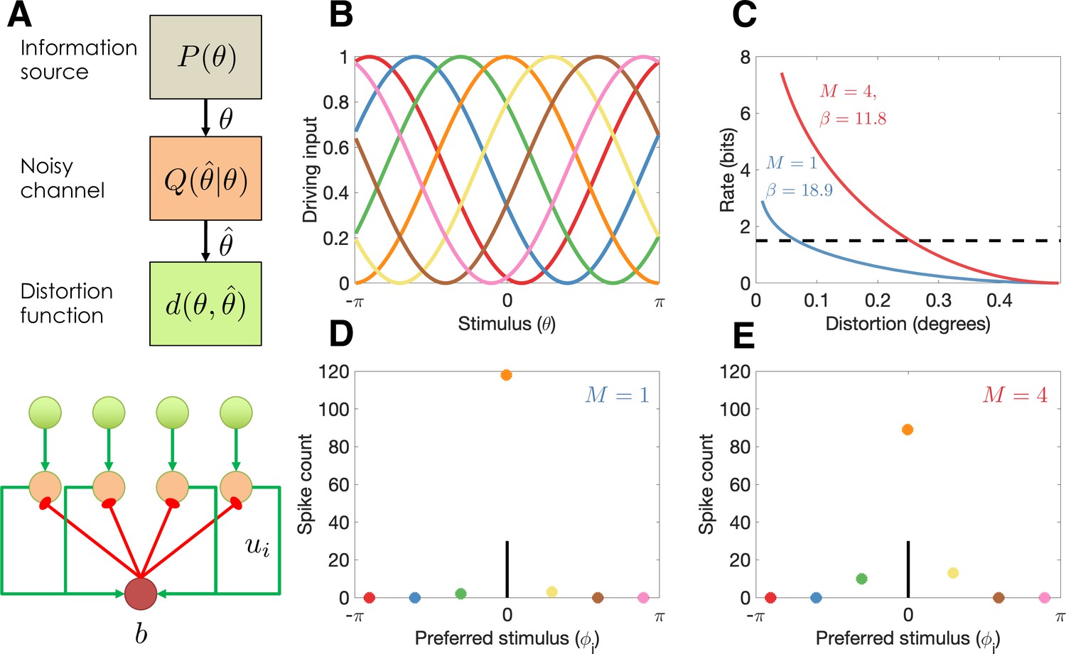
(A) Top: Abstract characterization of a communication channel. A stimulus $θ$ is sampled from an information source $P (θ)$ and passed through a noisy communication channel $Q (\hat{θ} | θ)$ , which outputs a stimulus reconstruction $\hat{θ}$ . The reconstruction error is quantified by a distortion function, $d (θ, \hat{θ})$ . Bottom: Circuit architecture implementing the communication channel. Input neurons encoding the negative distortion function provide the driving input to output neurons with excitatory input u_i and global feedback inhibition $b$ . Each circuit codes a single stimulus at a fixed retinotopic location. When multiple stimuli are presented, the circuits operate in parallel, interacting only through a common gain parameter, $β$ . (B) Tuning curves of input neurons encoding the negative cosine distortion function over a circular stimulus space. (C) Rate-distortion curves for two different set sizes ( $M = 1$ and $M = 4$ ). The optimal gain parameter $β$ is shown for each curve, corresponding to the point at which each curve intersects the channel capacity (horizontal dashed line). Expected distortion decreases with the information rate of the channel, but the channel capacity imposes a lower bound on expected distortion. (D) Example spike counts for output neurons in response to a stimulus ( $θ = 0$ , vertical line). The output neurons are color coded by their corresponding input neuron (arranged horizontally by their preferred stimulus, $ϕ_{i}$ for neuron $i$ ; full tuning curves are shown in panel B). When only a single stimulus is presented ( $M = 1$ ), the gain is high and the output neurons report the true stimulus with high precision. (E) When multiple stimuli are presented $(M = 4)$ , the gain is lower and the output has reduced precision (i.e., sometimes the wrong output neuron fires).

With these elements in hand, we can define the channel design problem as finding the channel $Q^{*}$ that minimizes expected distortion $D \equiv E [d (θ, \hat{θ})]$ subject to the constraint that the information rate $R$ cannot exceed the capacity limit $C$ :

Q^{*} = \underset{Q : R \leq C}{\arg min} D .

For computational convenience, we can equivalently formulate this as an unconstrained optimization problem using a Lagrangian:

Q^{*} = \underset{Q}{\arg min} R + β D,

where $β$ is a Lagrange multiplier equal to the negative slope of the rate-distortion function at the capacity limit:

β = - \frac{\partial R}{\partial D} .

Intuitively, the Lagrangian can be understood as expressing a cost function that captures the need to both minimize distortion (i.e., memory should be accurate) and minimize the information rate (i.e., memory resources should economized). The Lagrange parameter $β$ determines the trade-off between these two terms. Note that because the optimal trade-off function is always monotonically non-increasing and convex, the value of $β$ is always positive and non-increasing in $D$ .

By integrating the ordinary differential equation defined in Equations 2 and 3 and using the Lagrangian formulation, one can show that the optimal channel for a discrete stimulus takes the following form:

Q^{*} (\hat{θ} | θ) \propto \exp [- β d (θ, \hat{θ}) + \log \bar{Q} (\hat{θ})],

where the marginal probability $\bar{Q} (\hat{θ})$ is defined by:

\bar{Q} (\hat{θ}) = \sum_{θ} P (θ) Q^{*} (\hat{θ} | θ) .

These two equations are coupled. One can obtain the optimal channel by initializing them to uniform distributions and iterating them until convergence. This is known as the Blahut–Arimoto algorithm (Blahut, 1972; Arimoto, 1972).

For a channel with a fixed capacity $C$ but variable $D$ across contexts, the Lagrange multiplier $β$ will need to be adjusted for each context so that $R = C$ . We can accomplish this by computing $R$ for a range of $β$ values and choosing the value that gets closest to the constraint $C$ (later we will propose a more biologically plausible algorithm). Intuitively, $β$ characterizes the sensitivity of the channel to the stimulus. When stimulus sensitivity is lower, the information rate is lower and hence the expected distortion is higher.

In general, we will be interested in communicating a collection of $M$ stimuli, $θ = {θ_{1}, \dots, θ_{M}}$ , with associated probing probabilities $π = {π_{1}, \dots, π_{M}}$ , where $π_{m}$ is the probability that stimulus $m$ will be probed (van den Berg and Ma, 2018). The resulting distortion function is obtained by marginalizing over the probe stimulus:

d (θ, \hat{θ}) = \sum_{m} π_{m} d (θ_{m}, {\hat{θ}}_{m}) .

Optimal population coding

We now consider how to realize the optimal channel with a population of spiking neurons, each tuned to a particular stimulus (Figure 1A). The firing rate of neuron $i$ is determined by a simple Spike Response Model (Gerstner and Kistler, 2002) in which the membrane potential is the difference between the excitatory input, u_i, and the inhibitory input, $b$ , which we model as common across neurons (to keep notation simple, we will suppress the time index for all variables). Spiking is generated by a Poisson process, with firing rate modeled as an exponential function of the membrane potential (Jolivet et al., 2006):

r_{i} = \exp [u_{i} - b] .

We assume that inhibition is given by $b = \log \sum_{i} \exp [u_{i}]$ , in which case the firing rate is driven by the excitatory input with divisive normalization (Carandini and Heeger, 2011):

r_{i} = \frac{\exp [u_{i}]}{\sum_{j} \exp [u_{j}]} .

The resulting population dynamics is a form of ‘winner-take-all’ circuit (Nessler et al., 2013). If each neuron has a preferred stimulus $ϕ_{i}$ , then the winner can be understood as the momentary channel output, $\hat{θ} = ϕ_{i}$ whenever neuron $i$ spikes (denoted $z_{i} = 1$ ). The probability that neuron $i$ is the winner within a given infinitesimal time window is:

q (\hat{θ} = ϕ_{i} | θ) = r_{i} .

Importantly, Equation 9 has the same functional form as Equation 4, and the two are equivalent if the excitatory input is given by:

u_{i} = - β d (θ, ϕ_{i}) + w_{i},

where

w_{i} = \log \sum_{θ} q (\hat{θ} = ϕ_{i} | θ) P (θ)

is the log marginal probability of neuron $i$ being selected as the winner. We can see from this expression that the first term in Equation 10 corresponds to the neuron’s stimulus-driven excitatory input and the second term corresponds to the neuron’s excitability. The Lagrange multiplier $β$ plays the role of a gain modulation factor.

The excitability term can be learned through a form of intrinsic plasticity (Nessler et al., 2013), using the following spike-triggered update rule:

Δ w_{i} = η (c \exp [- w_{i}] z_{i} - 1),

where $η$ is a learning rate and $c$ a gain parameter. After a spike ( $z_{i} = 1$ ), the excitability is increased proportionally to the inverse exponential of current excitability. In the absence of a spike, the excitability is decreased by a constant. This learning rule is broadly in agreement with experimental studies (Daoudal and Debanne, 2003; Cudmore and Turrigiano, 2004).

Gain adaptation

We now address how to optimize the gain parameter $β$ . We want the circuit to operate at the set point $R = C$ , where the channel capacity $C$ is understood as some fixed property of the circuit, whereas the information rate $R$ can vary based on the parameters and input distribution, but cannot persistently exceed $C$ . Assuming the total firing rate of the population is approximately constant across time, we can express the information rate as follows:

R = E [\log \frac{Q (\hat{θ} | θ)}{\bar{Q} (\hat{θ})}] = \sum_{i = 1}^{N} \sum_{θ} P (θ) E [\log r_{i} | θ] - E [\log r_{i}],

where $N$ is the number of neurons. This expression reveals that channel capacity corresponds to a constraint on stimulus-driven deviations in firing rate from the marginal firing rate. When the stimulus-driven firing rate is persistently greater than the marginal firing rate, the population may incur an unsustainably large metabolic cost (Levy and Baxter, 1996; Laughlin et al., 1998). When the stimulus-driven firing rate is lower than the marginal firing rate, the population is underutilizing its information transmission resources. We can adapt the deviation through a form of homeostatic plasticity, by increasing $β$ when the deviation is below the channel capacity, and decreasing $β$ when the deviation is above the channel capacity. Concretely, a simple update rule implements this idea:

Δ β = α (C - R),

where $α$ is a learning rate parameter. We assume that this update is applied continuously. A similar adaptive gain modulation has been observed in neural circuits (Desai et al., 1999; Hengen et al., 2013; Hengen et al., 2016). Mechanistically, this could be implemented by changes in background activity: when stimulus-driven excitation is high, the inhibition will also be high (the network is balanced), and the ensuing noise will effectively decrease the gain (Chance et al., 2002).

In this paper, we do not directly model how the information rate $R$ is estimated in a biologically plausible way. One possibility is that this is implemented with slowly changing extracellular calcium levels, which decrease when cells are stimulated and then slowly recover. This mirrors (inversely) the qualitative behavior of the information rate. More quantitatively, it has been posited that the relationship between firing rate and extracellular calcium level is logarithmic (King et al., 2001), consistent with the mathematical definition in Equation 13. Thus, in this model, capacity $C$ corresponds to a calcium set point, and the gain parameter adapts to maintain this set point. A related mechanism has been proposed to control intrinsic excitability via calcium-driven changes in ion channel conductance (LeMasson et al., 1993; Abbott and LeMasson, 1993).

Multiple stimuli

In the case where there are multiple stimuli, the same logic applies, but now we calculate the information rate over all the subpopulations of neurons (each coding a different stimulus). Specifically, the excitatory input becomes:

u_{i m} = - β π_{m} d (θ_{m}, ϕ_{i m}) + w_{i m},

where $m$ indexes both stimuli and separate subpopulations of neurons tuned to each stimulus location (or other stimulus feature that individuates the stimuli). As a consequence, $β$ will tend to be smaller when more stimuli are encoded, because the same capacity constraint will be divided across more neurons.

Memory maintenance

In delayed response tasks, the stimulus is presented transiently, and then probed after a delay. The channel thus needs to maintain stimulus information across the delay. Our model assumes that the excitatory input u_i maintains a trace of the stimulus across the delay. The persistence of this trace is determined by the gain parameter $β$ . Because persistently high levels of stimulus-evoked activity may, according to Equation 13, increase the information rate above the channel capacity, the learning rule in Equation 14 will reduce $β$ and thereby functionally decay the memory trace.

The circuit model does not commit to a particular mechanism for maintaining the stimulus trace. A number of suitable mechanisms have been proposed (Zylberberg and Strowbridge, 2017). One prominent model posits that recurrent connections between stimulus-tuned neurons can implement an attractor network that maintains the stimulus trace as a bump of activity (Wang, 2001; Amit and Brunel, 1997). Other models propose cell-intrinsic mechanisms (Egorov et al., 2002; Durstewitz and Seamans, 2006) or short-term synaptic modifications (Mongillo et al., 2008; Bliss and D’Esposito, 2017). All of these model classes are potentially compatible with the theory that population codes are optimizing a rate-distortion trade-off, provided that the dynamics of the memory trace conform to the equations given above.

During time periods when no memory trace needs to be maintained, such as the intertrial interval (ITI) in delayed response tasks, we assume that the information rate is 0. Because the information rate is the average number of bits communicated across the channel, these ‘silent’ periods effectively increase the achievable information rate during ‘active’ periods (which we denote by $R_{A}$ ). Specifically, if $T_{A}$ is the active time (delay period length), and $T_{S}$ is the silent time (ITI length), then the channel’s rate is given by:

R = \frac{T_{A}}{T_{A} + T_{S}} R_{A} .

Equivalently, we can ignore the intervals in our model and simply rescale the channel capacity by $(T_{A} + T_{S}) / T_{A}$ . This will allow us to model the effects of delay and ITI on performance in working memory tasks.

Implications for working memory

Continuous report with circular stimuli

We apply the framework described above to the setting in which each stimulus is drawn from a circular space (e.g., color or orientation), $θ_{m} \in (- π, π)$ , which we discretize. Reconstruction errors are evaluated using a cosine distortion function:

d (θ, \hat{θ}) = - ω \cos (θ - \hat{θ}),

where $ω > 0$ is a scaling parameter. This implies that the input neurons have cosine tuning curves (Figure 1B), and the output neurons have Von Mises tuning curves, as assumed in previous population coding models of visual working memory for circular stimulus spaces (Bays, 2014; Schneegans and Bays, 2018; Taylor and Bays, 2018; Tomić and Bays, 2018). All of our subsequent simulations use the same tuning curves.

As an illustration of the model behavior in the continuous report task, we compare performance for set sizes 1 and 4. The optimal trade-off curves are shown in Figure 1C. For every point on the curve, the same information rate achieves a lower distortion for set size 1, due to the fact that all of the channel capacity can be devoted to a single stimulus (a hypothetical capacity limit is shown by the dashed horizontal line). In the circuit model, this higher performance is achieved by a narrow bump of population activity around the true stimulus (Figure 1D), compared to a broader bump when multiple stimuli are presented (Figure 1E).

In the following sections, we compare the full rate-distortion model (as described above) with two variants. The ‘fixed gain’ variant assumes that $β$ is held fixed to a constant (fit as a free parameter) rather than adjusted dynamically. The ‘no plasticity’model holds the neural excitability to a fixed value (fit as a free parameter). These two variants remove features of the full rate-distortion model which critically distinguish it from the population coding model of working memory (Bays, 2014). As a strong test of our model, we fit only to data from Experiment 1 in Bays, 2014, and then evaluated the model on the other datasets without fitting any free parameters.

Set size

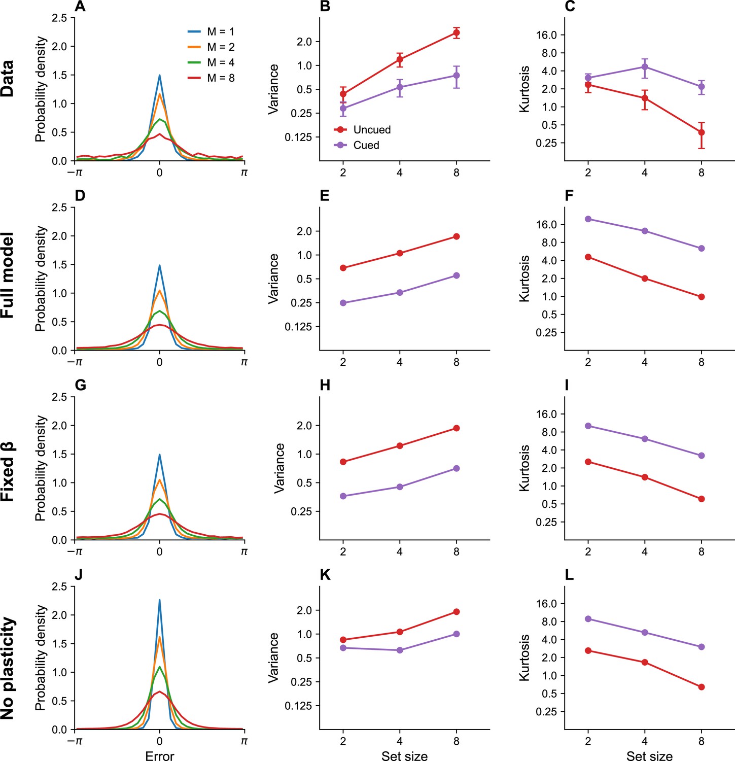
One of the most fundamental findings in the visual working memory literature is that memory precision decreases with set size (Bays et al., 2009; Bays, 2014; Wilken and Ma, 2004). Our model asserts that this is the case because the capacity constraint of the system is divided across more neurons as the number of stimuli to be remembered increases, thus reducing the recall accuracy for any one stimulus. Figure 2A shows the distribution of recall error for different set sizes as published in previous work (Bays, 2014). Figure 2D shows simulation results replicating these findings.

Figure 2

Download asset Open asset

Prioritization

Stimuli that are attentionally prioritized are recalled more accurately. For example, error variance is reduced by a cue that probabilistically predicts the location of the probed stimulus (Bays, 2014; Yoo et al., 2018). In our model, the cue is encoded by the probing probability $π_{m}$ , which alters the expected distortion. This results in greater allocation of the capacity budget to cued stimuli than to uncued stimuli. Figure 2B, C shows empirical findings (variance and kurtosis), which are reproduced by our simulations shown in Figure 2E, F. Kurtosis is one way of quantifying deviation from normality: values greater than 0 indicate tails of the error distribution that are heavier than expected under a normal distribution. The ‘excess’ kurtosis observed in our model is comparable to that observed by Bays in his population coding model (Bays, 2014) when gain is sufficiently low. This is not surprising, given the similarity of the models.

Timing

It is well established that memory performance typically degrades with the RI (Pertzov et al., 2017; Panichello et al., 2019; Schneegans and Bays, 2018; Zhang and Luck, 2009), although the causes of this degradation are controversial (Oberauer et al., 2016), and in some cases the effect is unreliable (Shin et al., 2017). According to our model, this occurs because long RIs tax the information rate of the neural circuit. In order to stay within the channel capacity, the circuit reduces the gain parameter $β$ for long RIs, thereby reducing the information rate and degrading memory performance.

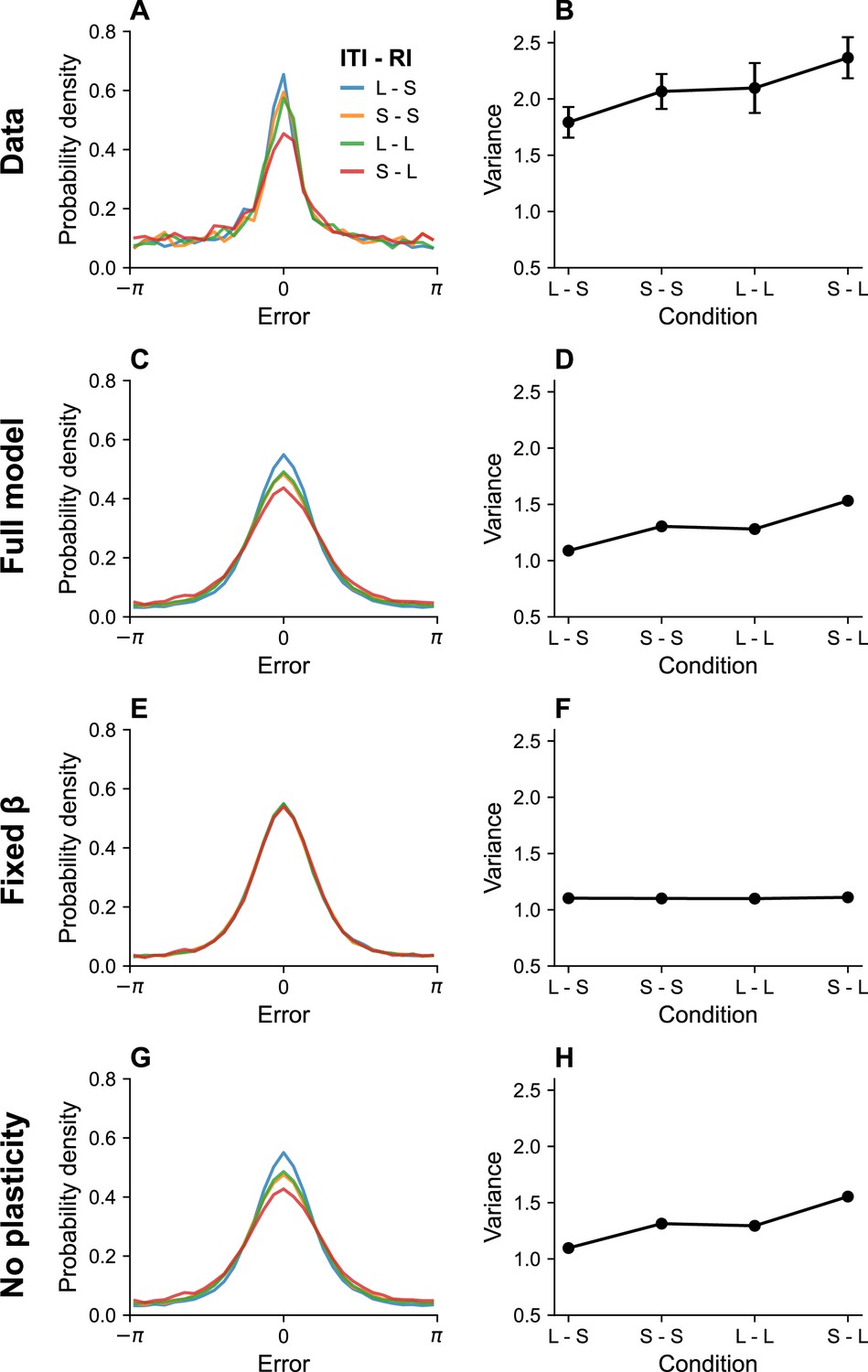
Memory performance also depends on the ITI, but in the opposite direction: longer ITIs improve performance (Souza and Oberauer, 2015; Shipstead and Engle, 2013). The critical determinant of performance is in fact the ratio between the ITI and RI. Souza and Oberauer, 2015 found that performance in a color working memory task was similar when both intervals were short or both intervals were long. They also reported that a longer RI could produce better memory performance when it is paired with a longer ITI. Figure 3 shows a simulation of the same experimental paradigm, reproducing the key results. This timescale invariance, which is also seen in studies of associative learning (Balsam and Gallistel, 2009), arises as a direct consequence of Equation 16. Increasing the ITI reduces the information rate, since no stimuli are being communicated during that time period, and can therefore compensate for longer RIs.

Figure 3

Download asset Open asset

Timing effects.

(A) Error distributions for different intertrial intervals (ITIs) and retention intervals (RIs), as reported in Souza and Oberauer, 2015. ‘S’ denotes a short interval, and ‘L’ denotes a long interval. (B) Error variance as a function of timing parameters. Longer ITIs are associated with lower error variance, whereas longer RIs are associated with larger error variance. Simulation results for the full model (**C, D**), model with fixed gain parameter $β$ (**E, F**), and model without plasticity term $w$ (**G, H**). Error bars represent standard error of the mean.

Serial dependence

Working memory recall is biased by recent stimuli, a phenomenon known as serial dependence (Fischer and Whitney, 2014; Fritsche et al., 2017; Bliss et al., 2017; Papadimitriou et al., 2015). Recall is generally attracted toward recent stimuli, though some studies have reported repulsive effects when the most recent and current stimulus differ by a large amount (Barbosa et al., 2020; Bliss et al., 2017). Our theory explains serial dependence as a consequence of the marginal firing rate of the output cells, which biases the excitatory input u_i (see Equation 10). Because the marginal firing rate is updated incrementally, it will reflect recent stimulus history.

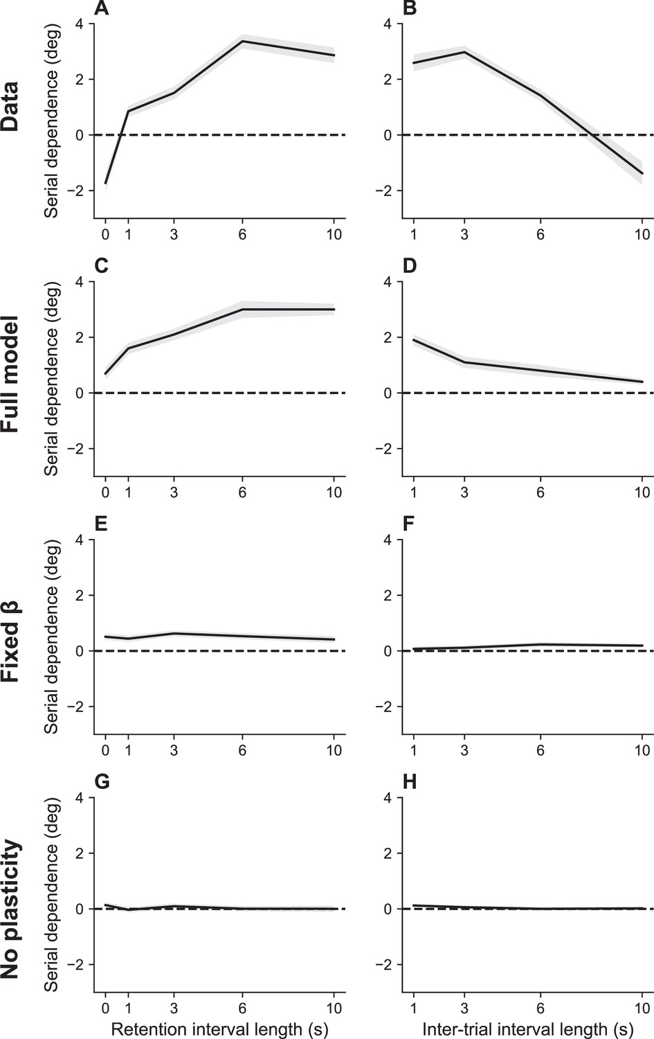
An important benchmark for theories of serial dependence is the finding that it increases with the RI and decreases with ITI (Bliss et al., 2017). These twin dependencies are reproduced by our model (Figure 4). Our explanation of serial dependence is closely related to our explanation of timing effects on recall error: the strength of serial dependence varies inversely with the information rate, which in turn increases with the ITI and decreases with the RI. Mechanistically, this effect is mediated by adjustments of the gain parameter $β$ in order to keep the information rate near the channel capacity.

Figure 4

Download asset Open asset

Serial dependence as a function of retention interval and intertrial interval.

(A) Serial dependence increases with the retention interval until eventually reaching an asymptote, as reported in Bliss et al., 2017. Serial dependence is quantified as the peak-to-peak amplitude of a derivative of Gaussian (DoG) tuning function fitted to the data using least squares (see Methods). (B) Serial dependence decreases with intertrial interval. Simulation results for the full model (**C, D**), model with fixed gain parameter $β$ (**E, F**), and model without plasticity term $w$ (**G, H**). Shaded area corresponds to standard error of the mean.

Serial dependence has also been shown to build up over the course of an experimental session (Barbosa and Compte, 2020). This is hard to explain in terms of theories based on purely short-term effects, but it is consistent with our account in terms of the bias induced by the marginal firing rate. Because this bias reflects continuous incremental adjustments, it integrates over the entire stimulus history, thereby building up over the course of an experimental session (Figure 5).

Figure 5

Download asset Open asset

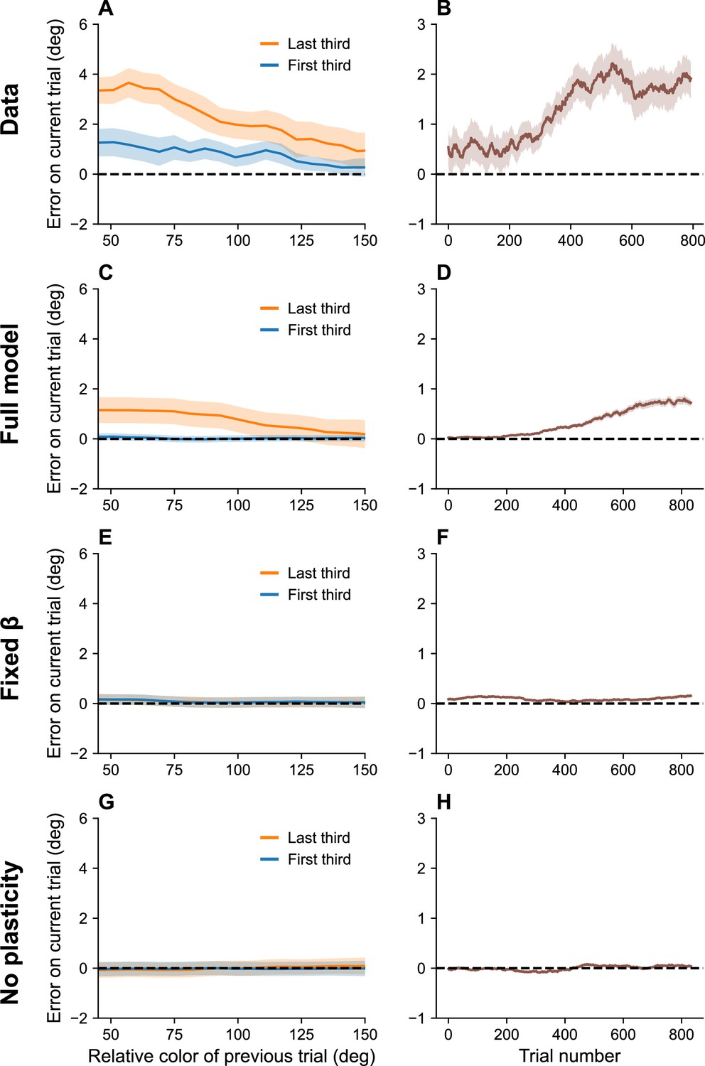
Serial dependence builds up during an experiment.

(A) Serial dependence computed using first third (blue) and last third (orange) of the trials within a session, as reported in Barbosa and Compte, 2020. Data shown here were originally reported in Foster et al., 2017. To obtain a trial-by-trial measure of serial dependence, we calculated the folded error as described in Barbosa and Compte, 2020 (see Methods). Positive values indicate attraction to the last stimulus, while negative values indicate repulsion. Serial dependence is stronger in the last third of the trials in the experiment compared to the first third. (B) Serial dependence increases over the course of the experimental session, computed here with a sliding window of 200 trials. Simulation results for the full model (**C, D**), model with fixed gain parameter $β$ (**E, F**), and model without plasticity term $w$ (**G, H**). Shaded area corresponds to standard error of the mean.

If, as we hypothesize, serial dependence reflects a capacity limit, then we should expect it to increase with set size, since $β$ must decrease to stay within the capacity limit. To the best of our knowledge, this prediction has not been tested. We confirmed this prediction for color working memory using a large dataset reported in Panichello et al., 2019. Figure 6 shows that the attractive bias for similar stimuli on consecutive trials is stronger when the set size is larger (p < 0.05, group permutation test).

Figure 6

Download asset Open asset

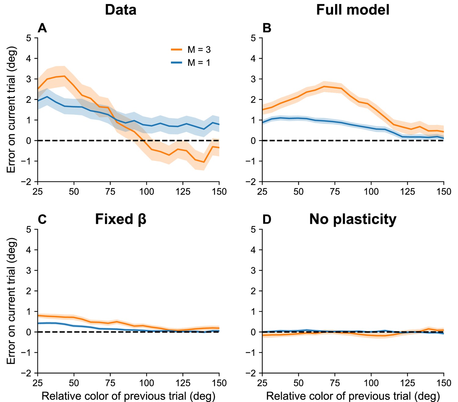
Serial dependence increases with set size.

(A) Serial dependence (quantified using folded error) for set sizes $M = 1$ (blue) and $M = 3$ (orange), using data originally reported in Panichello et al., 2019. Serial dependence computed as the peak amplitude of a derivative of Gaussian (DoG) tuning function fitted to the data using least squares is stronger for larger set sizes (see Methods). On the x-axis, ‘color of previous trial’ refers to the color of the single stimulus probed on the previous trial. (**B–D**) Simulation results for the full model, model with fixed gain parameter $β$ , and model without plasticity term $w$ . Shaded area corresponds to standard error of the mean.

Systematic biases

Working memory exhibits systematic biases toward stimuli that are shown more frequently than others (Panichello et al., 2019). Moreover, these biases increase with the RI, and build up over the course of an experimental session. Our interpretation of serial dependence, which also builds up over the course of a session, suggests that these two phenomena may be linked (see also Tong and Dubé, 2022).

Our theory posits that, over the course of the experiment, the marginal firing rate asymptotically approaches the distribution of presented stimuli (assuming there are no inhomogeneities in the distortion function). Thus, the neurons corresponding to high-frequency stimuli become more excitable than others and bias recall toward their preferred stimuli. This bias is amplified by lower effective capacities brought about by longer RIs. Figure 7 shows simulation results replicating these effects.

Figure 7

Download asset Open asset

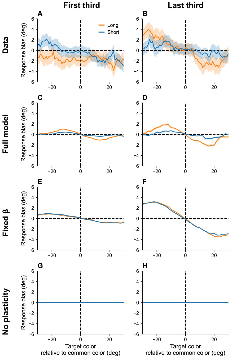
Continuous reports are biased toward high-frequency colors.

(**A, B**) Bias for targets around common colors during the first (Panel A) and last (Panel B) third of the session, as reported in Panichello et al., 2019. Bias refers to the difference between the stimulus and the mean reported color. x-Axis is centered around high-frequency colors. Bias increases with RI length (blue = short RI, orange = long RI). Bias also increases as the experiment progresses. Simulation results for the full model (**C, D**), model with fixed gain parameter $β$ (**E, F**), and model without plasticity term $w$ (**G, H**). Shaded area corresponds to standard error of the mean.

Quantitative model comparison

To systematically compare the performance of the different models, we carried out random-effects Bayesian model comparison (Rigoux et al., 2014) for each dataset (see Methods). This method estimates a population distribution over models from which each subject’s data are assumed to be sampled. The protected exceedance probabilities, shown in Table 1, quantify the posterior probability that each model is the most frequent in the population, taking into account the possibility of the null hypothesis where model probabilities are uniform.

Table 1

Bayesian model comparison between the population coding (PC) model (Bays, 2014), the full rate-distortion (RD), and two variants of the RD model (fixed gain and no plasticity).

Each model is assigned a protected exceedance probability.

Experiment	Figure	PC model	RD model(full)	RD model(fixed gain)	RD model(no plasticity)
Bays, 2014, Experiment 1	2	0.2141	0.2286	0.4128	0.1445
Bays, 2014, Experiment 2	2	0.1853	0.7175	0.0487	0.0485
Souza and Oberauer, 2015	3	0.0115	0.9785	0.0093	0.0007
Bliss and D’Esposito, 2017, Experiment 1	4	0.0000	1.0000	0.0000	0.0000
Bliss et al., 2017, Experiment 2	4	0.0029	0.7689	0.2264	0.0018
Foster et al., 2017	5	0.3185	0.6638	0.0089	0.0088
Panichello et al., 2019, Experiment 1a	6	0.2613	0.7387	0.0000	0.0000
Panichello et al., 2019, Experiment 2	7	0.0544	0.9456	0.0000	0.0000

Experiment 1 from Bays, 2014 did not discriminate strongly between models. All the other datasets provided moderate to strong evidence in favor of the full rate-distortion model, with an average protected exceedance probability of 0.76.

Variations in gain

Equation 14 predicts that operating below the channel capacity will lead to an increase in the gain term $β$ , which, in turn, leads to a higher information rate and better memory performance. Therefore, our model predicts that recall accuracy should improve after a period of poor memory performance, and degrade after a period of good memory performance. At the neural level, the model predicts that error will tend to be lower when gain ( $β$ ) is higher.

We tested these predictions by reanalyzing the monkey neural and behavioral data reported in Barbosa et al., 2020 ( $N = 2$ ). The neural data were collected from the dorsolateral prefrontal cortex, a region classically associated with maintenance of information in working memory (Levy and Goldman-Rakic, 2000; Funahashi, 2006; Wimmer et al., 2014).

Behavioraly, squared error was significantly lower following higher-than-average error than following lower-than-average error (linear mixed model, p < 0.001; Figure 8A), consistent with the hypothesis that gain tends to increase after poor performance and decrease after good performance.

Figure 8

Download asset Open asset

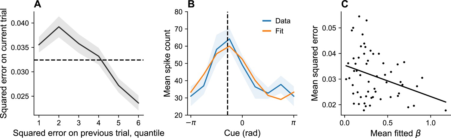
Dynamic variation in memory precision and neural gain.

(A) Mean squared error on current trial, classified by quantiles of squared error on previous trial. Squared error tends to be above average (dashed black line) following low squared error on the previous trial, and tends to be below average following large squared error on the previous trial. (B) Angular location tuning curve (orange) fitted to mean spike count (blue) during the retention interval, shown for one example neuron. The neuron’s preferred stimulus (dashed black line) corresponds to the peak of the tuning curve. Shaded region corresponds to standard error of the mean. (C) Mean squared error for different sessions plotted against mean fitted $β$ . According to our theory, $β$ plays the role of a gain control on the stimulus. Consistent with this hypothesis, memory error decreases with $β$ .

In order to estimate the neural gain, we first inferred the preferred stimulus of each neuron by fitting a bell-shaped tuning function to its spiking behavior (Equation 23, Figure 8B). We then performed Poisson regression to fit a $β$ for each neuron (Equation 24). Model comparison using the Bayesian information criterion (BIC) established that both the distortion function (which captures driving input) and spiking history were significant predictors of spiking behavior (full model: 54,545; no history: 59,163; neither distortion nor history: 67,903). We then examined the relationship between neural gain and memory precision across sessions, finding that session-specific mean squared error was negatively correlated with the average $β$ estimate ( $r$ = –0.32, p < 0.02; Figure 8C). This result is consistent with the hypothesis that dynamic changes in memory performance are associated with changes in neural gain.

Discussion

We have shown that a simple population coding model with spiking neurons can solve the channel design problem: signals passed through the spiking network are transmitted with close to the minimum achievable distortion under the network’s capacity limit. We focused on applying this general model to the domain of working memory, unifying several seemingly disparate aspects of working memory performance: set size effects, stimulus prioritization, serial dependence, approximate timescale invariance, and systematic bias. Our approach builds a bridge between biologically plausible population coding and prior applications of rate-distortion theory to human memory (Sims et al., 2012; Sims, 2015; Sims, 2016; Bates et al., 2019; Bates and Jacobs, 2020; Nagy et al., 2020).

Relationship to other models

The hypothesis that neural systems are designed to optimize a rate-distortion trade-off has been previously studied through the lens of the information bottleneck method (Bialek et al., 2006; Klampfl et al., 2009; Buesing and Maass, 2010; Palmer et al., 2015), a special case of rate-distortion theory in which the distortion function is derived from a compression principle. Specifically, the distortion function is defined as the Kullback–Leibler divergence between $P (θ^{'} | θ)$ and $P (θ^{'} | \hat{θ})$ , where $θ^{'}$ denotes the probed stimulus. This distortion function applies a ‘soft’ penalty to errors based on how much probability mass the channel places on each stimulus. The expected distortion is equal to the mutual information between $θ^{'}$ and $\hat{θ}$ . Thus, the information bottleneck method seeks a channel that maps the input $θ$ into a compressed representation $\hat{θ}$ satisfying the capacity limit, while preserving information necessary to predict the probe $θ^{'}$ .

As pointed out by Leibfried and Braun, 2015, using the Kullback–Leibler divergence as the distortion function leads to a harder optimization compared to classical rate-distortion theory because $P (θ^{'} | \hat{θ})$ depends on the channel distribution, which is the thing being optimized. One consequence of this dependency is that minimizing the rate-distortion objective using alternating optimization (in the style of the Blahut–Arimoto algorithm) is not guaranteed to find the globally optimal channel. It is possible to break the dependency by replacing $P (θ^{'} | \hat{θ})$ with a reference distribution that does not depend on the channel. This turns out to strictly generalize rate-distortion theory, because an arbitrary choice of the reference distribution allows one to recover any lower-bounded distortion function up to a constant offset (Leibfried and Braun, 2015). However, existing spiking neuron implementations of the information bottleneck method (Klampfl et al., 2009; Buesing and Maass, 2010) do not make use of such a reference distribution, and hence do not attain the same level of generality.

Leibfried and Braun, 2015 propose a spiking neuron model that explicitly optimizes the rate-distortion objective function for arbitrary distortion functions. Their approach differs from ours in several ways. First, they model a single neuron, rather than a population. Second, they posit that the channel optimization is realized through synaptic plasticity, in contrast to the intrinsic plasticity rule that we study here. Third, they treat the gain parameter $β$ as fixed, whereas we propose an algorithm for optimizing $β$ .

Open questions

A cornerstone of our approach is the assumption that the neural circuit responsible for working memory dynamically modifies its output to stay within a capacity limit. What, at a biological level, is the nature of this capacity limit? Spiking activity accounts for a large fraction of cortical energy expenditure (Attwell and Laughlin, 2001; Lennie, 2003). Thus, a limit on the overall firing rate of a neural population is a natural transmission bottleneck. Previous work on energy-efficient coding has similarly used the cost of spiking as a constraint (Levy and Baxter, 1996; Stemmler and Koch, 1999; Balasubramanian et al., 2001). One subtlety is that the capacity limit in our framework is an upper bound on the stimulus-driven firing rate relative to the average firing rate (on a log scale). This means that the average firing rate can be high provided the stimulus-evoked transients are small, consistent with the observation that firing rate tends to be maintained around a set point rather than minimized (Desai et al., 1999; Hengen et al., 2013; Hengen et al., 2016). The set point should correspond to the capacity limit.

The next question is how a neural circuit can control its sensitivity to inputs in such a way that the information rate is maintained around the capacity limit. At the single neuron level, this might be realized by adaptation of voltage conductances (Stemmler and Koch, 1999). At the population level, neuromodulators could act as a global gain control. Catecholamines (e.g., dopamine and norepinephrine), in particular, have been thought to play this role (Servan-Schreiber et al., 1990; Durstewitz et al., 1999). Directly relevant to this hypothesis are experiments showing that local injection of dopamine D1 receptor antagonists into the prefrontal cortex impaired performance in an oculomotor delayed response task (Sawaguchi and Goldman-Rakic, 1991), whereas D1 agonists can improve performance (Castner et al., 2000).

In experiments with humans, it has been reported that pharmacological manipulations of dopamine can have non-monotonic effects on cognitive performance, with the direction of the effect depending on baseline dopamine levels (see Cools and D’Esposito, 2011 for a review). The baseline level (particularly in the striatum) correlates with working memory performance (Cools et al., 2008; Landau et al., 2009). Taken together, these findings suggest that dopaminergic neuromodulation controls the capacity limit (possibly through a gain control mechanism), and that pushing dopamine levels beyond the system’s capacity provokes a compensatory decrease in gain, as predicted by our homeostatic model of gain adaptation. A more direct test of our model would use continuous report tasks to quantify memory precision, bias, and serial dependence under different levels of dopamine.

We have considered a relatively restricted range of visual working memory tasks for which extensive data are available. An important open question concerns the generality of our model beyond these tasks. For example, serial order, AX-CPT, and N-back tasks are widely used but outside the scope of our model. With appropriate modification, the rate-distortion framework can be applied more broadly. For example, one could construct channels for sequences rather than individual items, analogous to how we have handled multiple simultaneously presented stimuli. One could also incorporate a capacity-limited attention mechanism for selecting previously presented information for high fidelity representation, rather than storing everything from a fixed temporal window with relatively low fidelity. This could lead to a new information-theoretic perspective on attentional gating in working memory.

Our model can be extended in several other ways. One, as already mentioned, is to develop a biologically plausible implementation of gain adaptation, either through intrinsic or neuromodulatory mechanisms. A second direction is to consider channels that transmit a compressed representation of the input. Previous work has suggested that working memory representations are efficient codes that encode some stimuli with higher precision than others (Koyluoglu et al., 2017; Taylor and Bays, 2018). Finally, an important direction is to enable the model to handle more complex memoranda, such as natural images. Recent applications of large-scale neural networks, such as the variational autoencoder, to modeling human memory hold promise (Nagy et al., 2020; Bates and Jacobs, 2020; Franklin et al., 2020; Bates et al., 2023; Xie et al., 2023), though linking these to more realistic neural circuits remains a challenge.

Methods

We reanalyzed five datasets with human subjects and one dataset with monkey subjects performing delayed response tasks. The detailed experimental procedures can be found in the original reports (Bays, 2014; Souza and Oberauer, 2015; Barbosa et al., 2020; Barbosa and Compte, 2020; Panichello et al., 2019; Bliss and D’Esposito, 2017). In three of the six datasets, one or multiple colors were presented on a screen at equally spaced locations. After an RI, during which the cues were no longer visible, subjects had to report the color at a particular cued location, measured as angles on a color wheel. In one dataset, angled color bars were presented, and the angle of the bar associated with a cued color had to be reported (Bays, 2014). In the two last datasets, only the location of a black cue on a circle had to be remembered and reported (Barbosa et al., 2020; Bliss and D’Esposito, 2017).

Set size and stimulus prioritization

Human subjects ( $N = 7$ ) were presented with 2, 4, or 8 color stimuli at the same time. On each trial, one of the locations was cued before the appearance of the stimuli. Cued locations were 3 times as likely to be probed (Bays, 2014).

We computed trial-wise error as the circular distance between the reported angle and the target angle, separately for each set size and cuing condition. We then calculated circular variance ( $σ^{2}$ ) and kurtosis ( $k$ ) as presented in the original paper, using the following equations:

σ^{2} = - 2 \log | {\bar{m}}_{1} |,

and

k = (| {\bar{m}}_{2} | \cos (Arg ({\bar{m}}_{2}) - 2 Arg ({\bar{m}}_{1})) - | {\bar{m}}_{1} |^{4}) / (1 - | {\bar{m}}_{1} |)^{2},

where ${\bar{m}}_{n}$ is the $n$ th uncentered trigonometric moment. A histogram with $n = 31$ bins was used to visualize the error distribution in Figure 2.

Timing effects

Human subjects ( $N = 36$ ) were presented with 6 simultaneous color stimuli and had to report the color at a probed location as an angle on a color wheel. The RI and ITI lengths varied across sessions (RI: 1 or 3 s, ITI: 1 or 7.5 s) (Souza and Oberauer, 2015). A histogram with $n = 31$ bins was used to visualize the error distribution in Figure 3.

Serial dependence increases with RI and decreases with ITI

Human subjects ( $N = 55$ ) were presented with a black square at a random position on a circle and had to report the location of the cue (Bliss and D’Esposito, 2017). The RI and ITI were varied across blocks of trials (RI: 0, 1, 3, 6, or 10 s, ITI: 1, 3, 6, or 10 s). For each block and subject, we computed serial dependence as the peak-to-peak amplitude of a derivative of Gaussian (DoG) function fit to the data. The DoG function is defined as follows:

y = x a w c \exp (- (w x)^{2}),

where $y$ is the trial-wise error, $x$ is the relative circular distance to the target angle of the previous trial, $a$ is the amplitude of the DoG peak, $w$ is the width of the curve, and $c$ is the constant $\sqrt{2 e}$ , chosen such that the peak-to-peak amplitude of the DoG fit—the measure of serial dependence in Bliss and D’Esposito, 2017—is exactly $2 a$ .

Build-up of serial dependence

Human subjects ( $N = 12$ ) performed a delayed continuous report task with one item (Foster et al., 2017). Following Barbosa and Compte, 2020, we obtained a trial-by-trial measure of serial dependence using their definition of folded error.

Let $θ_{d}$ denotes the circular distance between the angle reported on the previous trial and the target angle on the current trial. In order to aggregate trials with negative $θ_{d}$ (preceding target is located clockwise to current target) and trials with positive $θ_{d}$ (preceding target is located counter-clockwise to current target), we computed the folded error as $θ_{e}^{'} = θ_{e} \times sign (θ_{d})$ , where $θ_{e}$ is the circular distance between the reported angle and the target angle. Positive $θ_{e}^{'}$ corresponds to attraction to the previous stimulus, whereas negative $θ_{e}^{'}$ corresponds to repulsion.

We excluded trials with absolute errors larger than $π / 4$ . We then computed serial bias as the average folded error in sliding windows of width $π / 2$ rad and steps of $π / 30$ rad. We repeated this procedure separately for the trials contained in the first and last third of all sessions. Finally, we computed the increase in serial dependence over the course of a session using a sliding window of 200 trials on the folded error.

Serial dependence increases with set size

We reanalyzed the dataset collected by Panichello et al., 2019, experiment 1a, in which human subjects ( $N = 90$ ) performed a delayed response task with one or three items.

We calculated folded error using the procedure mentioned above. We excluded trials with absolute errors larger than $π / 4$ . We then computed serial bias as the average folded error in sliding windows of width $π / 4$ rad and steps of $π / 30$ rad. We repeated this procedure separately for the trials with $M = 1$ or $M = 3$ items. In order to test whether serial dependence was stronger for one of the set size conditions, we performed a permutation test: We shuffled the entire dataset and partitioned it into two groups of size $S_{M = 1}$ and $S_{M = 3}$ , where $S_{M = m}$ denotes the number of trials recorded for the set size condition $M = m$ . We fitted a DoG curve (Equation 20) to each partition using least squares and computed the difference between the peak amplitude of the two fits. We repeated this process 20,000 times. We then calculated the p-value as the proportion of shuffles for which the difference between the peak amplitudes was equal to or larger than the one computed using the unshuffled dataset.

Continuous reports are biased toward high-frequency colors

Human subjects ( $N = 120$ ) performed a delayed continuous report task with a set size of 2 (Panichello et al., 2019). On each trial, the RI was either 0.5 or 4 s. The stimuli were either drawn from a uniform distribution or from a set of four equally spaced bumps of width $π / 9$ rad with equal probability. The centers of each bump were held constant for each subject.

We defined systematic bias as mean error versus distance to the closest bump center and computed it in sliding windows of width $π / 45$ rad and steps of $π / 90$ rad, as done in the original study. We repeated this procedure separately for the trials with $R I = 0.5 s$ or $R I = 4 s$ , and for the first and last third of trials within a session.

Simulations and model fitting

For each dataset described above, we performed simulations with three different models: the full model, a model with fixed β ( $α = 0$ ), and a model with no plasticity ( $η = 0$ ). The following parameters were held fixed for all simulations, unless stated otherwise: $N = 100$ , $M = 1$ , $ω = 1$ , $η = 10^{- 3}$ , $α = 10^{- 1}$ , $Δ t = 5 \times 10^{- 2}$ s. Weights $w$ were clipped to be in the range $[- 12, 0]$ . β was initialized at $β_{0} = 15$ and clipped to be in the range $[0, 1000]$ .

In order to account for the higher probing probability of the cued stimulus in Bays, 2014, we used

π_{m} = \frac{α_{m}}{\sum_{m^{'}} α_{m^{'}}},

with $α_{priority} = 3$ and $α_{m} = 1$ otherwise, as given by the base rates.

Simulations were run on the same trials as given in the dataset. When multiple stimuli were presented simultaneously ( $M > 1$ ) and the values of non-probed stimuli were not included in the dataset, we used stimuli sampled at random in the range $[- π, π]$ to replace the missing values.

When running a simulation, time was discretized into steps of length $Δ t$ . The simulation time step $Δ t$ was manually set to provide a good trade-off between simulation resolution and run time. The learning rates $η$ and $α$ were scaled by $Δ t$ to make the simulation results largely independent of the precise choice of $Δ t$ . At each step, spikes z_i were generated by sampling from a Poisson distribution with parameter $λ_{i} = \bar{r} r_{i} Δ t$ . Subsequently, w_i, u_i, r_i, $R$ , and $β$ were computed using the equations given in the main text. At the end of the RI, model predictions were performed by decoding samples generated during a window of $T_{d} = 0.1$ s using maximum likelihood estimation.

The capacity $C$ , the population gain $\bar{r}$ , and the plasticity gain parameter $c$ were independently fitted for each subject to maximize the likelihood of the observed errors. To demonstrate the generalizability of these parameter estimates, the parameters were fitted for the dataset from Bays, 2014 only, and then applied without modification to the other datasets. We used the subject-averaged $C$ , $\bar{r}$ , and $c$ to run simulations on the remaining datasets. The one exception was for Souza and Oberauer, 2015, where responses appeared to be unusually noisy responses; for this dataset, we fixed $C = 0.1$ .

In order to compare model performance quantitatively, we fitted the model presented in Bays, 2014 on the dataset presented in the same paper. This model depends on two free parameters: $ω$ , which controls the tuning width of the neurons, and $γ$ , which controls the population gain and corresponds to $\bar{r}$ in our text. These parameters were fit to maximize the likelihood of the observed errors; the detailed model fitting procedure can be found in the original report. As outlined above, averaged parameter estimates were used to run simulations on the remaining datasets. Models were subsequently compared by computing the BIC, defined as:

BIC = k \log (n) - 2 \log (L^{*}),

where $k$ is the number of parameters estimated by the model, $n$ is the number of data points, and $L^{*}$ is the likelihood of the model. For the fitted data, the BIC was used to approximate the marginal likelihood, $P (data) \approx - \frac{1}{2} BIC$ , which was then submitted to the Bayesian model selection algorithm described in Rigoux et al., 2014. Since the same parameters were applied to all the other datasets (i.e., these were generalization tests of the model fit), we instead submitted the log-likelihood directly to Bayesian model selection.

Dynamics of memory precision and neural gain

We reanalyzed the behavioral and neural dataset collected in Barbosa et al., 2020. In this dataset, four adult male rhesus monkeys (Macaca mulatta) were trained in an oculomotor delayed response task that involved fixing their gaze on a central point and subsequently making a saccadic eye movement to the stimulus location after a delay period. While performing the task, firing of neurons in the dorsolateral prefrontal cortex was recorded. Since recordings were not available for all trials within a session, we ignored sessions in which only a subset of the eight potential cues were displayed.

We sorted the squared error on trial $t$ (denoted by $e_{t}^{2}$ ) based on six quantiles of the squared error on the previous trial. We then defined the indicator variable $i_{t} = I (e_{t - 1}^{2} > \bar{e^{2}})$ , taking the value +1 if the squared error on the previous trial was larger than the mean squared error, and −1 otherwise. We then fit the linear mixed model $e_{t}^{2} \sim 1 + i_{t} + (1 | session)$ .

In order to infer the preferred stimulus of each recorded neuron, we used a least squares approach to fit the mean spike count for each presented stimulus and neuron to a bell-shaped tuning function:

f_{i} (θ) = A_{i} \exp (w_{i}^{- 1} (\cos (θ - ϕ_{i}) - 1)),

where $θ$ is the presented stimulus, $A_{i}$ and w_i control the amplitude and width of the tuning function, respectively, and $ϕ_{i}$ is the preferred stimulus of neuron $i$ (Bays, 2014).

We then fitted the neural data by performing Poisson regression for each neuron using the following model:

\log (s_{j}) \sim 1 + D_{j} + {\bar{s}}_{j},

where s_j is the number of spikes emitted by the neuron on trial $j$ , $D_{j}$ is the expected distortion between the stimulus $θ_{j}$ and the neuron’s preferred stimulus, and ${\bar{s}}_{j}$ is an exponential moving average of the neuron’s spike history with decay rate 0.8. We discarded three neurons for which the fitted $β$ was negative and one neuron for which the fitted $β$ was larger than 5 standard deviations above the mean of the fitted values.

In order to ascertain the utility of the different regressors, we fitted another model without the history term, and another without both the distortion and history terms, and compared them based on their BIC values.

Source code

All simulations and analyses were performed using Julia, version 1.6.2. Source code can be found at https://github.com/amvjakob/wm-rate-distortion, (copy archived at Jakob, 2023).

Data availability

The current manuscript is a computational study, so no data have been generated for this manuscript. Source code can be found at https://github.com/amvjakob/wm-rate-distortion (copy archived at Jakob, 2023). The previously published datasets are available upon request from the corresponding authors of the published papers, Souza and Oberauer, 2015, Bliss et al., 2017, and Panichello et al., 2019. A minimally processed dataset from Barbosa et al., 2020 is available online (https://github.com/comptelab/interplayPFC), with the raw data available upon request from the corresponding author of the published paper (raw monkey data available upon request to Christos Constantinidis cconstan@wakehealth.edu, and raw EEG data available upon request to Heike Stein, heike.c.stein@gmail.com). There are no specific application or approval processes involved in requesting these datasets.

The following previously published data sets were used

1. Bays P
(2014) Open Science Framework
ID s7dhn. Noise in Neural Populations Accounts for Errors in Working Memory.

https://osf.io/s7dhn/
1. Foster J
(2017) Open Science Framework
ID vw4uc. Alpha-band activity reveals spontaneous representations of spatial position in visual working memory.

https://osf.io/vw4uc/
1. Barbosa J
(2020) GitHub
ID comptelab/interplayPFC. Interplay between persistent activity and activity-silent dynamics in the prefrontal cortex underlies serial biases in working memory.

https://github.com/comptelab/interplayPFC

References

1. Abbott LF
2. LeMasson G
(1993) Analysis of neuron models with dynamically regulated conductances
Neural Computation 5:823–842.
https://doi.org/10.1162/neco.1993.5.6.823
- Google Scholar
1. Amit DJ
2. Brunel N
(1997) Model of global spontaneous activity and local structured activity during delay periods in the cerebral cortex
Cerebral Cortex 7:237–252.
https://doi.org/10.1093/cercor/7.3.237
- PubMed
- Google Scholar
1. Arimoto S
(1972) An algorithm for computing the capacity of arbitrary discrete memoryless channels
IEEE Transactions on Information Theory 18:14–20.
https://doi.org/10.1109/TIT.1972.1054753
- Google Scholar
1. Attwell D
2. Laughlin SB
(2001) An energy budget for signaling in the grey matter of the brain
Journal of Cerebral Blood Flow and Metabolism 21:1133–1145.
https://doi.org/10.1097/00004647-200110000-00001
- PubMed
- Google Scholar
(2001) Metabolically efficient information processing
Neural Computation 13:799–815.
https://doi.org/10.1162/089976601300014358
- PubMed
- Google Scholar
1. Balsam PD
2. Gallistel CR
(2009) Temporal maps and informativeness in associative learning
Trends in Neurosciences 32:73–78.
https://doi.org/10.1016/j.tins.2008.10.004
- PubMed
- Google Scholar
1. Barbosa J
2. Compte A
(2020) Build-up of serial dependence in color working memory
Scientific Reports 10:10959.
https://doi.org/10.1038/s41598-020-67861-2
- PubMed
- Google Scholar
1. Barbosa J
2. Stein H
3. Martinez RL
4. Galan-Gadea A
5. Li S
6. Dalmau J
7. Adam KCS
8. Valls-Solé J
9. Constantinidis C
10. Compte A
(2020) Interplay between persistent activity and activity-silent dynamics in the prefrontal cortex underlies serial biases in working memory
Nature Neuroscience 23:1016–1024.
https://doi.org/10.1038/s41593-020-0644-4
- PubMed
- Google Scholar
1. Bates CJ
2. Lerch RA
3. Sims CR
4. Jacobs RA
(2019) Adaptive allocation of human visual working memory capacity during statistical and categorical learning
Journal of Vision 19:11.
https://doi.org/10.1167/19.2.11
- PubMed
- Google Scholar
1. Bates CJ
2. Jacobs RA
(2020) Efficient data compression in perception and perceptual memory
Psychological Review 127:891–917.
https://doi.org/10.1037/rev0000197
- PubMed
- Google Scholar
Preprint
(2023) Scaling models of visual working memory to natural images
bioRxiv.
https://doi.org/10.1101/2023.03.17.533050
- Google Scholar
(2009) The precision of visual working memory is set by allocation of a shared resource
Journal of Vision 9:7.
https://doi.org/10.1167/9.10.7
- PubMed
- Google Scholar
1. Bays PM
(2014) Noise in neural populations accounts for errors in working memory
The Journal of Neuroscience 34:3632–3645.
https://doi.org/10.1523/JNEUROSCI.3204-13.2014
- PubMed
- Google Scholar
1. Bays PM
(2015) Spikes not slots: noise in neural populations limits working memory
Trends in Cognitive Sciences 19:431–438.
https://doi.org/10.1016/j.tics.2015.06.004
- PubMed
- Google Scholar
1. Bays PM
(2016) A signature of neural coding at human perceptual limits
Journal of Vision 16:4.
https://doi.org/10.1167/16.11.4
- PubMed
- Google Scholar
Conference
(2006) Efficient representation as a design principle for neural coding and computation
2006 IEEE International Symposium on Information Theory.
https://doi.org/10.1109/ISIT.2006.261867
- Google Scholar
1. Blahut R
(1972) Computation of channel capacity and rate-distortion functions
IEEE Transactions on Information Theory 18:460–473.
https://doi.org/10.1109/TIT.1972.1054855
- Google Scholar
1. Bliss DP
2. D’Esposito M
(2017) Synaptic augmentation in a cortical circuit model reproduces serial dependence in visual working memory
PLOS ONE 12:e0188927.
https://doi.org/10.1371/journal.pone.0188927
- PubMed
- Google Scholar
(2017) Serial dependence is absent at the time of perception but increases in visual working memory
Scientific Reports 7:14739.
https://doi.org/10.1038/s41598-017-15199-7
- PubMed
- Google Scholar
(2009) Compression in visual working memory: using statistical regularities to form more efficient memory representations
Journal of Experimental Psychology. General 138:487–502.
https://doi.org/10.1037/a0016797
- PubMed
- Google Scholar
1. Buesing L
2. Maass W
(2010) A spiking neuron as information bottleneck
Neural Computation 22:1961–1992.
https://doi.org/10.1162/neco.2010.08-09-1084
- PubMed
- Google Scholar
1. Carandini M
2. Heeger DJ
(2011) Normalization as a canonical neural computation
Nature Reviews. Neuroscience 13:51–62.
https://doi.org/10.1038/nrn3136
- PubMed
- Google Scholar
(2000) Reversal of antipsychotic-induced working memory deficits by short-term dopamine D1 receptor stimulation
Science 287:2020–2022.
https://doi.org/10.1126/science.287.5460.2020
- PubMed
- Google Scholar
(2002) Gain modulation from background synaptic input
Neuron 35:773–782.
https://doi.org/10.1016/s0896-6273(02)00820-6
- PubMed
- Google Scholar
(2008) Working memory capacity predicts dopamine synthesis capacity in the human striatum
The Journal of Neuroscience 28:1208–1212.
https://doi.org/10.1523/JNEUROSCI.4475-07.2008
- PubMed
- Google Scholar
1. Cools R
2. D’Esposito M
(2011) Inverted-U-shaped dopamine actions on human working memory and cognitive control
Biological Psychiatry 69:e113–e125.
https://doi.org/10.1016/j.biopsych.2011.03.028
- PubMed
- Google Scholar
1. Cudmore RH
2. Turrigiano GG
(2004) Long-term potentiation of intrinsic excitability in LV visual cortical neurons
Journal of Neurophysiology 92:341–348.
https://doi.org/10.1152/jn.01059.2003
- PubMed
- Google Scholar
1. Daoudal G
2. Debanne D
(2003) Long-term plasticity of intrinsic excitability: learning rules and mechanisms
Learning & Memory 10:456–465.
https://doi.org/10.1101/lm.64103
- PubMed
- Google Scholar
(1999) Plasticity in the intrinsic excitability of cortical pyramidal neurons
Nature Neuroscience 2:515–520.
https://doi.org/10.1038/9165
- PubMed
- Google Scholar
(1999) A neurocomputational theory of the dopaminergic modulation of working memory functions
The Journal of Neuroscience 19:2807–2822.
https://doi.org/10.1523/JNEUROSCI.19-07-02807.1999
- PubMed
- Google Scholar
1. Durstewitz D
2. Seamans JK
(2006) Beyond bistability: biophysics and temporal dynamics of working memory
Neuroscience 139:119–133.
https://doi.org/10.1016/j.neuroscience.2005.06.094
- PubMed
- Google Scholar
(2002) Graded persistent activity in entorhinal cortex neurons
Nature 420:173–178.
https://doi.org/10.1038/nature01171
- PubMed
- Google Scholar
1. Fischer J
2. Whitney D
(2014) Serial dependence in visual perception
Nature Neuroscience 17:738–743.
https://doi.org/10.1038/nn.3689
- PubMed
- Google Scholar
1. Foster JJ
2. Bsales EM
3. Jaffe RJ
4. Awh E
(2017) Alpha-band activity reveals spontaneous representations of spatial position in visual working memory
Current Biology 27:3216–3223.
https://doi.org/10.1016/j.cub.2017.09.031
- PubMed
- Google Scholar
(2020) Structured Event Memory: A neuro-symbolic model of event cognition
Psychological Review 127:327–361.
https://doi.org/10.1037/rev0000177
- PubMed
- Google Scholar
(2017) Opposite effects of recent history on perception and decision
Current Biology 27:590–595.
https://doi.org/10.1016/j.cub.2017.01.006
- PubMed
- Google Scholar
1. Funahashi S
(2006) Prefrontal cortex and working memory processes
Neuroscience 139:251–261.
https://doi.org/10.1016/j.neuroscience.2005.07.003
- PubMed
- Google Scholar
1. Gershman SJ
(2020) Origin of perseveration in the trade-off between reward and complexity
Cognition 204:104394.
https://doi.org/10.1016/j.cognition.2020.104394
- PubMed
- Google Scholar
Book
1. Gerstner W
2. Kistler WM
(2002) Spiking Neuron Models: Single Neurons, Populations, Plasticity.
Cambridge University Press.
https://doi.org/10.1017/CBO9780511815706
- Google Scholar
(2013) Firing rate homeostasis in visual cortex of freely behaving rodents
Neuron 80:335–342.
https://doi.org/10.1016/j.neuron.2013.08.038
- PubMed
- Google Scholar
(2016) Neuronal firing rate homeostasis is inhibited by sleep and promoted by wake
Cell 165:180–191.
https://doi.org/10.1016/j.cell.2016.01.046
- PubMed
- Google Scholar
Software
1. Jakob A
(2023) Wm-rate-distortion, version swh:1:rev:ac3210ae90fb28ef9edc97f0651b3ff3b136eef2
Software Heritage.

https://archive.softwareheritage.org/swh:1:dir:ebc2af8218f6599acf30732c7ad515f5f80d1395;origin=https://github.com/amvjakob/wm-rate-distortion;visit=swh:1:snp:bdcf5343b5f4bf0a42ecd8a701b343673797ff9a;anchor=swh:1:rev:ac3210ae90fb28ef9edc97f0651b3ff3b136eef2
(2006) Predicting spike timing of neocortical pyramidal neurons by simple threshold models
Journal of Computational Neuroscience 21:35–49.
https://doi.org/10.1007/s10827-006-7074-5
- PubMed
- Google Scholar
(2001) Extracellular calcium depletion as a mechanism of short-term synaptic depression
Journal of Neurophysiology 85:1952–1959.
https://doi.org/10.1152/jn.2001.85.5.1952
- PubMed
- Google Scholar
(2017) Serial dependence across perception, attention, and memory
Trends in Cognitive Sciences 21:493–497.
https://doi.org/10.1016/j.tics.2017.04.011
- PubMed
- Google Scholar
(2009) Spiking neurons can learn to solve information bottleneck problems and extract independent components
Neural Computation 21:911–959.
https://doi.org/10.1162/neco.2008.01-07-432
- PubMed
- Google Scholar
(2017) Fundamental bound on the persistence and capacity of short-term memory stored as graded persistent activity
eLife 6:e22225.
https://doi.org/10.7554/eLife.22225
- PubMed
- Google Scholar
1. Lai L
2. Gershman SJ
(2021) Policy compression: An information bottleneck in action selection
Psychology of Learning and Motivation 74:195–232.
https://doi.org/10.1016/bs.plm.2021.02.004
- Google Scholar
1. Landau SM
2. Lal R
3. O’Neil JP
4. Baker S
5. Jagust WJ
(2009) Striatal dopamine and working memory
Cerebral Cortex 19:445–454.
https://doi.org/10.1093/cercor/bhn095
- PubMed
- Google Scholar
(1998) The metabolic cost of neural information
Nature Neuroscience 1:36–41.
https://doi.org/10.1038/236
- PubMed
- Google Scholar
1. Leibfried F
2. Braun DA
(2015) A reward-maximizing spiking neuron as a bounded rational decision maker
Neural Computation 27:1686–1720.
https://doi.org/10.1162/NECO_a_00758
- PubMed
- Google Scholar
(1993) Activity-dependent regulation of conductances in model neurons
Science 259:1915–1917.
https://doi.org/10.1126/science.8456317
- PubMed
- Google Scholar
1. Lennie P
(2003) The cost of cortical computation
Current Biology 13:493–497.
https://doi.org/10.1016/s0960-9822(03)00135-0
- PubMed
- Google Scholar
1. Levy WB
2. Baxter RA
(1996) Energy efficient neural codes
Neural Computation 8:531–543.
https://doi.org/10.1162/neco.1996.8.3.531
- PubMed
- Google Scholar
1. Levy R
2. Goldman-Rakic PS
(2000) Segregation of working memory functions within the dorsolateral prefrontal cortex
Experimental Brain Research 133:23–32.
https://doi.org/10.1007/s002210000397
- PubMed
- Google Scholar
(2008) Synaptic theory of working memory
Science 319:1543–1546.
https://doi.org/10.1126/science.1150769
- PubMed
- Google Scholar
(2020) Optimal forgetting: Semantic compression of episodic memories
PLOS Computational Biology 16:e1008367.
https://doi.org/10.1371/journal.pcbi.1008367
- PubMed
- Google Scholar
(2018) Chunking as a rational strategy for lossy data compression in visual working memory
Psychological Review 125:486–511.
https://doi.org/10.1037/rev0000101
- PubMed
- Google Scholar
(2013) Bayesian computation emerges in generic cortical microcircuits through spike-timing-dependent plasticity
PLOS Computational Biology 9:e1003037.
https://doi.org/10.1371/journal.pcbi.1003037
- PubMed
- Google Scholar
(2016) What limits working memory capacity?
Psychological Bulletin 142:758–799.
https://doi.org/10.1037/bul0000046
- PubMed
- Google Scholar
1. Palmer SE
2. Marre O
3. Berry MJ
4. Bialek W
(2015) Predictive information in a sensory population
PNAS 112:6908–6913.
https://doi.org/10.1073/pnas.1506855112
- PubMed
- Google Scholar
(2019) Error-correcting dynamics in visual working memory
Nature Communications 10:3366.
https://doi.org/10.1038/s41467-019-11298-3
- PubMed
- Google Scholar
(2015) Ghosts in the machine: memory interference from the previous trial
Journal of Neurophysiology 113:567–577.
https://doi.org/10.1152/jn.00402.2014
- PubMed
- Google Scholar
(2017) Rapid forgetting results from competition over time between items in visual working memory
Journal of Experimental Psychology. Learning, Memory, and Cognition 43:528–536.
https://doi.org/10.1037/xlm0000328
- PubMed
- Google Scholar
(2014) Bayesian model selection for group studies - revisited
NeuroImage 84:971–985.
https://doi.org/10.1016/j.neuroimage.2013.08.065
- PubMed
- Google Scholar
1. Sawaguchi T
2. Goldman-Rakic PS
(1991) D1 dopamine receptors in prefrontal cortex: involvement in working memory
Science 251:947–950.
https://doi.org/10.1126/science.1825731
- PubMed
- Google Scholar
1. Schneegans S
2. Bays PM
(2018) Drift in neural population activity causes working memory to deteriorate over time
The Journal of Neuroscience 38:4859–4869.
https://doi.org/10.1523/JNEUROSCI.3440-17.2018
- PubMed
- Google Scholar
(2020) Stochastic sampling provides a unifying account of visual working memory limits
PNAS 117:20959–20968.
https://doi.org/10.1073/pnas.2004306117
- PubMed
- Google Scholar
(1990) A network model of catecholamine effects: gain, signal-to-noise ratio, and behavior
Science 249:892–895.
https://doi.org/10.1126/science.2392679
- PubMed
- Google Scholar
Conference
1. Shannon CE
(1959) Coding theorems for a discrete source with a fidelity criterion
Institute of Radio Engineers, International Convention Record, vol. 7. pp. 325–350.
https://doi.org/10.1109/9780470544242.ch21
- Google Scholar
1. Shin H
2. Zou Q
3. Ma WJ
(2017) The effects of delay duration on visual working memory for orientation
Journal of Vision 17:10.
https://doi.org/10.1167/17.14.10
- PubMed
- Google Scholar
1. Shipstead Z
2. Engle RW
(2013) Interference within the focus of attention: working memory tasks reflect more than temporary maintenance
Journal of Experimental Psychology. Learning, Memory, and Cognition 39:277–289.
https://doi.org/10.1037/a0028467
- PubMed
- Google Scholar
(2012) An ideal observer analysis of visual working memory
Psychological Review 119:807–830.
https://doi.org/10.1037/a0029856
- PubMed
- Google Scholar
1. Sims CR
(2015) The cost of misremembering: Inferring the loss function in visual working memory
Journal of Vision 15:2.
https://doi.org/10.1167/15.3.2
- PubMed
- Google Scholar
1. Sims CR
(2016) Rate-distortion theory and human perception
Cognition 152:181–198.
https://doi.org/10.1016/j.cognition.2016.03.020
- PubMed
- Google Scholar
1. Sims CR
(2018) Efficient coding explains the universal law of generalization in human perception
Science 360:652–656.
https://doi.org/10.1126/science.aaq1118
- PubMed
- Google Scholar
1. Souza AS
2. Oberauer K
(2015) Time-based forgetting in visual working memory reflects temporal distinctiveness, not decay
Psychonomic Bulletin & Review 22:156–162.
https://doi.org/10.3758/s13423-014-0652-z
- PubMed
- Google Scholar
1. Stemmler M
2. Koch C
(1999) How voltage-dependent conductances can adapt to maximize the information encoded by neuronal firing rate
Nature Neuroscience 2:521–527.
https://doi.org/10.1038/9173
- PubMed
- Google Scholar
1. Taylor R
2. Bays PM
(2018) Efficient coding in visual working memory accounts for stimulus-specific variations in recall
The Journal of Neuroscience 38:7132–7142.
https://doi.org/10.1523/JNEUROSCI.1018-18.2018
- PubMed
- Google Scholar
1. Tomić I
2. Bays PM
(2018) Internal but not external noise frees working memory resources
PLOS Computational Biology 14:e1006488.
https://doi.org/10.1371/journal.pcbi.1006488
- PubMed
- Google Scholar
1. Tong K
2. Dubé C
(2022) A tale of two literatures: A fidelity-based integration account of central tendency bias and serial dependency
Computational Brain & Behavior 5:103–123.
https://doi.org/10.1007/s42113-021-00123-0
- Google Scholar
1. van den Berg R
2. Ma WJ
(2018) A resource-rational theory of set size effects in human visual working memory
eLife 7:e34963.
https://doi.org/10.7554/eLife.34963
- PubMed
- Google Scholar
1. Wang XJ
(2001) Synaptic reverberation underlying mnemonic persistent activity
Trends in Neurosciences 24:455–463.
https://doi.org/10.1016/s0166-2236(00)01868-3
- PubMed
- Google Scholar
1. Wilken P
2. Ma WJ
(2004) A detection theory account of change detection
Journal of Vision 4:1120–1135.
https://doi.org/10.1167/4.12.11
- PubMed
- Google Scholar
(2014) Bump attractor dynamics in prefrontal cortex explains behavioral precision in spatial working memory
Nature Neuroscience 17:431–439.
https://doi.org/10.1038/nn.3645
- PubMed
- Google Scholar
Preprint
1. Xie Y
2. Duan Y
3. Cheng A
4. Jiang P
5. Cueva CJ
6. Yang GR
(2023) Natural constraints explain working memory capacity limitations in sensory-cognitive models
bioRxiv.
https://doi.org/10.1101/2023.03.30.534982
- Google Scholar
1. Yoo AH
2. Klyszejko Z
3. Curtis CE
4. Ma WJ
(2018) Strategic allocation of working memory resource
Scientific Reports 8:16162.
https://doi.org/10.1038/s41598-018-34282-1
- PubMed
- Google Scholar
1. Zaslavsky N
2. Kemp C
3. Regier T
4. Tishby N
(2018) Efficient compression in color naming and its evolution
PNAS 115:7937–7942.
https://doi.org/10.1073/pnas.1800521115
- PubMed
- Google Scholar
1. Zhang W
2. Luck SJ
(2009) Sudden death and gradual decay in visual working memory
Psychological Science 20:423–428.
https://doi.org/10.1111/j.1467-9280.2009.02322.x
- PubMed
- Google Scholar
1. Zylberberg J
2. Strowbridge BW
(2017) Mechanisms of persistent activity in cortical circuits: Possible neural substrates for working memory
Annual Review of Neuroscience 40:603–627.
https://doi.org/10.1146/annurev-neuro-070815-014006
- PubMed
- Google Scholar

Decision letter

Paul Bays

Reviewing Editor; University of Cambridge, United Kingdom
Joshua I Gold

Senior Editor; University of Pennsylvania, United States
Paul Bays

Reviewer; University of Cambridge, United Kingdom

Our editorial process produces two outputs: (i) public reviews designed to be posted alongside the preprint for the benefit of readers; (ii) feedback on the manuscript for the authors, including requests for revisions, shown below. We also include an acceptance summary that explains what the editors found interesting or important about the work.

Decision letter after peer review:

Thank you for submitting your article "Rate-distortion theory of neural coding and its implications for working memory" for consideration by eLife. Your article has been reviewed by 3 peer reviewers, including Paul Bays as the Reviewing Editor and Reviewer #1, and the evaluation has been overseen by Joshua Gold as the Senior Editor.

The reviewers have discussed their reviews with one another, and the Reviewing Editor has drafted this to help you prepare a revised submission.

Essential revisions:

1) Expand and clarify the description of the model and how and why it makes the highlighted predictions, to fill in missing steps and make it more comprehensible to readers from a range of backgrounds.

2) Explain to what extent the neural model and its predictions are compatible with neurophysiological observations of stable tuning functions, and the recurrent excitation believed to maintain activity during a delay.

3) Expand the manuscript to better situate the current model in relation to other mechanistic WM models in the literature, and perform quantitative fitting to more concretely evaluate the model's ability to reproduce empirical data. While formal model comparison (e.g. with AIC) may not be necessary, it is important to evaluate the present model's match to data against other models' to understand its relative strengths and weaknesses. As the model is designed to implement an information capacity limit, its ability to reproduce set size effects (on error variability and error distribution) seems worthy of particular attention.

4) Consider and develop the implications of the model's basic principles (e.g. the idea that periods when WM requirement is low can be traded for a boost in information capacity at a later time) for a broader range of WM tasks and observations. This doesn't have to be quantitative fitting but needs to counter the argument that the empirical data currently presented has been selected to fit the model.

Reviewer #1 (Recommendations for the authors):

Some more technical points:

The "simple update rule" of Equation 14 requires knowledge of the information rate R (Equation 13) – is there a plausible method by which this could be computed in the circuit?

WTA, as utilized in the model, is generally a suboptimal decoding method – would predictions change for population vector or ML decoding?

Cosine tuning curves for input neurons lead to von Mises tuning curves for the output neurons – if that's correct it might be worth spelling out as it is the assumed tuning in previous population models of WM.

Excess kurtosis in error distributions has been an important point of debate in WM modelling – it appears to be present in the simulated data, but how does it arise in the model?

How are the smooth "Data" distribution plots generated? Smoothing may be misleading if the shape of the distribution is a question of interest, as it is for set size effects. The smoothing does not appear to take into account the circularity of the response space, based on what happens at π and -pi.

The description of how model predictions are generated needs to be substantially expanded, to explain step-by-step how the data that appears in the "Simulation" panels were produced. How were estimates obtained? How many repetitions/simulated trials were used (the plots are quite noisy)? To what extent were the simulated trials matched to the real ones, in terms of individual stimuli, etc?

What does it mean for the model that the parameter C had to be made ten times smaller for one experiment than the others?

"Spikes contributed to intrinsic synaptic plasticity for 10 timesteps" – what is the implication of this? Is it plausible? Do the results depend on it?

The section on primate data includes results of a model comparison – the methods need to be explained.

Figure 6A axis-label "Relative color of previous trial" – what does this refer to when the set size is three?

The scales in Figure 3B and D don't match.

The variable u_i is in several places (legend of Figure 1, before Equation 15, maybe others) described as the membrane potential instead of excitatory input (which I think is the intended meaning).

Legend of Figure 8B refers to an orientation tuning curve, but I don't believe the task involved oriented stimuli: angular location is probably what is intended.

Figure 1 and elsewhere – using K to indicate set size is going to be very confusing for WM researchers as it has long been used to refer to WM capacity. SS or even N would be preferable.

Reviewer #2 (Recommendations for the authors):

Equation (2): More explanation is needed when moving from the constrained optimization problem to the unconstrained optimization by forming a Lagrangian, especially for some readers of eLife. Add a couple of sentences justifying this step here.

p.3: OK, I'm going to be a bit nitpicky here. "The rate-distortion function is monotonically decreasing" – I'm not sure you can be sure of this. Increasing the capacity could yield no decrease in distortion in some cases (like if you're already at D=0), so technically you should say "monotonically non-increasing" I think. You also say this a couple of paragraphs later to justify \β being decreased, but I think you can only ensure it's non-increasing, I think, but maybe you can convince me otherwise.

Equation (4): Are you just integrating the ODE defined by (2) and (3) to get this result? If so, say that, or give a bit more info on how you arrive at this formula.

"We assume that inhibition is strong enough such that only one neuron in the population will be active within an infinitesimally small time window." – I think this statement is unnecessary. As long as you make a time window small enough, the probability of co-occurring spikes in a window will be zero.

p.6: When you talk about recurrent models, I don't really see any semblance of recurrence in your models. They're just feedforward, right? The weights w_i seem to really just to be inputs. r_i does not feedback into all the other u_j's. Admittedly, this would be a trickier optimization problem to solve using a simple learning rule. Do you have an idea how you would do this if you introduced recurrence into the formulation Equation. (10) and (11)? You could punt this to the Discussion or get into more detail here, but not worrying enough about the mechanism of maintenance of the population spiking means you have to artificially dial down the capacity as the delay time is increased when you get to the "Timing" section on p.9.

Figure 2: You're qualitatively replicating the data, but admittedly missing some details. Variance scales up slower in the model and kurtosis drops off slower. Why? Is this just a case of people satisficing? Also, I think if you follow the analysis in the supplement of Sims et al. (2012), you should be able to get a good analytic approximation of 2D assuming an unbounded (rather than periodic) domain. Even if you place the problem on a periodic domain, I think you can solve the rate-distortion problem by hand to find the correctly parameterized von Mises distribution.

"Increasing the intertrial interval reduces the information rate, since no stimuli are being communicated during that time period, and can therefore compensate for longer retention intervals." – I don't agree with this interpretation. I would think that longer ITIs might lead to less serial bias. Mechanistically, I don't see what else would disrupt persistent activity in a neural circuit as a function of ITI.

p.10: Neural firing rate activity from the previous trial seems an unlikely candidate for the primary mechanism for serial dependence given the persistent activity is typically gone between trials (see Barbosa et al. 2020) – e.g., short-term plasticity or something else seems more likely. I know you're aiming at a parsimonious model, but I think this point warrants discussion.

For all your Simulation/Data comparisons, it's not clear exactly how you chose model parameters. Did you do something systematic to try and best replicate the trends in data? Did you pick an arbitrary \β and stick with this throughout? More and clearer information about this would be helpful.

Reviewer #3 (Recommendations for the authors):

It would be informative to formally compare the current model against alternatives [as one example, Matthey, L., Bays, P. M., and Dayan, P. (2015). A probabilistic palimpsest model of visual short-term memory. PLoS computational biology, 11(1), e1004003.]. As it stands, I am not sure if the model is "yet another model" in a fairly large space, or whether it makes unique predictions or outperforms (or perhaps underperforms) existing models.

Absent formal model comparisons, an extended discussion of the current model's strengths, and especially weaknesses, would greatly improve the manuscript.

[Editors' note: further revisions were suggested prior to acceptance, as described below.]

Thank you for resubmitting your work entitled "Rate-distortion theory of neural coding and its implications for working memory" for further consideration by eLife. Your revised article has been evaluated by Joshua Gold (Senior Editor) and a Reviewing Editor.

The manuscript has been improved, and two out of three reviewers are now satisfied, but there are a small number of remaining issues that need to be addressed, as outlined below:

Reviewer #1 (Recommendations for the authors):

This revision resolves a number of previous concerns, and the clarity of presentation of the model is much improved. There are two issues remaining that I hope can be dealt with relatively straightforwardly:

1. The revision makes clearer where the empirical data, to which the models are compared and fit, comes from, including that the data in Figure 2A corresponds to Exp 1 in ref [15]. However, if that is the case, why is the data from set size 1 missing? Was it also omitted from model fitting? Please remedy this, as predicting recall performance with a single item is pretty crucial for a working memory model.

2. The problems I noted with data smoothing haven't been dealt with. I checked the plots in the original papers corresponding to Figures2 and 3, and its clear the smoothing is strongly distorting the distribution shapes (which form a key part of the evidence the models are intended to reproduce). Is there a reason you can't just plot histograms, like the original papers did for the data?

https://doi.org/10.7554/eLife.79450.sa1

Author response

Essential revisions:

1) Expand and clarify the description of the model and how and why it makes the highlighted predictions, to fill in missing steps and make it more comprehensible to readers from a range of backgrounds.

We’ve now expanded the methods and Results sections to make the model description clearer. Please see responses to the comments below.

2) Explain to what extent the neural model and its predictions are compatible with neurophysiological observations of stable tuning functions, and the recurrent excitation believed to maintain activity during a delay.

As we explain below and on p. 7, we deliberately chose to be agnostic about the memory maintenance mechanism. Several have been proposed in the literature, all of which might be compatible with our framework. The essential constraint imposed by our framework is the capacity limit. Any maintenance mechanism that adheres to this capacity limit is compatible.

We’re not entirely sure what aspect of stable tuning is being referenced here. Some studies suggest representational drift in visual working memory (e.g., Murray et al., 2017; Wolff et al., 2020), so it’s a bit unclear how stable the tuning functions really are. In our setup, the input and output neurons have stable tuning functions; what changes across time is only the gain and excitability.

3) Expand the manuscript to better situate the current model in relation to other mechanistic WM models in the literature, and perform quantitative fitting to more concretely evaluate the model's ability to reproduce empirical data. While formal model comparison (e.g. with AIC) may not be necessary, it is important to evaluate the present model's match to data against other models' to understand its relative strengths and weaknesses. As the model is designed to implement an information capacity limit, its ability to reproduce set size effects (on error variability and error distribution) seems worthy of particular attention.

We now include quantitative model fitting and comparison (summarized in Table 1), both to an existing model (Bays, 2014) and to several variants of the rate-distortion model that lack key features (gain adaptation and intrinsic plasticity).

4) Consider and develop the implications of the model's basic principles (e.g. the idea that periods when WM requirement is low can be traded for a boost in information capacity at a later time) for a broader range of WM tasks and observations. This doesn't have to be quantitative fitting but needs to counter the argument that the empirical data currently presented has been selected to fit the model.

We believe that the standard for breadth should be based on comparable papers in the literature. The most closely related papers to our own are Bays (2014) and Sims (2015). Both of those papers analyzed similar visual working memory tasks (indeed, we analyze some of the same datasets), using similar visual and quantitative metrics. Neither paper attempted to model neurophysiological data, serial dependence, stimulus inhomogeneities, or the effect of intertrial interval timing (some of these were addressed in later papers, though). Given the breadth of findings that are already modeled in our paper, we think that it’s not really a fair assessment to say that we selected data to fit the model. We are in fact trying to explain data that were ignored by many previous models.

We agree that expanding the broader implications of our research is a useful addition. We have done this in a few places. In the “open questions” section of the Discussion (p. 19), we have added the following paragraph:

“In experiments with humans, it has been reported that pharmacological manipulations of dopamine can have non-monotonic effects on cognitive performance, with the direction of the effect depending on baseline dopamine levels (see [83] for a review). The baseline level (particularly in the striatum) correlates with working memory performance [84, 85]. Taken together, these findings suggest that dopaminergic neuromodulation controls the capacity limit (possibly through a gain control mechanism), and that pushing dopamine levels beyond the system’s capacity provokes a compensatory decrease in gain, as predicted by our homeostatic model of gain adaptation. A more direct test of our model would use continuous report tasks to quantify memory precision, bias, and serial dependence under different levels of dopamine.”

Immediately below this paragraph, we have added another new paragraph addressing potential extensions that can address a wider range of tasks:

“We have considered a relatively restricted range of visual working memory tasks for which extensive data are available. An important open question concerns the generality of our model beyond these tasks. For example, serial order, AX-CPT, and N-back tasks are widely used but outside the scope of our model. With appropriate modification, the rate-distortion framework can be applied more broadly. For example, one could construct channels for sequences rather than individual items, analogous to how we have handled multiple simultaneously presented stimuli. One could also incorporate a capacity-limited attention mechanism for selecting previously presented information for high fidelity representation, rather than storing everything from a fixed temporal window with relatively low fidelity. This could lead to a new information-theoretic perspective on attentional gating in working memory.”

Reviewer #1 (Recommendations for the authors):

Some more technical points:

The "simple update rule" of Equation 14 requires knowledge of the information rate R (Equation 13) – is there a plausible method by which this could be computed in the circuit?

This is a great question. We have sketched an answer on p. 6:

“In this paper, we do not directly model how the information rate R is estimated in a biologically plausible way. One possibility is that this is implemented with slowly changing extracellular calcium levels, which decrease when cells are stimulated and then slowly recover. This mirrors (inversely) the qualitative behavior of the information rate. More quantitatively, it has been posited that the relationship between firing rate and extracellular calcium level is logarithmic [40], consistent with the mathematical definition in Equation. 13. Thus, in this model, capacity C corresponds to a calcium set point, and the gain parameter adapts to maintain this set point. A related mechanism has been proposed to control intrinsic excitability via calcium-driven changes in ion channel conductance [41, 42].”

WTA, as utilized in the model, is generally a suboptimal decoding method – would predictions change for population vector or ML decoding?

This is an interesting question, but note that in this case the WTA mechanism is in fact optimal under our specified objective function. We think comparing different decoders would take us too far afield, since our goal was to show how to implement an optimal channel under rate-distortion theory.

Cosine tuning curves for input neurons lead to von Mises tuning curves for the output neurons – if that's correct it might be worth spelling out as it is the assumed tuning in previous population models of WM.

Thanks for pointing this out. We now note this explicitly on p. 7.

Excess kurtosis in error distributions has been an important point of debate in WM modelling – it appears to be present in the simulated data, but how does it arise in the model?

Excess kurtosis was noted by Bays (2014) in his population coding model, but as far as we know there isn’t a naturally intuitive explanation for why this arises from the model. Although we don’t have an intuitive explanation, we’ve elaborated our description of the phenomenon on p. 9:

“Kurtosis is one way of quantifying deviation from normality: values greater than 0 indicate tails of the error distribution that are heavier than expected under a normal distribution. The ‘excess’ kurtosis observed in our model is comparable to that observed by Bays in his population coding model [15] when gain is sufficiently low. This is not surprising, given the similarity of the models.”

How are the smooth "Data" distribution plots generated? Smoothing may be misleading if the shape of the distribution is a question of interest, as it is for set size effects. The smoothing does not appear to take into account the circularity of the response space, based on what happens at π and -pi.

For Figures 2 and 3, we used a kernel density estimate plot to visualize the smoothed data distribution. We used the Python function `kdeplot` from the `seaborn` package with the default parameters.

For Figures 5, 6, 7, we obtained the smoothed data distribution plots by moving window averaging. The precise smoothing parameters we used are given in the Methods. While smoothing the data distribution might introduce artifacts on the edges of the plot domain, the rest of the plot is unaffected for sufficiently light smoothing.

The description of how model predictions are generated needs to be substantially expanded, to explain step-by-step how the data that appears in the "Simulation" panels were produced. How were estimates obtained? How many repetitions/simulated trials were used (the plots are quite noisy)? To what extent were the simulated trials matched to the real ones, in terms of individual stimuli, etc?

We have clarified the model prediction procedure in a step-by-step fashion on p. 22. Furthermore, in the revised version of this manuscript, the simulated trials exactly correspond to the trials in the dataset. While the investigated datasets always contained information on the probed stimulus, in the case of multiple simultaneous stimuli the value of non-probed stimuli were sometimes omitted. In such cases, the missing values were replaced with stimuli sampled at random in the range [-pi, pi].

What does it mean for the model that the parameter C had to be made ten times smaller for one experiment than the others?

As we now clarify in the paper, this particular dataset appears to contain unusually noisy responses, which might be due to several factors, such as the task being more challenging or the subjects being less attentive. Therefore, in order to reasonably fit the dataset, we lowered the model gain. This modeling choice is obviously ad hoc, but hopefully it is justified based on the adequacy of the model fit.

"Spikes contributed to intrinsic synaptic plasticity for 10 timesteps" – what is the implication of this? Is it plausible? Do the results depend on it?

Our results don’t depend strongly on this assumption, and it has been removed from the manuscript. In the revised model, a spike contributes to intrinsic plasticity for one timestep only, the timestep during which it was generated.

The section on primate data includes results of a model comparison – the methods need to be explained.

We have expanded the methods section on primate data analysis, including information on the source of the neural recordings in addition to details of model comparison.

Figure 6A axis-label "Relative color of previous trial" – what does this refer to when the set size is three?

Despite showing three cues, only one is probed during each trial. In this context, “relative color of previous trial” refers to the color of the cue that was probed on the previous trial. We now state this explicitly in the caption.

The scales in Figure 3B and D don't match.

Thank you for pointing this out; it has been corrected.

The variable u_i is in several places (legend of Figure 1, before Equation 15, maybe others) described as the membrane potential instead of excitatory input (which I think is the intended meaning).

Thanks for catching that error; we’ve corrected it throughout.

Legend of Figure 8B refers to an orientation tuning curve, but I don't believe the task involved oriented stimuli: angular location is probably what is intended.

Corrected.

Figure 1 and elsewhere – using K to indicate set size is going to be very confusing for WM researchers as it has long been used to refer to WM capacity. SS or even N would be preferable.

We’ve changed “K” to “M” throughout.

Reviewer #2 (Recommendations for the authors):

Equation (2): More explanation is needed when moving from the constrained optimization problem to the unconstrained optimization by forming a Lagrangian, especially for some readers of eLife. Add a couple of sentences justifying this step here.

We’ve added several sentences around Equation. 2 to hopefully make this more accessible.

p.3: OK, I'm going to be a bit nitpicky here. "The rate-distortion function is monotonically decreasing" – I'm not sure you can be sure of this. Increasing the capacity could yield no decrease in distortion in some cases (like if you're already at D=0), so technically you should say "monotonically non-increasing" I think. You also say this a couple of paragraphs later to justify \β being decreased, but I think you can only ensure it's non-increasing, I think, but maybe you can convince me otherwise.

We’ve changed “decreasing” to “non-increasing” in both places.

Equation (4): Are you just integrating the ODE defined by (2) and (3) to get this result? If so, say that, or give a bit more info on how you arrive at this formula.

We are indeed integrating the ODE defined by Eqs. 2 and 3 to obtain Equation. 4. We have clarified this on p. 22.

"We assume that inhibition is strong enough such that only one neuron in the population will be active within an infinitesimally small time window." – I think this statement is unnecessary. As long as you make a time window small enough, the probability of co-occurring spikes in a window will be zero.

We have removed this sentence.

p.6: When you talk about recurrent models, I don't really see any semblance of recurrence in your models. They're just feedforward, right? The weights w_i seem to really just to be inputs. r_i does not feedback into all the other u_j's. Admittedly, this would be a trickier optimization problem to solve using a simple learning rule. Do you have an idea how you would do this if you introduced recurrence into the formulation Equation. (10) and (11)? You could punt this to the Discussion or get into more detail here, but not worrying enough about the mechanism of maintenance of the population spiking means you have to artificially dial down the capacity as the delay time is increased when you get to the "Timing" section on p.9.

We only mention recurrent networks as one possible model that realizes persistent activation (on p. 7 we discuss other possibilities). We didn’t want to commit to a particular implementation because our theoretical framework is largely agnostic with respect to this choice (this is arguably true of the Bays 2014 population coding model as well).

Note that we did not artificially dial down the capacity as the delay time increases. The gain parameter is endogenously set by Equation. 14. Critically, capacity is assumed to stay fixed across time (we treat this as a physical/structural property of the memory system). As explained in the “memory maintenance” section, interval dependence arises from the fact that a fixed capacity is allocated (typically evenly) across a given interval.

Figure 2: You're qualitatively replicating the data, but admittedly missing some details. Variance scales up slower in the model and kurtosis drops off slower. Why? Is this just a case of people satisficing? Also, I think if you follow the analysis in the supplement of Sims et al. (2012), you should be able to get a good analytic approximation of 2D assuming an unbounded (rather than periodic) domain. Even if you place the problem on a periodic domain, I think you can solve the rate-distortion problem by hand to find the correctly parameterized von Mises distribution.

With respect to the figure, it’s true that we are missing some details, but in our view the differences between model and data are rather subtle.

The analysis suggestion is intriguing, but we felt that it is outside the scope of our paper, which tries to follow closely the setup of Bays (2014), which assumed a periodic domain.

"Increasing the intertrial interval reduces the information rate, since no stimuli are being communicated during that time period, and can therefore compensate for longer retention intervals." – I don't agree with this interpretation. I would think that longer ITIs might lead to less serial bias. Mechanistically, I don't see what else would disrupt persistent activity in a neural circuit as a function of ITI.

Maybe there is some confusion here? The data show that longer ITIs reduce serial dependence, and we reproduce this with our model. So we’re not sure what the point of disagreement is.

p.10: Neural firing rate activity from the previous trial seems an unlikely candidate for the primary mechanism for serial dependence given the persistent activity is typically gone between trials (see Barbosa et al. 2020) – e.g., short-term plasticity or something else seems more likely. I know you're aiming at a parsimonious model, but I think this point warrants discussion.

To be clear, we are not suggesting that the model is updating the gain parameter on a trial-by-trial basis. Rather, Equation. 14 is being applied continuously (which we now state explicitly). So there is no need to assume that persistent activity is maintained between trials.

For all your Simulation/Data comparisons, it's not clear exactly how you chose model parameters. Did you do something systematic to try and best replicate the trends in data? Did you pick an arbitrary \β and stick with this throughout? More and clearer information about this would be helpful.

Thanks for this suggestion. We have now completely redone the modeling using fitted parameters. Our model fitting procedures are described in the Methods (p. 22).

Reviewer #3 (Recommendations for the authors):

It would be informative to formally compare the current model against alternatives [as one example, Matthey, L., Bays, P. M., and Dayan, P. (2015). A probabilistic palimpsest model of visual short-term memory. PLoS computational biology, 11(1), e1004003.]. As it stands, I am not sure if the model is "yet another model" in a fairly large space, or whether it makes unique predictions or outperforms (or perhaps underperforms) existing models.

This is a very interesting model of visual working memory. However, it is primarily focused on memory for multi-feature items, a topic that we don’t address in this paper. While the binding problem in memory is extremely important, we felt that it was outside the scope of this paper, especially given that we are comparing our model to several others already.

Absent formal model comparisons, an extended discussion of the current model's strengths, and especially weaknesses, would greatly improve the manuscript.

Agreed, which is why now we include formal model comparison, summarized in Table 1 and discussed on p. 14.

[Editors' note: further revisions were suggested prior to acceptance, as described below.]

The manuscript has been improved, and two out of three reviewers are now satisfied, but there are a small number of remaining issues that need to be addressed, as outlined below:

Reviewer #1 (Recommendations for the authors):

This revision resolves a number of previous concerns, and the clarity of presentation of the model is much improved. There are two issues remaining that I hope can be dealt with relatively straightforwardly:

1. The revision makes clearer where the empirical data, to which the models are compared and fit, comes from, including that the data in Figure 2A corresponds to Exp 1 in ref [15]. However, if that is the case, why is the data from set size 1 missing? Was it also omitted from model fitting? Please remedy this, as predicting recall performance with a single item is pretty crucial for a working memory model.

Thank you for raising this point. We included the data from set size 1 in the model fitting; we merely omitted plotting it in Figure 2A for visual consistency with Figure 2BC, which uses the dataset from Exp 2 in ref [15], for which only set sizes 2, 4 and 8 are available.

We have now additionally plotted the data and simulation results pertaining to set size 1 in Figure 2A,D,G,J.

2. The problems I noted with data smoothing haven't been dealt with. I checked the plots in the original papers corresponding to Figures2 and 3, and its clear the smoothing is strongly distorting the distribution shapes (which form a key part of the evidence the models are intended to reproduce). Is there a reason you can't just plot histograms, like the original papers did for the data?

We initially smoothed the error distribution plots to remove sampling noise from the simulation results. However, as rightfully noted, this was distorting the distribution shape, especially at the boundaries of the function domain.

We have remedied this matter by plotting histograms instead for both the original data and the simulation results in Figure 2 and Figure 3.

https://doi.org/10.7554/eLife.79450.sa2

Article and author information

Author details

Anthony MV Jakob
1. Section of Life Sciences Engineering, École Polytechnique Fédérale de Lausanne, Lausanne, Switzerland
2. Department of Neurobiology, Harvard Medical School, Boston, United States
Contribution
Conceptualization, Resources, Data curation, Software, Formal analysis, Funding acquisition, Investigation, Visualization, Methodology, Writing – original draft, Writing – review and editing

For correspondence
anthony.jakob@outlook.com

Competing interests
No competing interests declared

"This ORCID iD identifies the author of this article:" 0000-0002-0996-1356
Samuel J Gershman
1. Department of Psychology and Center for Brain Science, Harvard University, Cambridge, United States
2. Center for Brains, Minds, and Machines, MIT, Cambridge, United Kingdom
Contribution
Conceptualization, Resources, Supervision, Funding acquisition, Validation, Methodology, Writing – original draft, Project administration, Writing – review and editing

Competing interests
No competing interests declared

"This ORCID iD identifies the author of this article:" 0000-0002-6546-3298

Funding

Fondation Bertarelli (Bertarelli Fellowship)

Anthony MV Jakob

National Science Foundation (NSF STC award CCF-1231216)

Samuel J Gershman

The funders had no role in study design, data collection, and interpretation, or the decision to submit the work for publication.

Acknowledgements

Johannes Bill, Wulfram Gerstner, and Chris Bates generously provided constructive feedback and discussion. This research was supported by a Bertarelli Fellowship and by the Center for Brains, Minds, and Machines (funded by NSF STC award CCF-1231216).

Senior Editor

Joshua I Gold, University of Pennsylvania, United States

Reviewing Editor

Paul Bays, University of Cambridge, United Kingdom

Reviewer

Paul Bays, University of Cambridge, United Kingdom

Version history

Preprint posted: March 2, 2022 (view preprint)
Received: April 13, 2022
Accepted: June 22, 2023
Accepted Manuscript published: July 12, 2023 (version 1)
Version of Record published: July 18, 2023 (version 2)

Copyright

This article is distributed under the terms of the Creative Commons Attribution License, which permits unrestricted use and redistribution provided that the original author and source are credited.