Data-driven, participatory characterization of farmer varieties discloses teff breeding potential under current and future climates
- Center of Plant Sciences, Scuola Superiore Sant'Anna, Italy
- Amhara Regional Agricultural Research Institute, Ethiopia
- Digital Inclusion, Bioversity International, France
- Department of Agricultural Sciences, Inland Norway University of Applied Sciences, Norway
- Biodiversity for Food and Agriculture, Bioversity International, Kenya
Figures
Figure 1 with 6 supplements
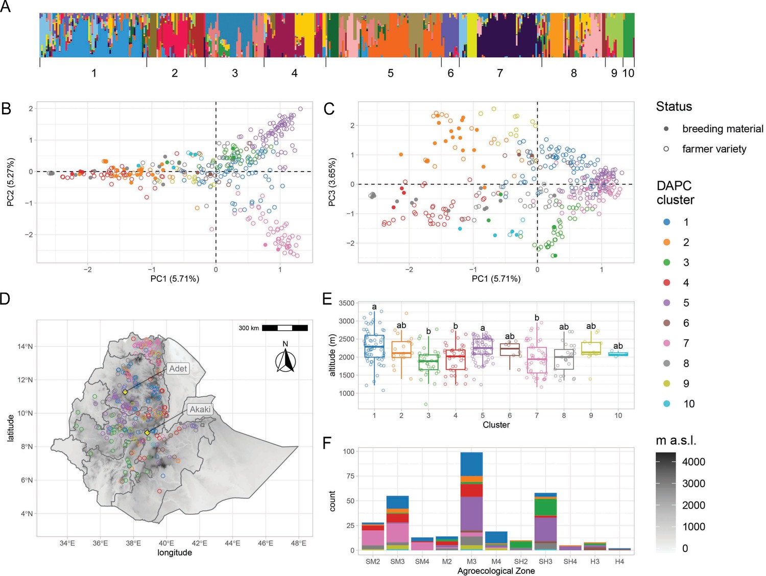
Genetic diversity of teff in Ethiopia.
(A) ADMIXTURE results for the pruned single-nucleotide polymorphisms (SNPs) dataset. Each vertical bar represents an individual, colored according to one of the 20 groups reported by the analysis. Bars are ordered according to the 10 genetic clusters identified by discriminant analysis of principal component (DAPC), as reported by numbers on the x-axis. (B, C) Principal component analysis of genome-wide SNPs. Taxa are colored according to their DAPC genetic cluster, as indicated in the legend. About 10.98% of the genetic diversity in the panel can be explained by the first two principal components, which clearly separate cluster 7 from clusters 2 and 4. Open and close circles represent farmer varieties and improved varieties, respectively. (D) Distribution of Ethiopian Teff Diversity Panel (EtDP) georeferenced landraces (N = 314) across the altitudinal map of Ethiopia, color coded as in panel (B). (E) Altitude distribution across the DAPC genetic clusters,, with letters on top of boxplots denoting significance levels based on a pairwise Wilcoxon rank sum test and Bonferroni correction for multiple testing. (F) Distribution of genetic clusters across agroecological zones of Ethiopia, with color coding as in panel B. SM2, warm submoist lowlands; SM3, tepid submoist mid-highlands; SM4, cool submoist mid-highlands; M2, warm moist lowlands; M3, tepid moist mid-highlands; M4, cool moist mid-highlands; SH2, warm subhumid lowlands; SH3, tepid suphumid mid-highlands; SH4, cool subhumid mid-highlands; H3, tepid humid mid-highlands; H4, cool humid mid-highlands. This figure has six figure supplements.
Figure 1—figure supplement 1
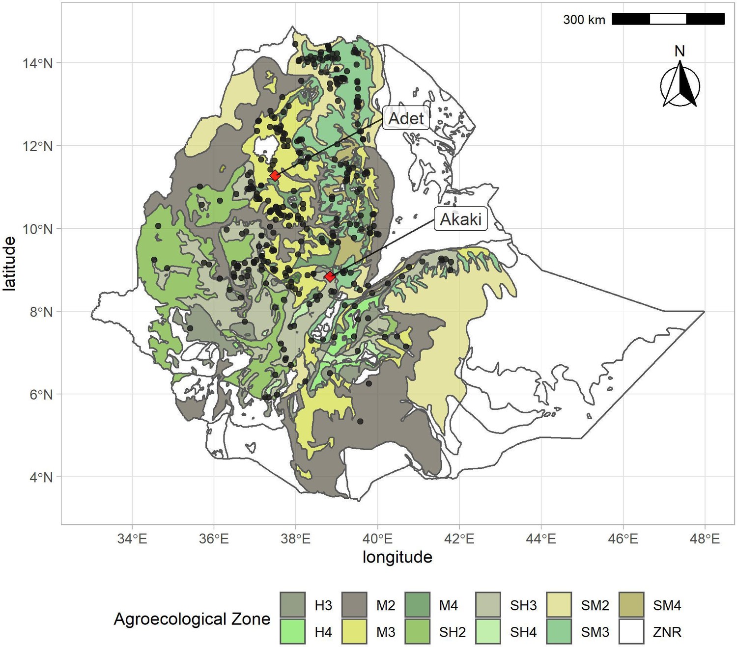
Distribution of georeferenced farmer varieties in the Ethiopian Teff Diversity Panel (EtDP) (N = 314) overlaid to agroecological zones of Ethiopia.
Sampling locations are indicated with black points. Adet and Akaki, the two field experiment sites, are indicated with red diamonds. H3, tepid humid mid-highlands; H4, cool humid mid-highlands; M2, warm moist lowlands; M3, tepid moist mid-highlands; M4, cool moist mid-highlands; SH2, warm subhumid lowlands; SH3, tepid subhumid mid-highlands; SH4, cool subhumid mid-highlands; SM2, warm submoist lowlands; SM3, tepid submoist mid-highlands; SM4, cool submoist mid-highlands; ZNR, zone not relevant (no hits in the teff collection).
Figure 1—figure supplement 2

Linkage disequilibrium (LD) in subgenome A (A) and subgenome B (B).
Each panel shows LD evolution in the 10 chromosomes of each subgenome, from number 1 to the top to number 10 to the bottom. The lines represent r2 values as a rolling window across the chromosome and are colored according to legend. Black triangles represent centromeres. The inset represents LD decay as a function of physical distance of markers. Mb, million basepairs.
Figure 1—figure supplement 3

Predictive accuracy of the model-based unsupervised clustering (ADMIXTURE) and the discriminant analysis of principal components (DAPC) using the fivefold cross-validation procedure and the Bayesian information criterion (BIC), respectively.
(A) Cross-validation (CV) error for Admixture clusters ranging from K = 2 to K = 25. (B) BIC values for different values of DAPC clusters. The optimal number of clusters is 10.
Figure 1—figure supplement 4

Unrooted neighbor-joining phylogenetic trees of the Ethiopian Teff Diversity Panel (EtDP) (N = 366).
Taxa are color coded according to their status, as in the legend.
Figure 1—figure supplement 5
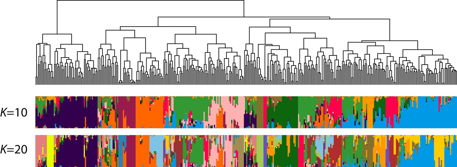
Population structure of the EtDP (N = 366).
The dendrogram represents the result of IBS-based hierarchical clustering analysis. Each individual is represented by a vertical bar, colored according to its belonging to one of the predicted clusters. The two bar plots represent ADMIXTURE assignments for a value of K = 10 (corresponding to the best discriminant analysis of principal component [DAPC] interpretation) and K = 20. Accessions on the x-axis are ordered according to the dendrogram on top.
Figure 1—figure supplement 6
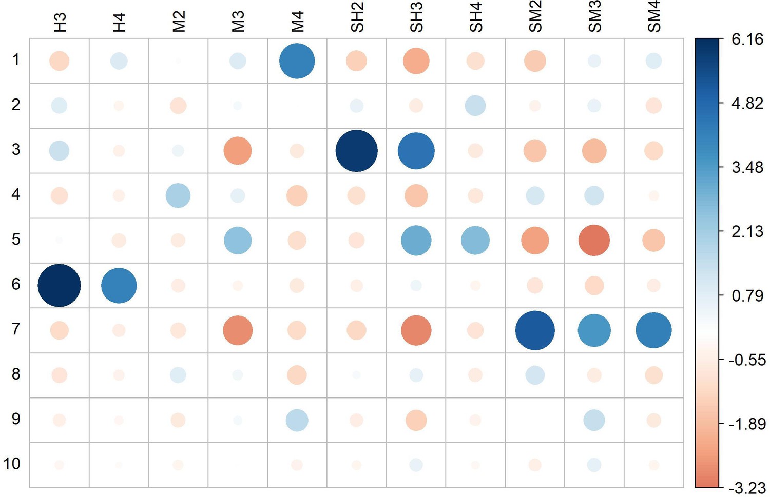
Residual plot for the Pearson’s chi-squared test of independence between discriminant analysis of principal component (DAPC) genetic clusters and Ethiopian agroecological zones (df = 60, p value <2.2e−16).
Circle colors and sizes indicate the relative contribution of each cell to the chi-square score. Dark blue and larger circles indicate higher effect sizes. H3, tepid humid mid-highlands; H4, cool humid mid-highlands; M2, warm moist lowlands; M3, tepid moist mid-highlands; M4, cool moist mid-highlands; SH2, warm subhumid lowlands; SH3, tepid subhumid mid-highlands; SH4, cool subhumid mid-highlands; SM2, warm submoist lowlands; SM3, tepid submoist mid-highlands; SM4, cool submoist mid-highlands; ZNR, zone not relevant (no hits in the teff collection).
Figure 2 with 2 supplements
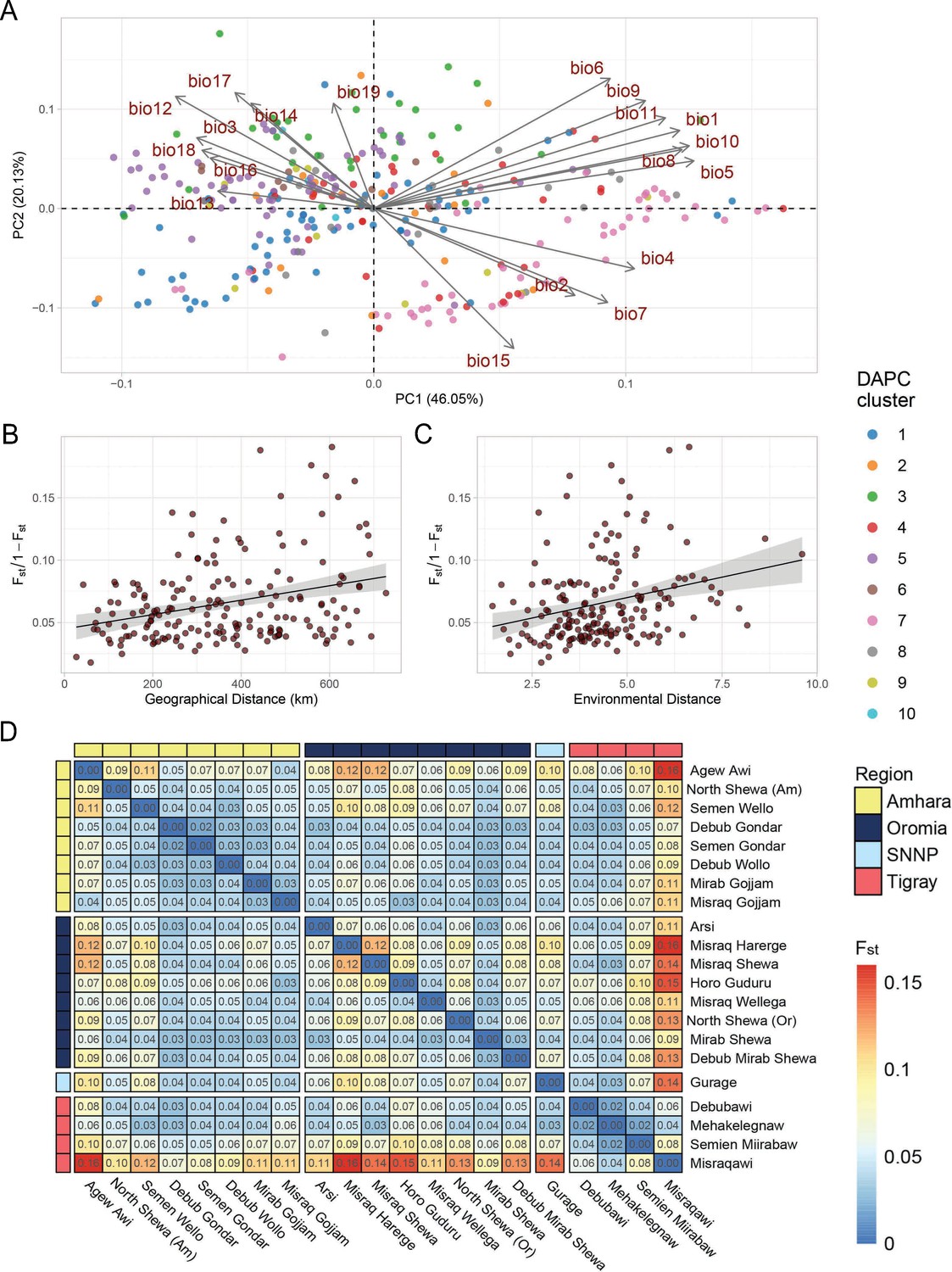
Teff diversity on the landscape.
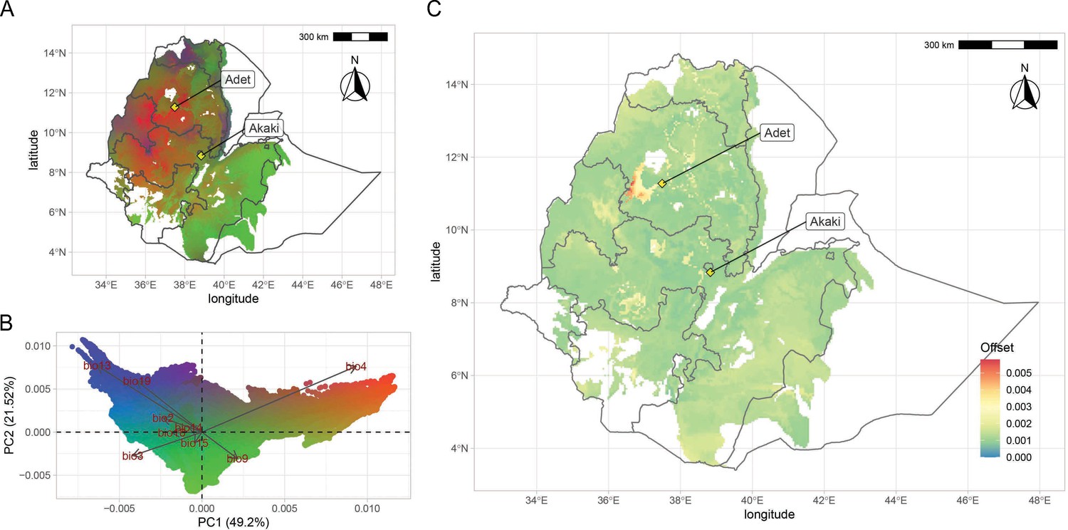
(A) Principal component analysis of bioclimatic diversity in the Ethiopian Teff Diversity Panel (EtDP). Dots represent teff farmer varieties belonging to genetic clusters, colored according to legend. Vectors represent the scale, verse, and direction of bioclimatic drivers of teff differentiation. (B) Linear regression of Fst values in relation to geographic distance of accessions in the EtDP. Accessions were grouped by local district of sampling. (C) Linear regression of Fst values in relation to environmental distance of accessions, also grouped by district of sampling. (D) Pairwise Fst values between teff accessions grouped by local districts of sampling, as in (C) and (D). Local districts, that is subregional groups, are ordered by administrative regions according to legend. This figure has two figure supplements.
Figure 2—figure supplement 1
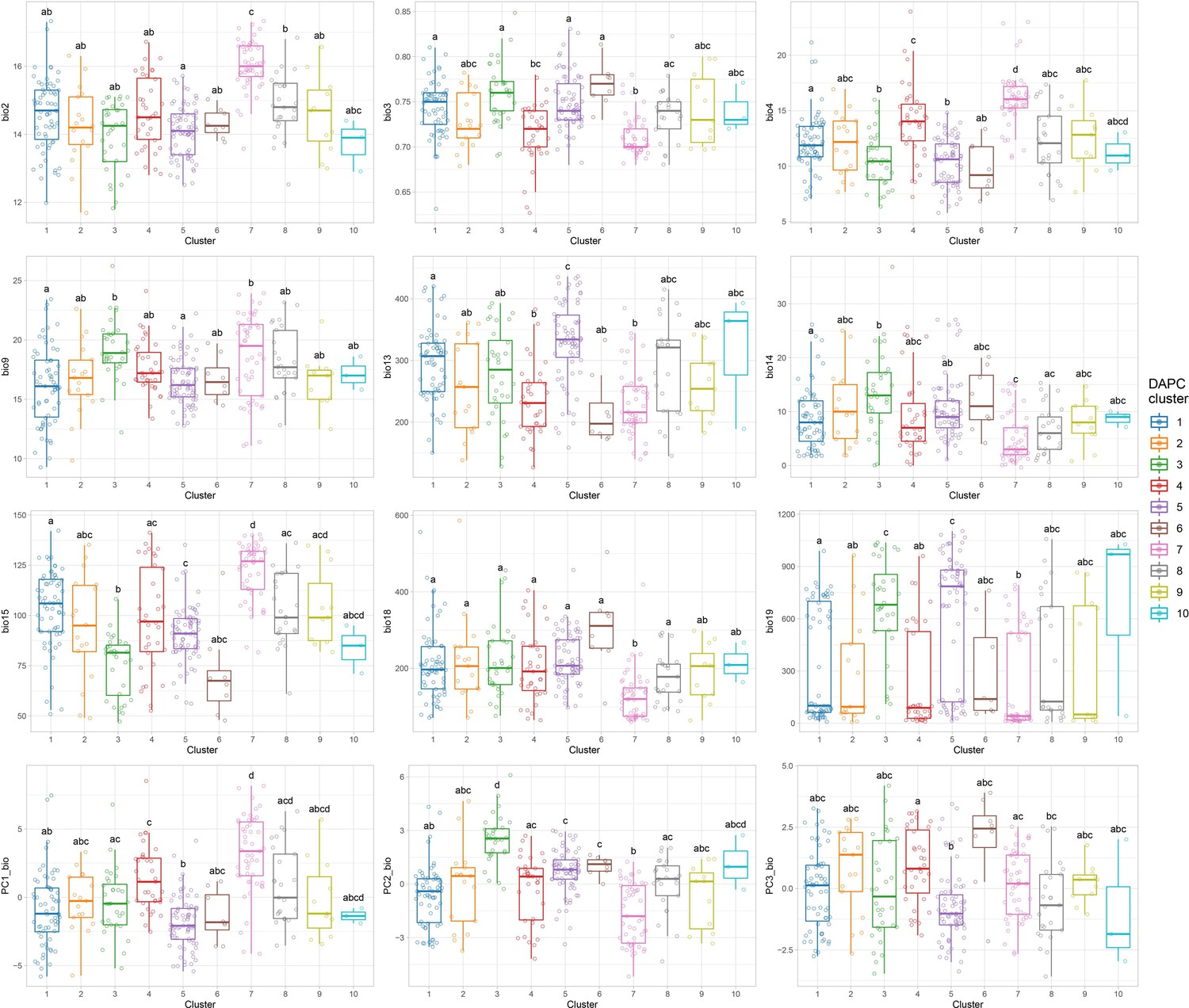
Bioclimatic differences among the 10 discriminant analysis of principal component (DAPC) clusters.
Comparisons among clusters were performed using the pairwise Wilcoxon rank sum test with Bonferroni correction for multiple testing. Letters on top of boxplots denote significance levels, with same letters indicating nonsignificant differences. Only non-collinear bioclimatic variables are shown. Bio2: mean diurnal temperature range; Bio3: Iisothermality; Bio4: Ttemp. Seasonality; Bio9: Mean Temp. of Driest Quarter; Bio13: Precipitation of Wettest Month; Bio14: Precipitation of Driest Month; Bio15: Precipitation Seasonality; Bio18: Precipitation of Warmest Quarter; Bio19: Precipitation of Coldest Quarter. PC1_bio: first bioclimatic principal component; PC2_bio: second bioclimatic principal component; PC3_bio: third bioclimatic principal component.
Figure 2—figure supplement 2
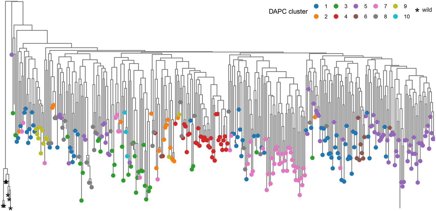
Neighbor-joining phylogenetic trees of the Ethiopian Teff Diversity Panel (EtDP) rooted with wild relative accessions Eragrostis pilosa and Eragrostis curvula.
Tree tips are colored based on the discriminant analysis of principal component (DAPC) genetic clusters. Wild relatives are reported to the left of the tree, marked with star signs.
Figure 3 with 2 supplements
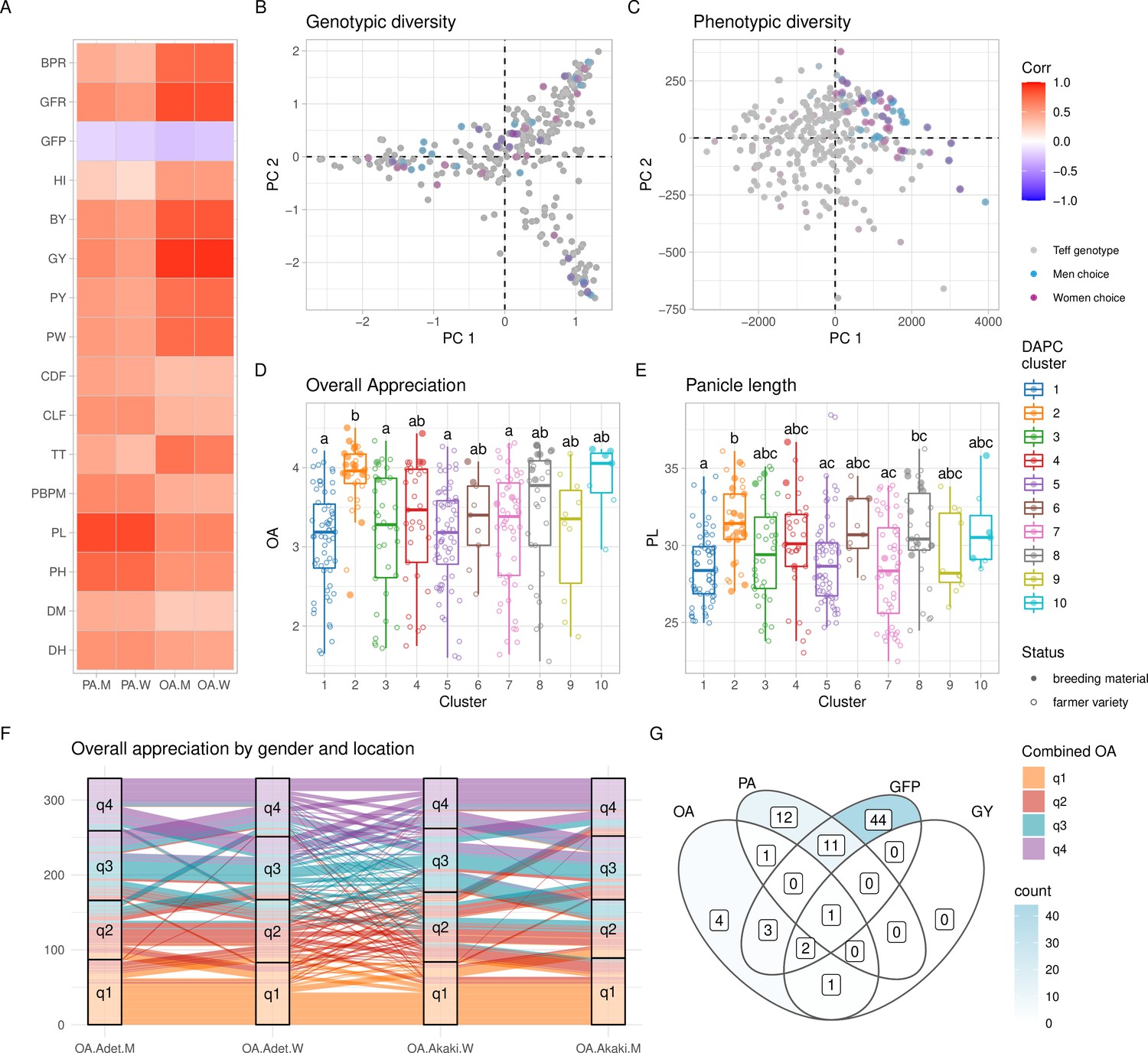
Phenotypic diversity in the Ethiopian Teff Diversity Panel (EtDP).
(A) Pearson’s correlations between agronomic traits (y-axis) and farmer preference traits, by gender (x-axis). Correlation values are expressed in color shades, as indicated in the the legend. (B, C) Top ranking genotypes (90th percentile of the OA distribution) selected by men (blue) and women (purple) farmers, overlaid to the principal component analysis (PCA) of the EtDP genetic diversity (B) and phenotypic diversity (C). Genotypes that were not selected are reported as gray dots. When men and women select the same genotype, the corresponding point appears in dark violet. Trait distribution across discriminant analysis of principal component (DAPC) clusters, for overall appreciation (D) and panicle length (E). Farmer varieties are represented by open circles, improved lines are represented by full circles. (F) Alluvial plot reporting the consistency of farmers’ choice by quartiles of the OA distribution. Each vertical bar represents a combination of location (Adet, Akaki) and gender (M, W). EtDP accessions are ordered on the y-axis according to their OA score in each combination. Alluvial flows are colored according to OA quartiles combined across gender and across location according to the legend (q1, q2, q3, and q4). (G) Venn diagram reporting farmer varieties having values superior to the 75th percentile of the trait distribution of improved varieties (lower than the 25th percentile in the case of GFP). Each area of the Venn diagram reports the corresponding number of farmer varieties, as in the legend. DH, days to heading; DM, days to maturity; PH, plant height; PL, panicle length; PBPM, number of primary branches per main shoot panicle; TT, total tillers; CLF, first culm length; CDF, first culm diameter; PW, panicle weight; PY, panicle yield; GY, grain yield; BY, biomass yield; HI, harvest index; GFP, grain filling period; GFR, grain filling rate; BPR, biomass production rate; OA, overall appreciation; PA, panicle appreciation. This figure has two figure supplements.
Figure 3—figure supplement 1

Correlations between agronomic traits and participatory varietal selection (PVS) traits, by location and gender.
PVS traits are grouped to the top and right of the plot. The pairwise matrix in the plot represents correlation coefficients, as indicated in the legend to the right. When specific by location, the trait code is attached to either Akaki or Adet. When specific by gender, M (men) or W (women) is attached. DH, days to heading; DM, days to maturity; PH, plant height; PL, panicle length; PBPM, number of primary branches per main shoot panicle; TT, total tillers; CLF, first culm length; CDF, first culm diameter; PW, panicle weight; PY, panicle yield; GY, grain yield; BY, biomass yield; HI, harvest index; GFP, grain filling period; GFR, grain filling rate; BPR, biomass production rate; OA, overall appreciation; PA, panicle appreciation.
Figure 3—figure supplement 2
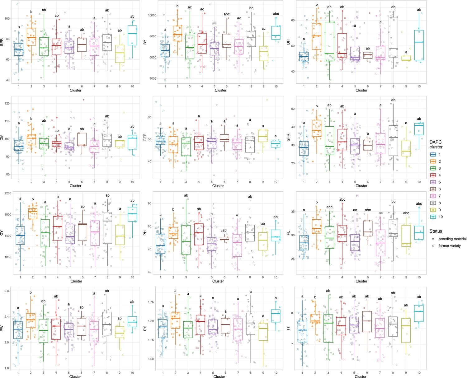
Phenotypic differences among the 10 discriminant analysis of principal component (DAPC) clusters.
Comparisons among clusters were performed using the pairwise Wilcoxon rank sum test with Bonferroni correction for multiple testing. Letters on top of boxplots denote significance levels, with same letters indicating nonsignificant differences. Only traits with significant differences are shown. DH, days to heading; DM, days to maturity; PH, plant height; PL, panicle length; PBPM, number of primary branches per main shoot panicle; TT, total tillers; CLF, first culm length; CDF, first culm diameter; PW, panicle weight; PY, panicle yield; GY, grain yield; BY, biomass yield; HI, harvest index; GFP, grain filling period; GFR, grain filling rate; BPR, biomass production rate; OA, overall appreciation; PA, panicle appreciation.
Figure 4 with 7 supplements
Teff genomic offset.
(A) Geographic distribution of climate-driven allelic variation under current climates across the teff cropping area, with colors representing the three principal component (PC) dimensions reported in panel (B). (C) Genomic vulnerability across the teff cropping area based on the RCP8.5 climate projections. The color scale indicates the magnitude of the mismatch between current and projected climate-driven turnover in allele frequencies according to legend. Phenotyping locations are shown with yellow diamonds. This figure has seven figure supplements.
Figure 4—figure supplement 1
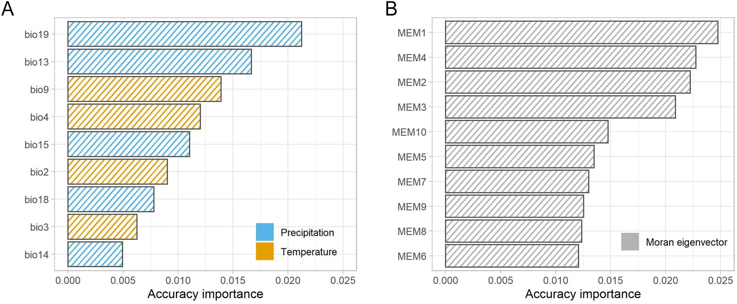
Ranked accuracy and importance of bioclimatic (A) and geographic (Moran’s eigenvector map [MEM]).
(B) Variables in predicting turnover in allele frequency using gradient forest analysis. Genomic composition is best predicted by MEMs one to four and precipitation variables (bio19 and bio13).
Figure 4—figure supplement 2
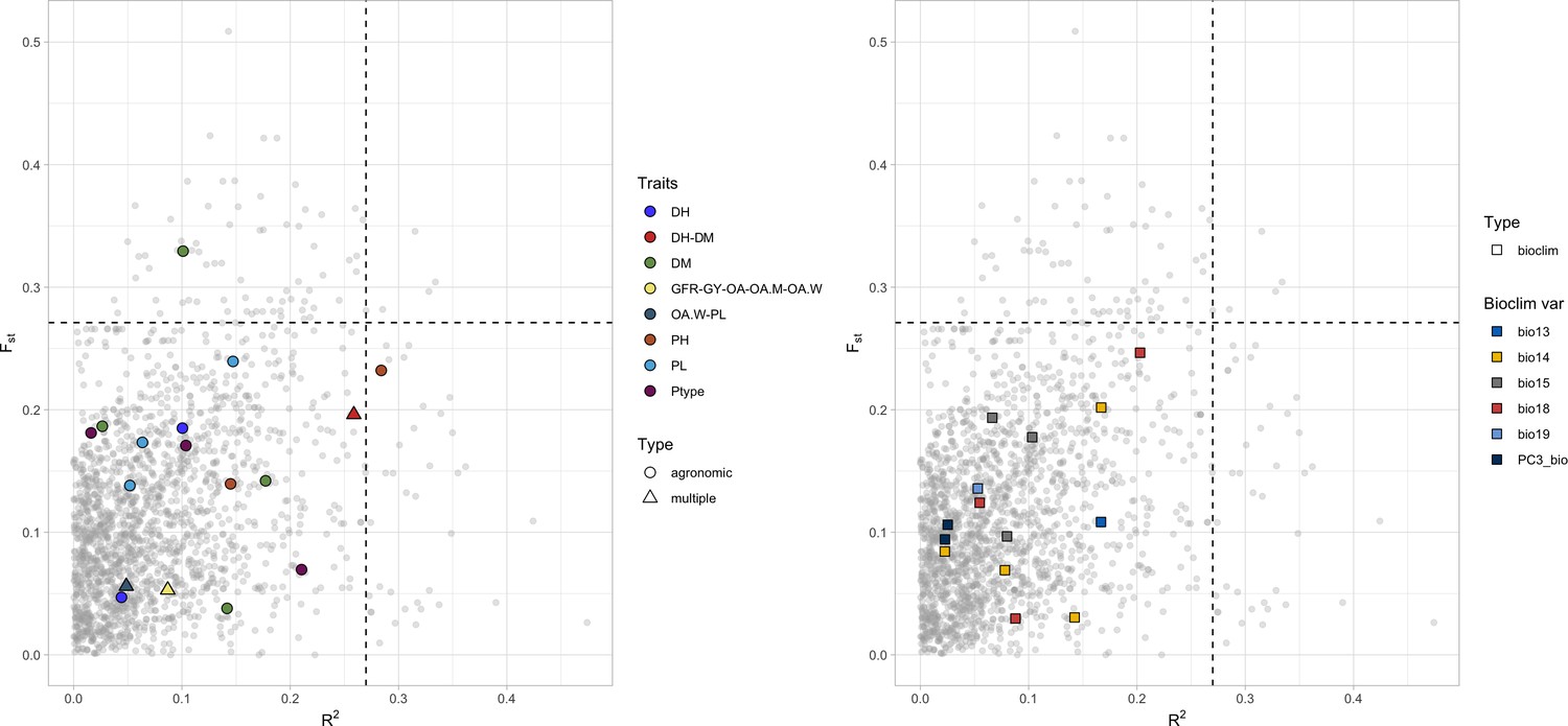
Linkage disequilibrium (LD) blocks distribution in relation to Fst (y-axis) and GF r2 values (x-axis).
LD blocks with null r2 values toward the GF are not shown. LD blocks containing quantitative trait nucleotides (QTNs) are highlighted with colors according to legend. The left-side panel shows agronomic and farmer traits, while the right-side panel QTNs of bioclimatic traits. In both panels, shapes denote whether QTN target a single trait or rather multiple traits. DH, days to heading; DM, days to maturity; PH, plant height; PL, panicle length; GY, grain yield; GFR, grain filling rate; Ptype, panicle type; PA, panicle appreciation; OA, overall appreciation; OA.W, overall appreciation women; OA.M, overall appreciation men.
Figure 4—figure supplement 3
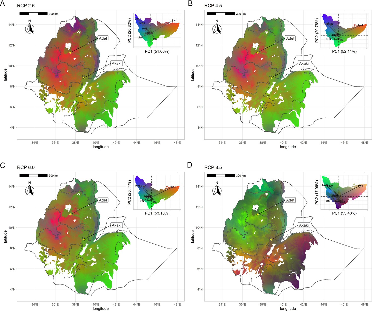
Geographic distribution of climate-driven allelic variation under four representative concentration pathways: (A) RCP2.6, (B) RCP4.5, (C) RCP6.0, and (D) RCP8.5.
Colors are based on principal components analysis (PCA) of transformed climate variables where red is defined by values of PC1 + PC2, green by negative values of PC2, and blue by PC3 + PC2 − PC1 (as in the reference manual). Similar colors in the maps represent similar allele frequencies at climate-responsive loci.
Figure 4—figure supplement 4
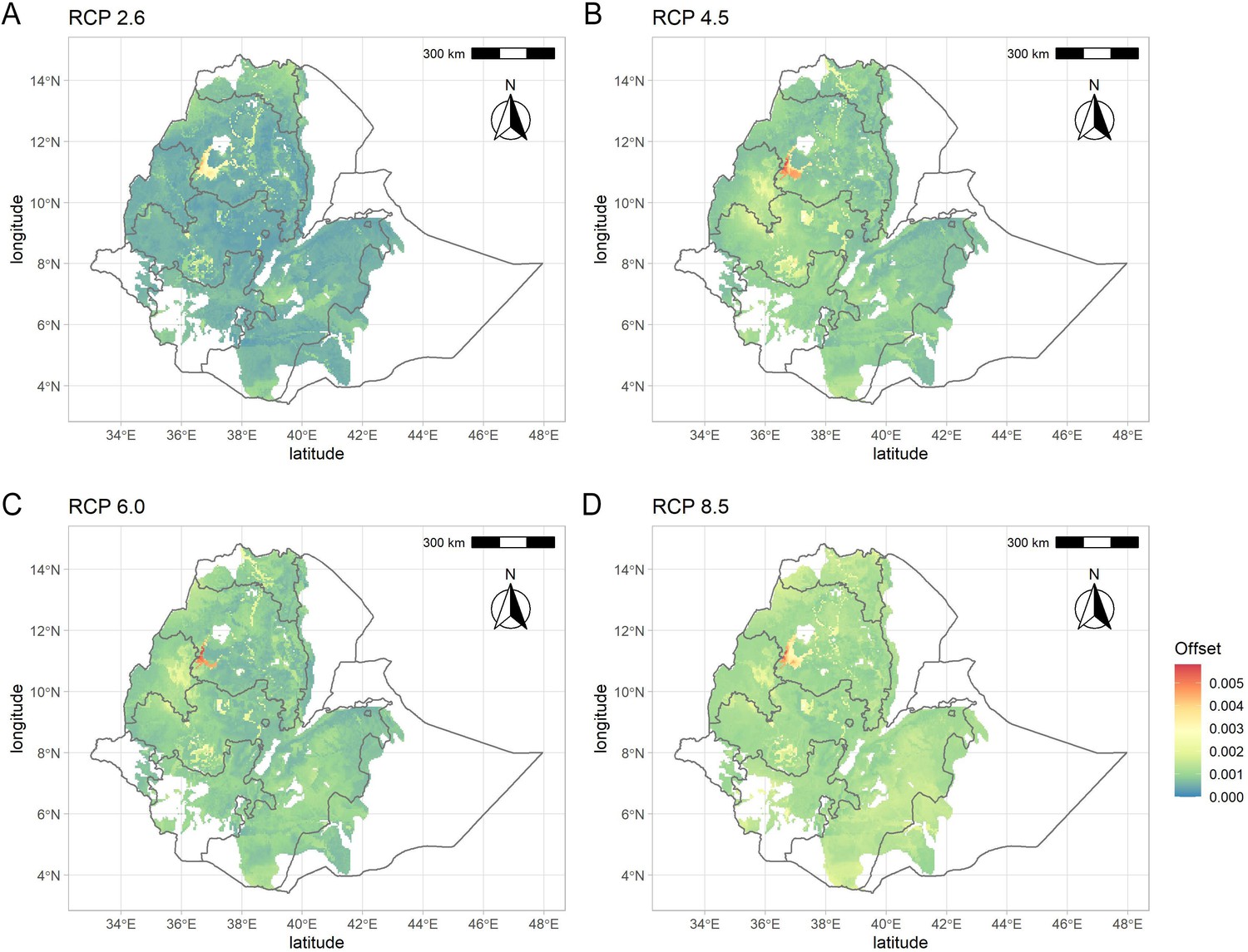
Genomic vulnerabilities in the teff cropping area based on projections for four representative concentration pathways: (A) RCP2.6, (B) RCP4.5, (C) RCP6.0, and (D) RCP8.5.
The color scale indicates the magnitude of the mismatch (i.e., Euclidean distance) between current and projected climate-driven turnover in allele frequencies.
Figure 4—figure supplement 5
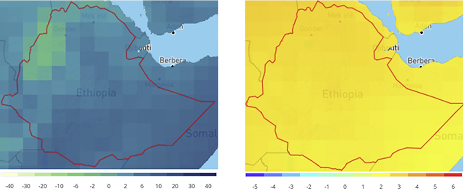
Projected change in Ethiopian climate for 2070s under RCP8.5 compared to 1986–2005.
The plots show the ensemble monthly mean change over 12 months in precipitation (mm) (left) and temperature (°C) (right).
Figure 4—figure supplement 6
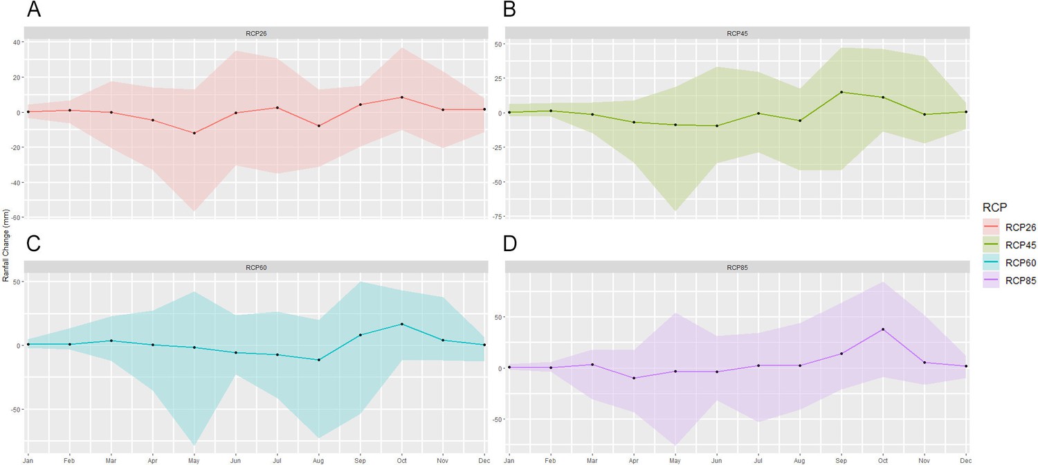
Mean change in monthly rainfall compared to the reference period in the south Lake Tana (36.5–37.75 east,10.7–12 north) by 2070 under RCP2.6 (low emissions), RCP4.5 (medium-low emission), RCP6.0 (medium-high emission), and RCP8.5 (high emission) scenarios.
The shaded region shows the ensemble members' 10–90th percentile ranges.
Figure 4—figure supplement 7
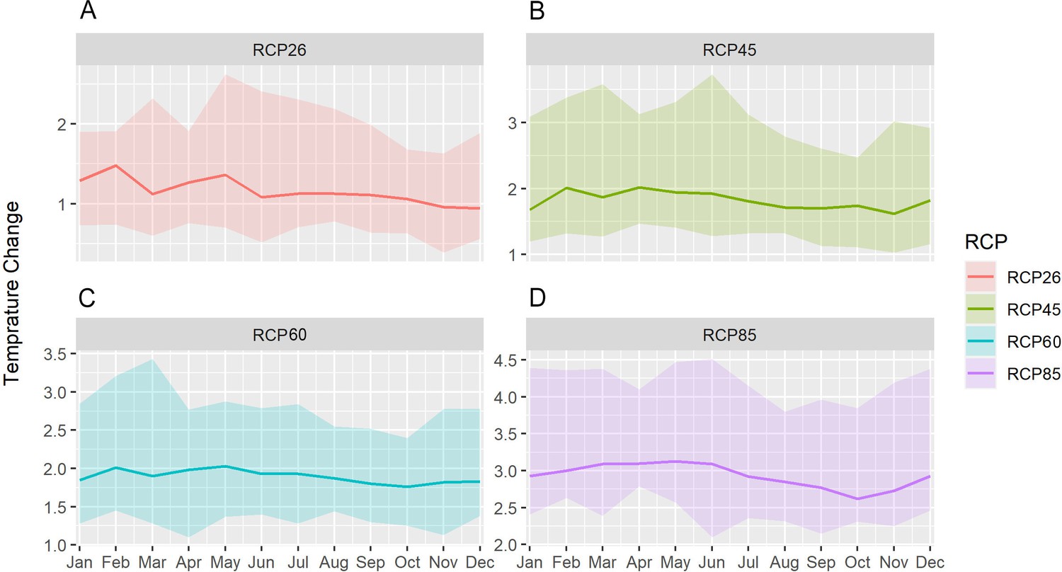
Mean change in monthly temperature compared to the reference period in the south Lake Tana (36.5–37.75 east, 10.7–12 north) by 2070 under RCP2.6 (low emissions), RCP4.5 (medium-low emission), RCP6.0 (medium-high emission), and RCP8.5 (high emission) scenarios.
The shaded region shows the ensemble members' 10–90th percentile ranges.
Figure 5 with 2 supplements
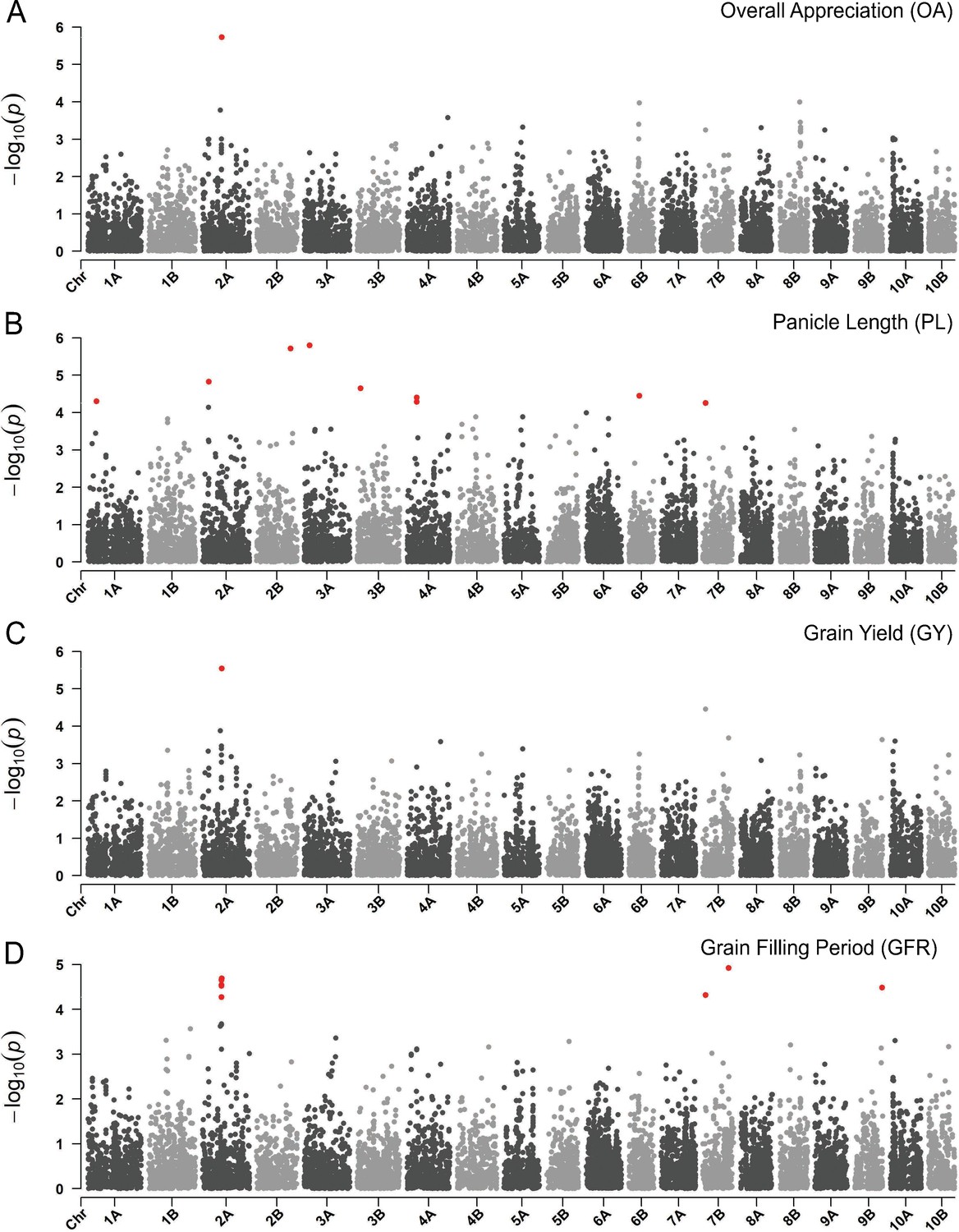
Manhattan plots reporting the genome-wide association study (GWAS) result for.
(A) Overall appreciation, (B), panicle length, (C) grain yield, and (D) grain filling period. On the x-axis, the genomic position of markers. The y-axis reports the strength of the association signal. Single-nucleotide polymorphisms (SNPs) are ordered by physical position and grouped by chromosome. Quantitative trait nucleotides (QTNs), for example SNPs surpassing a threshold based on a false discovery rate of 0.05, are highlighted in red. A strong signal on chromosome 2A matches across participatory varietal selection (PVS) and metric traits. This figure has two supplements.
Figure 5—figure supplement 1
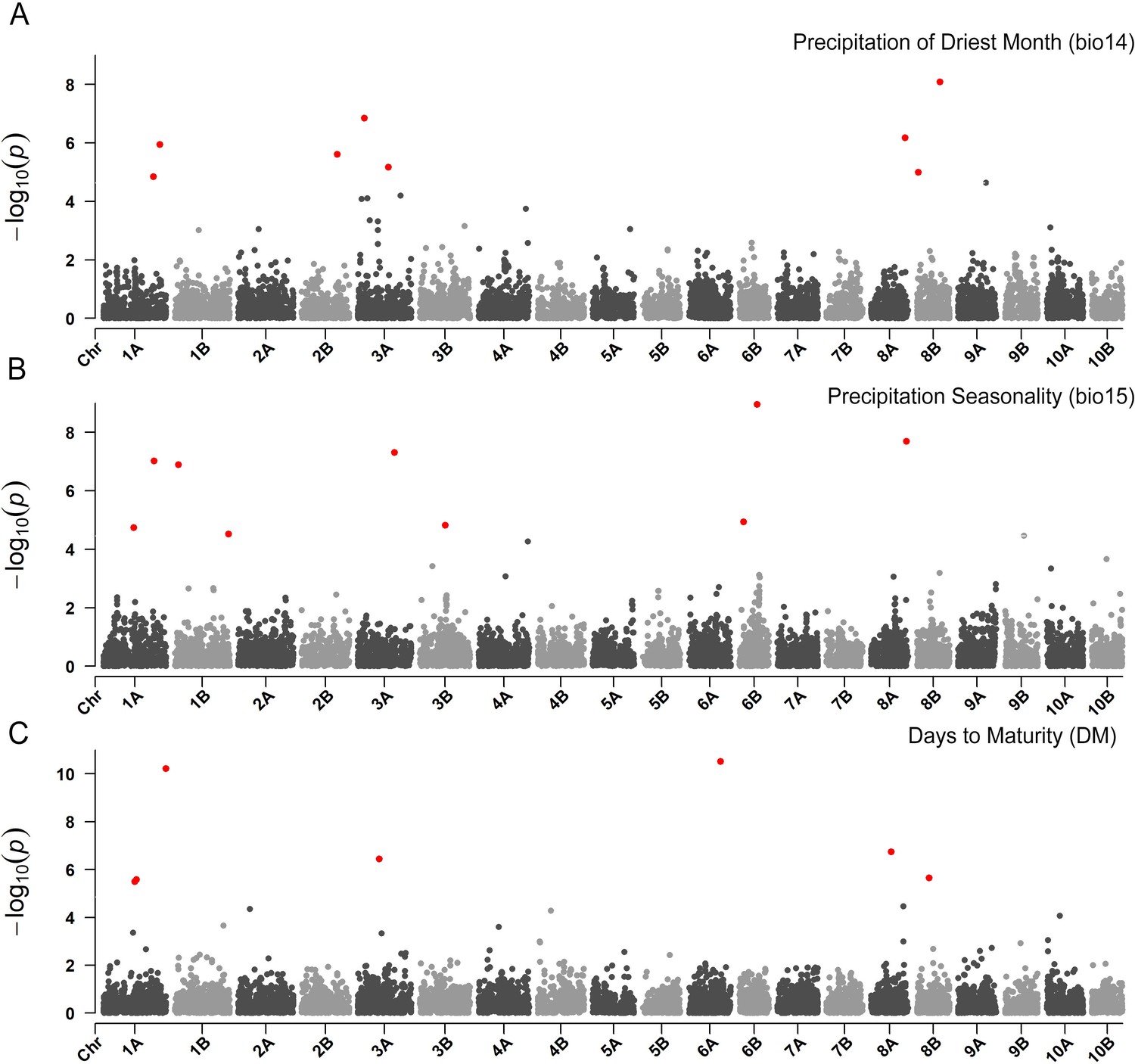
Manhattan plots reporting the genome-wide association study (GWAS) result for (A) precipitation of the driest month, (B) precipitation seasonality and (C) days to maturity. On the x-axis, the genomic position of markers.
The y-axis reports the strength of the association signal. Single-nucleotide polymorphisms (SNPs) are ordered by physical position and grouped by chromosome. Quantitative trait nucleotides (QTNs), for example SNPs surpassing a threshold based on a false discovery rate of 0.05, are highlighted in red.
Figure 5—figure supplement 2
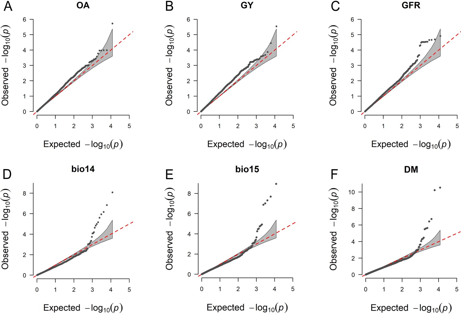
Quantile–quantile plots for the genome-wide association study (GWAS) scans reported in Figure 5A, C and D.
On the x-axis, the expected distribution of p values according to the null hypothesis of no association. On the y-axis, the observed distribution of p values. Each point represents an individual statistical test.
Tables
Table 1
Heritabilities (H2) for farmers’ participatory variety selection traits.
H2 values are given for each trait, type, and location combination. PA, panicle appreciation; OA, overall appreciation; M, men; W, women; ALL, measures combined by either type or location.
| Trait | Type | Location | H2 |
|---|---|---|---|
| PA | ALL | ALL | 0.48 |
| PA | ALL | Adet | 0.50 |
| PA | ALL | Akaki | 0.65 |
| PA | M | ALL | 0.43 |
| PA | W | ALL | 0.45 |
| PA | M | Adet | 0.35 |
| PA | W | Adet | 0.40 |
| PA | M | Akaki | 0.25 |
| PA | W | Akaki | 0.34 |
| OA | ALL | ALL | 0.81 |
| OA | ALL | Adet | 0.71 |
| OA | ALL | Akaki | 0.87 |
| OA | M | ALL | 0.74 |
| OA | W | ALL | 0.74 |
| OA | M | Adet | 0.53 |
| OA | W | Adet | 0.66 |
| OA | M | Akaki | 0.88 |
| OA | W | Akaki | 0.62 |
Table 2
Heritabilities (H2) for agronomic traits.
H2 values are given for each trait, and location combination. DH, days to heading; DM, days to maturity; PH, plant height; PL, panicle length; PBPM, number of primary branches per main shoot panicle; TT, total tillers; CLF, first culm length; CDF, first culm diameter; PW, panicle weight; PY, panicle yield; GY, grain yield; BY, biomass yield; HI, harvest index; GFP, grain filling period; GFR, grain filling rate; BPR, biomass production rate; ALL, measures combined by location.
| Trait | Location | H2 |
|---|---|---|
| DH | ALL | 0.99 |
| DH | Adet | 0.96 |
| DH | Akaki | 0.97 |
| DM | ALL | 0.98 |
| DM | Adet | 0.90 |
| DM | Akaki | 0.89 |
| PH | ALL | 0.16 |
| PH | Adet | 0.92 |
| PH | Akaki | 0.90 |
| PL | ALL | 0.37 |
| PL | Adet | 0.88 |
| PL | Akaki | 0.81 |
| PBPM | ALL | 0.64 |
| PBPM | Adet | 0.83 |
| PBPM | Akaki | 0.83 |
| TT | ALL | 0.25 |
| TT | Adet | 0.65 |
| TT | Akaki | 0.60 |
| CLF | ALL | 0.13 |
| CLF | Adet | 0.88 |
| CLF | Akaki | 0.85 |
| CDF | ALL | 0.15 |
| CDF | Adet | 0.95 |
| CDF | Akaki | 0.96 |
| PW | ALL | 0.27 |
| PW | Adet | 0.90 |
| PW | Akaki | 0.88 |
| PY | ALL | 0.25 |
| PY | Adet | 0.92 |
| PY | Akaki | 0.91 |
| GY | ALL | 0.42 |
| GY | Adet | 0.92 |
| GY | Akaki | 0.93 |
| BY | ALL | 0.34 |
| BY | Adet | 0.84 |
| BY | Akaki | 0.80 |
| HI | ALL | 0.78 |
| HI | Adet | 0.68 |
| HI | Akaki | 0.76 |
| GFP | ALL | 0.96 |
| GFP | Adet | 0.79 |
| GFP | Akaki | 0.83 |
| GFR | ALL | 0.52 |
| GFR | Adet | 0.90 |
| GFR | Akaki | 0.92 |
| BPR | ALL | 0.32 |
| BPR | Adet | 0.80 |
| BPR | Akaki | 0.77 |
Table 3
Plackett–Luce estimates from farmer’s overall appreciation (OA) of genotypes associated with genotypes’ agronomic metrics, DM, days to maturity; PH, plant height; PW, panicle weight; GY, grain yield; BY, biomass yield; GFP, grain filling period.
The rankings were analyzed for the whole group (All) and in subsets among gender to assess differences in traits linkages within men and women farmers. * 0.05 < p < 0.01, ** 0.01 < p < 0.001, *** p < 0.001.
| Group | Estimate | Std. error | z value | Pr(>|z|) | ||
|---|---|---|---|---|---|---|
| All | (Intercept) | −7.09 | – | – | – | |
| GY | 0.000764 | 0.000135 | 5.66 | 1.51E−08 | *** | |
| DM | 0.00625 | 0.00402 | 1.56 | 0.12 | ||
| PH | −0.0123 | 0.00275 | −4.46 | 8.17E−06 | *** | |
| PW | −0.0557 | 0.0716 | −0.777 | 0.437 | ||
| BY | −3.6E−05 | 2.72E−05 | −1.32 | 0.186 | ||
| GFP | 0.011 | 0.00484 | 2.27 | 0.0233 | * | |
| Men | (Intercept) | −7.04 | – | – | – | |
| GY | 0.000765 | 0.000175 | 4.36 | 1.29E−05 | *** | |
| DM | 0.00542 | 0.00531 | 1.02 | 0.308 | ||
| PH | −0.0114 | 0.00361 | −3.17 | 0.00155 | ** | |
| PW | −0.0818 | 0.0932 | −0.878 | 0.38 | ||
| BY | −2E−05 | 0.000036 | −0.562 | 0.574 | ||
| GFP | 0.00919 | 0.00637 | 1.44 | 0.149 | ||
| Women | (Intercept) | 15.6 | – | – | – | |
| GY | −0.00084 | 0.00028 | −3.01 | 0.00262 | ** | |
| DM | −0.186 | 0.0101 | −18.5 | <2e−16 | *** | |
| PH | −0.139 | 0.00661 | −20.9 | <2e−16 | *** | |
| PW | 4.4 | 0.195 | 22.6 | <2e−16 | *** | |
| BY | 0.000346 | 5.43E−05 | 6.38 | 1.74E−10 | *** | |
| GFP | −0.136 | 0.0104 | −13.1 | <2e−16 | *** |
Additional files
-
Supplementary file 1
The file contains supplementary tables arranged in separate sheets, from A to G.
(A) Complete Information for the teff samples used in this study. For each accession, the table reports the name of the accession at the germplasm repository (Name), the ID used in this study, the species, the type of materials (Status), the pedigree if known, the source of the accession, research center (Center) and release year if available (EBI, Ethiopian Biodiversity Institute; DZARC, Debre Zeit Agricultural Research Center; AARC, Adet Agricultural Research Center; HARC, Holleta Agricultural Research Center; BARC, Bako Agricultural Research Center; MARC, Melkassa Agricultural Research Center; SARC, Sirinka Agricultural Research Center). For accessions deriving from landraces, the table also reports the corresponding agroecological zone and the region name at three levels (Region_1, Region_2, and Region_3), the longitude, and the latitude. The table then reports the genetic cluster assigned by the analyses, the altitude, and the historical bioclim variables. Finally, BLUP values for phenotypes are farmer traits are reported. When specific by location, the trait code is attached to either Akaki or Adet. When specific by gender, M (men) or W (women) is attached. DH, days to heading; DM, days to maturity; PH, plant height; PL, panicle length; PBPM, number of primary branches per main shoot panicle; TT, total tillers; CLF, first culm length; CDF, first culm diameter; PW, panicle weight; PY, panicle yield; GY, grain yield; BY, biomass yield; HI, harvest index; GFP, grain filling period; GFR, grain filling rate; BPR, biomass production rate; OA, overall appreciation; PA, panicle appreciation. (B) Haplotype blocks for SNPs used in this study. For each SNP, the table reports the SNP name, the chromosome, and the position. If any, the table reports the corresponding haplotype block with start and stop position and number of SNPs in the block. (C) Variance components from BLUP model calculation on agronomic traits and farmer traits. The table reports solution, standard error, z ratio, and percent variance explained for each component of the model for each trait. Trait codes as in Supplemenary File 1A. Factor codes as follows: ID, genotype; REP, replication within the field; LOCATION, field location; F_TYPE, gender; interactions between factors are indicated as in F_TYPE:LOCATION, for example gender by location. (D) Main effects of and interactions between location, genetic cluster, and, in the case of PVS traits, gender, regarding teff traits. Phentoype codes as in (A). Values in the table are p values for a two- (metric traits) and three-way ANOVA (PVS traits). Significant effects are highlighted in bold. (E) Genome-wide association results. For each SNP-trait combination, the table reports the trait name, the SNP name, its chromosome, and position. The reference (REF) and alternative (ALT) allele are reported for each SNP. For each association, the table reports the effect, the standard error (SE), the corresponding p value (pvalue), and multiple-test correction with a q value (qvalue). The number of PC covariates used in the GWAS scan is reported in column n_PC. DH, days to heading; DM, days to maturity; PH, plant height; PL, panicle length; PBPM, number of primary branches per main shoot panicle; TT, total tillers; CLF, first culm length; CDF, first culm diameter; PW, panicle weight; PY, panicle yield; GY, grain yield; BY, biomass yield; HI, harvest index; GFP, grain filling period; GFR, grain filling rate; BPR, biomass production rate; OA, overall appreciation; PA, panicle appreciation. Bio2: mean diurnal temperature range; Bio3: Isothermality; Bio4: Temp. Seasonality; Bio9: Mean Temp. of Driest Quarter; Bio13: Precipitation of Wettest Month; Bio14: Precipitation of Driest Month; Bio15: Precipitation Seasonality; Bio18: Precipitation of Warmest Quarter; Bio19: Precipitation of Coldest Quarter. PC1_bio: first bioclimatic principal component; PC2_bio: second bioclimatic principal component; PC3_bio: third bioclimatic principal component. (F) Candidate genes mining for significant associations. The table reports genes in LD blocks with at least one significant association. Each row reports the Eragrostis tef gene ID (Et_gene), with chromosome, start position, end position, and DNA strand (positive + or negative −). When present, the table reports the closest homolog gene in Arabidopsis (id_At) with the percentual identity in the alignment (perc_identity_At), the E value reported by the BLASTP, the percentual query coverage in the target gene (perc_query_coverage_per_subject_At). The same information is reported for Zea mays (Zm) hits. The table reports the name of the LD block and the number of quantitative trait loci (QTN) in that block. (G) SNPs with adaptation potential. For each marker, the table reports the chromosome, position, Fst values, and gradient forest model fit (GF r2).
- https://cdn.elifesciences.org/articles/80009/elife-80009-supp1-v1.xlsx
-
MDAR checklist
- https://cdn.elifesciences.org/articles/80009/elife-80009-mdarchecklist1-v1.pdf
Download links
A two-part list of links to download the article, or parts of the article, in various formats.
Downloads (link to download the article as PDF)
Open citations (links to open the citations from this article in various online reference manager services)
Cite this article (links to download the citations from this article in formats compatible with various reference manager tools)
Data-driven, participatory characterization of farmer varieties discloses teff breeding potential under current and future climates
eLife 11:e80009.
https://doi.org/10.7554/eLife.80009


