A model of hippocampal replay driven by experience and environmental structure facilitates spatial learning
Figures
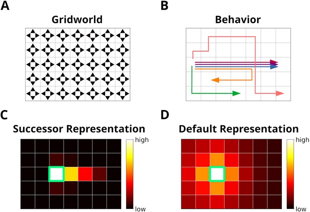
The grid world.
(A) An example of a simple grid world environment. An agent can transition between the different states, that is, squares in the grid, by moving in the four cardinal directions depicted by arrowheads. (B) Example trajectories of an agent moving in the grid world. (C) The successor representation (SR) for one state (green frame). Note that the SR depends on the agent’s actual behavior. (D) The default representation (DR) for the same state as in C. In contrast to the SR, the DR does not depend on the agent’s actual behavior and is equivalent to the SR given random behavior.
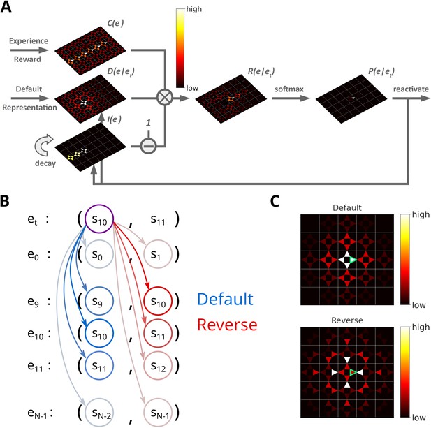
Illustration of the Spatial structure and Frequency-weighted Memory Access (SFMA) replay model.
(A) The interaction between the variables in our replay mechanism. Experience strength , experience similarity and inhibition of return are combined to form reactivation prioritization ratings. Reactivation probabilities are then derived from these ratings. (B) Experience tuples contain two states: the current state and next state. In the default mode, the current state of the currently reactivated experience (violet circle) is compared to the current states of all stored experiences (blue arrows) to compute the experience similarity . In the reverse mode, the current state of the currently reactivated experience is compared to the next state of all stored experiences (red arrows). (C) Example of the similarity of experiences to the currently reactivated experience (green arrow) in an open field for the default and reverse modes. Experience similarity is indicated by the colorbar. In the default mode, the most similar experiences are the current state or those nearby. In the reverse mode, the most similar experiences are those that lead to the current state.
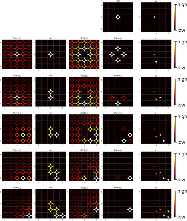
Step by step example of a replay sequence generated by SFMA.
From left to right: the different variables of SFMA as well as the reactivated experiences. Experience strength had the same value for all experiences and was therefore omitted. From top to bottom: the replay steps from start to finish. Replay was initiated at the center of the environment. Note that for replay initialization the prioritization variables do not convey information and were therefore omitted.
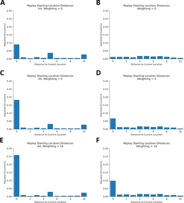
Reconciling non-local replays and preferential replay for current location in online replay.
(A) Histogram of starting locations of offline replay recorded in the virtual version of Gupta et al.’s experiment. Raw occurrences for each bin were divided by the maximum number of bin occurrences to account for uneven distribution of distance bins. Replays were recorded at either of the reward locations. Current locations are over-represented, but replay is also initiated at other locations (non-local replay). (B) Same as in A, but in an open field environment with no reward and homogeneous experience strengths. Replays were recorded at different locations in the environment. Non-local replays are prevalent, but there is no preference for the current location – contrary to observations of online replay. (C/D) Same as A/B, but the experience strengths close to current location were increased to model an initialization bias. In both environments, the current location is more strongly represented by replays and non-local replays occur. (C/D) Same as C/D, but with a stronger increase of experience strengths. The current location is more even more strongly represented by replays.
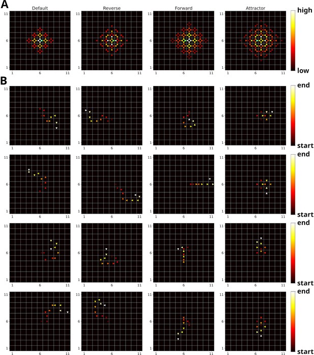
Possible replay modes and example replay trajectories.
(A) Experience similarities of the different replay modes, that is, default, reverse, forward and attractor mode, for a given experience (marked in green). (B) Example replay trajectories generated in an open field environment with the different replay modes (from left to right: default, reverse, forward, and attractor mode). Experience strengths were homogeneous and replay was initiated in the center of the environment.
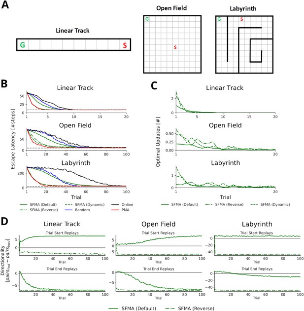
Statistics of replay has large impact on spatial learning.
(A) The three goal-directed navigation tasks that were used to test the effect of replay on learning: linear track, open field and maze. In each trial, the agent starts at a fixed starting location S and has to reach the fixed goal location G. (B) Performance for different agents measured as the escape latency over trials. Shown is the performance for an online agent without replay (black), an agent that was trained with random replay (blue), our SFMA model (green), and the Prioritized Memory Access model (PMA) by Mattar and Daw, 2018 (red). The results of our SFMA model are further subdivided by the replay modes: default (solid), reverse (dash-dotted), and dynamic (dashed). Where the dashed and dash-dotted green lines are not visible they are overlapped by the red solid line. (C) Reverse and dynamic replay modes produce more optimal replays while the default replay mode yields pessimistic replays. Shown is the number of optimal updates in the replays generated on each trial for different replay modes: default (solid), reverse (dash-dotted), and dynamic (dashed). Note, that in later trials there is a lack of optimal updates because the learned policy is close to the optimal one and any further updates have little utility. (D) Directionality of replay produced by the default (solid) and reverse (dash-dotted) modes in the three environments. The reverse replay mode produces replays with strong reverse directionality irrespective of when replay was initiated. In contrast, the default mode produces replays with a small preference for forward directionality. After sufficient experience with the environment the directionality of replays is predominantly forward for replays initiated at the start and predominantly reverse for replays initiated at the end of a trial.
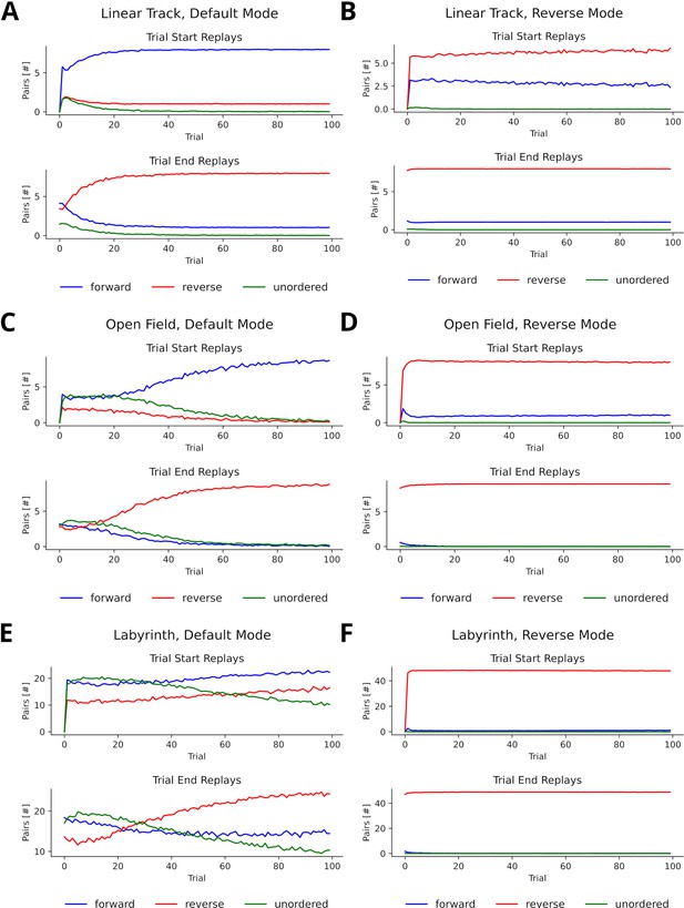
Directionality of consecutive replay pairs.
(A) Pairs produced on a linear track when using the default mode for replays generated at the start (top) and end (bottom) of a trial. A pair of consecutively reactivated experiences and et was considered forward when the next state of was the current state of et, reverse when the current state of was the next state of et and unordered otherwise. (B) Pairs produced on a linear track when using the reverse mode. (C/D) Same as A/B, but in an open field environment. (E/F) Same as A/B, but in a labyrinth environment.
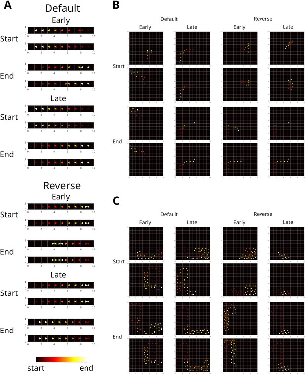
Example replay trajectories in different spatial navigation tasks.
(A) Replay trajectories generated at the start and end of trials in the linear track for different replay modes (default and reverse) and different stages of learning (early and late). Color indicates when in a replay event a transition was replayed. (B) Same as A, but in an open field. (C) Same as A, but in a labyrinth like in Widloski and Foster, 2022.
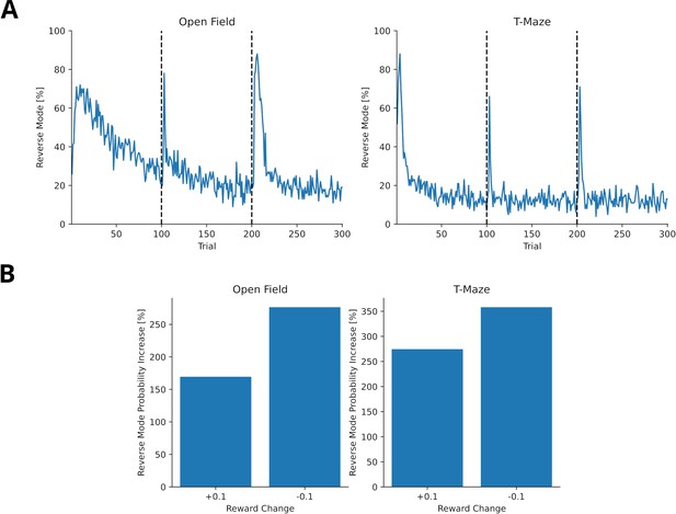
Reward changes trigger higher probability of activating the reverse mode.
(A) The probability of replay being generated in the reverse mode for agents trained in open field (left) and T-maze (right) for 300 trials. Reward was changed once after 100 trials (+0.1) and again after another 100 trials (–0.1). The probability for reverse mode spikes once in the beginning when the reward was first encountered and when the reward changes. (B) The percentage change of reverse mode activation after reward change. Percentage change was computed from the five trial average before and after the reward change.

The number of sequences decreases with experience.
The number of sequences per replay as a function of experienced trials for three different environments, that is, linear track, open field and labyrinth. The replay lengths were 10, 10 and 50, respectively. Early during learning replay contains multiple short sequences. By the end of learning replay tends to represent one long sequence in linear track and open field environments. For the labyrinth environment, the number of sequences is still decreasing due to the complexity of the environment and the much higher replay length.
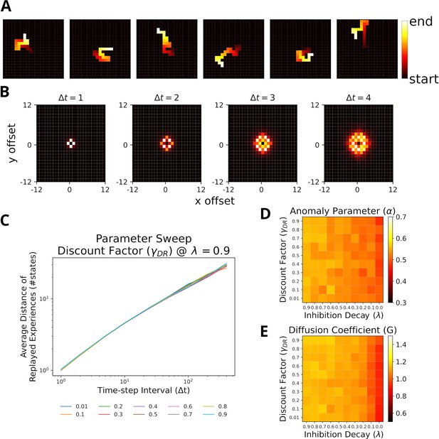
Replays resemble random walks across different parameter values for Default Representation (DR) discount factor and inhibition decay.
(A) Example replay sequences produced by our model. Reactivated locations are colored according to recency. (B) Displacement distributions for four time steps (generated with ). (C) A linear relationship in the log-log plot between average distance of replayed experiences and time-step interval indicates a power-law. Lines correspond to different values of the DR’s discount factor as indicated by the legend. (D) The anomaly parameters (exponent of power law) for different parameter values of DR and inhibition decay. Faster decay of inhibition, which allows replay to return to the same location more quickly, yields anomaly parameters that more closely resemble a Brownian diffusion process, that is, closer to 0.5. (E) The diffusion coefficients for different parameter values of DR and inhibition decay. Slower decay of inhibition yields higher diffusion coefficients.
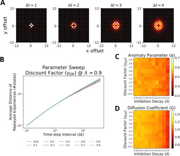
Replays generated using the reverse mode also resemble random walks across different parameter values.
Replays generated using the reverse mode also resemble random walks across different parameter values for Default Representation (DR) discount factor and inhibition decay. (A) Displacement distribution for the first four time steps. (B) Our model can reproduce the linear log-log relationship between time-step interval and average distance of replayed experiences. (C) The anomaly parameters for different parameter values of DR and inhibition decay. Faster decay of inhibition yields anomaly parameters which closer resemble a Brownian diffusion process (i.e. closer to 0.5). (D) The diffusion coefficients for different parameter values of DR and inhibition decay. Slower decay of inhibition yields higher diffusion coefficients.
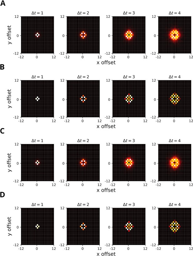
Displacement distributions for different inverse temperature values.
Displacement distributions for different inverse temperature values ( and ). (A) Displacement distribution for the first four time steps with given homogeneous experience strength. (B) The same as A, but with a higher inverse temperature. Note the lower local variance of the distribution compared to A. (C) The same as A, but given heterogeneous experience strengths. (D) The same as C, but with. Note the negligible difference between homogeneous and heterogeneous experience strengths.
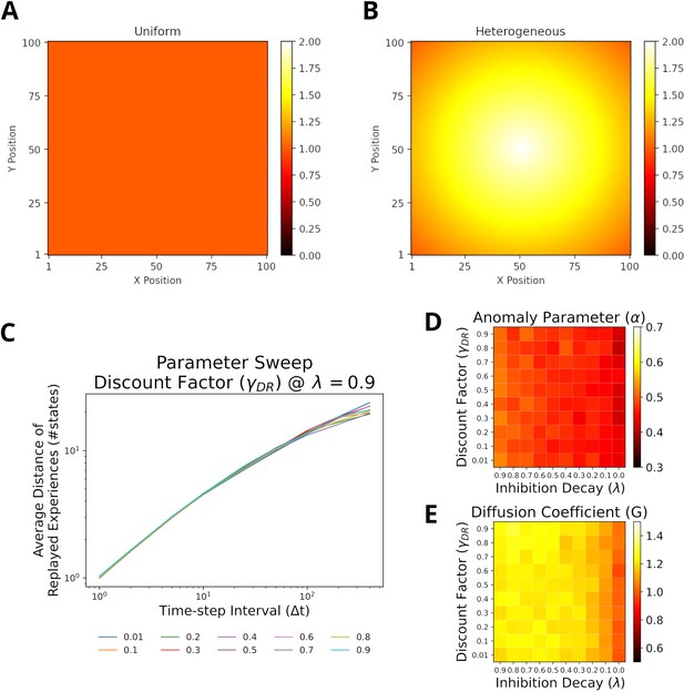
For heterogeneous experience strengths replays also resemble random walks across different parameter values.
For heterogeneous experience strengths replays also resemble random walks across different parameter values for Default Representation (DR) discount factor and inhibition decay. (A) Homogeneous experience strength condition. (B) Heterogeneous experience strength condition. (C) Our model can reproduce the linear log-log relationship between time-step interval and average distance of replayed experiences. (D) The anomaly parameters for different parameter values of DR and inhibition decay. Faster decay of inhibition yields anomaly parameters which closer resemble a Brownian diffusion process (i.e., closer to 0.5). (E) The diffusion coefficients for different parameter values of DR and inhibition decay. Slower decay of inhibition yields higher diffusion coefficients.
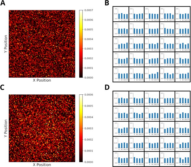
The starting positions of replay are randomly distributed across the environment.
The starting positions of replay are randomly distributed across the environment in a 2-d open field. (A) Distribution of replay starting positions given homogeneous experience strengths. Starting positions are distributed (>90% randomness) evenly across the environment. Randomness of starting locations was measured like in Stella et al., 2019. (B) Initial direction of replays are evenly distributed given homogeneous experience strengths. The environment was divided into bins of size 20x20. (C/D) Same as A/B, but with heterogeneous experience strengths.
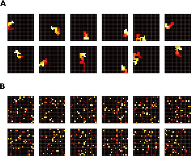
Prioritized Memory Access’ (PMA) ability to produce sequences is severely disrupted when the gain calculation for n-step updates is adjusted.
(A) Sequences generated by PMA (Mattar and Daw, 2018) given uniform need and all-zero gain. Because utility is defined as a product of gain and need, the gain must have a nonzero value to prevent all-zero utility values. This is achieved by applying a (small) minimum gain value. For n-step updates, which update the Q-function for all n steps along the trajectory and are the main driver for forward replay sequences in PMA, the gains are summed across all n steps. Mattar and Daw, 2018 apply the minimum gain value before summation, which artificially increases the gain of n-step updates. (B) Same as A, but the minimum gain value is enforced after summing gain along the steps of the n-step update. We argue that the minimum value should be applied after the summation of gain values, since otherwise the gain artificially increases with sequence length. If done so, PMA loses the ability to produce forward sequences and starts to randomly reactivate experiences.
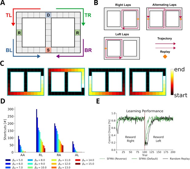
Replay of shortcuts results from stochastic selection of experiences and the difference in relative experience strengths.
(A) Simplified virtual version of the maze used by Gupta et al., 2010. The agent was provided with reward at specific locations on each lap (marked with an R). Trials started at bottom of the center corridor (marked with an S). At the decision point (marked with a D), the agent had to choose to turn left or right in our simulations. (B) Running patterns for the agent used to model different experimental conditions: left laps, right laps and alternating laps. Replays were recorded at the reward locations. (C) Examples of shortcut replays produced by our model. Reactivated locations are colored according to recency. (D) The number of shortcut replays pooled over trials for different running conditions and values of the inverse temperature . Conditions: alternating-alternating (AA), right-left (RL), right-alternating (RA), and alternating-left (AL). (E) Learning performance for different replay modes compared to random replay. The agent’s choice depended on the Q-values at the decision point. The agent was rewarded for turning right during the first 100 trials after which reward shifted to the left (red line marks the shift).
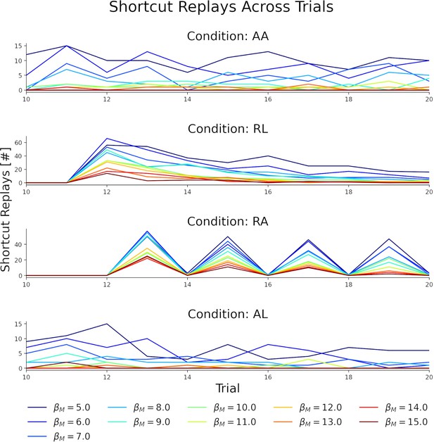
Number of shortcut replays on a trial by trial basis differs depending on behavioral statistics.
Shortcut replays in each trial for different experimental conditions: alternating-alternating (AA), right-left (RL), right-alternating (RA) and alternating-left (AL). For all conditions the number of shortcut replays is affected by the choice of the inverse temperature parameter.
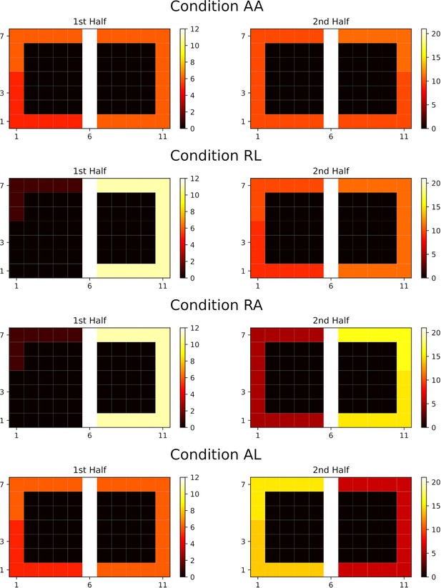
Experience strengths resulting from different behavioral statistics in Gupta et al., 2010 experiment.
Experience strengths after the first (left panels) and second half (right panels) given the different behavioral statistics (rows). For simplicity, the experience strength shown in each state is the sum over the four potential actions. Conditions: alternating-alternating (AA), right-left (RL), right-alternating (RA), and alternating-left (AL).
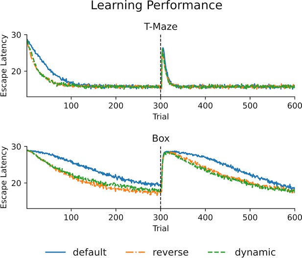
Following strongly stereotypical behavior efficient learning occurs for the default mode after a change in goal location.
Top: he learning performance for different replay modes in a T-maze environment. The goal arm changes after 300 trials. For learning of the initial goal, the default mode is clearly outperformed by reverse and dynamic modes. However, there is no difference in learning performance between the different modes for learning the new goal location. Bottom: Same as for the top panel, but for an open field (Box), which allows for more variability in behavior (i.e. less stereotypical behavior). Learning performance is overall worse for all modes. The default mode is outperformed by the other two modes for both goal locations.
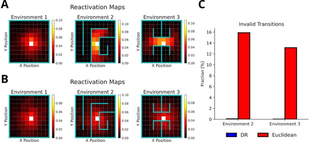
The default representation (DR) allows replay to adapt to environmental changes.
(A) Reactivation maps, that is, the fraction of state reactivations, for all replays recorded in three environments while the agent is located at the white square. Experience similarity is based on the DR with a discount factor . The colorbar indicates the fraction of reactivations. Note that replay obeys the current environmental boundaries. (B) Same as in A, but experience similarity is based on the Euclidean distance between states. Note that replay ignores the boundaries. (C) The fraction of invalid transitions during replay in different environments for the DR (blue) and Euclidean distance (red). While replay can adapt to environmental changes when using the DR, it does not when experience similarity is based on the Euclidean distance.
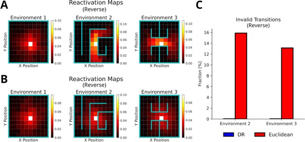
Reverse mode replays adapt to environmental changes.
(A) Reactivation maps, that is, the fraction of state reactivations, for reverse mode replay recorded in three environments (). The color bar indicates the fraction of reactivations across all replays. Note that replay obeys the current environmental boundaries. (B) Same as in A, but experience similarity is based on the Euclidean distance between states. Note that replay ignores the boundaries. (C) The fraction of invalid transitions during reverse model replay in different environments for the DR (blue) and Euclidean distance (red). While replay can adapt to environmental changes when using the DR, it does not when experience similarity is based on the Euclidean distance.
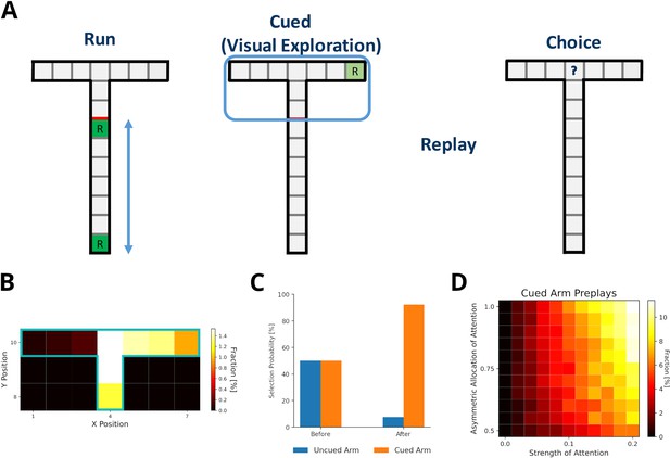
Preplay of cued, but unvisited, locations can be explained by visual exploration.
(A) Schematic of the simplified virtual maze and task design used to model study by Ólafsdóttir et al., 2015. First, in an initial run phase, the agent ran up and down the stem of the maze. Second, in the following visual exploration phase, the agent visually explores a cued part of the maze and increases the strength of the associated experiences. Third, experiences are reactivated according to their priority scores. Fourth, agents are given access to the entire T-maze. The fraction of choosing the two arms in the test phase are compared. (B) Fractions of reactivated arm locations. Experiences associated with the cued arm (right) are preferentially reactivated. (C) The fractions of choosing either arm before and after training the agent with preplay. Before preplay the agent shows no preference for one arm over the other. After preplay, the agent preferentially selects the cued arm over the uncued arm. (D) The percentage of cued-arm preplay (out of all arm preplays and stem replays) for different amounts of attention paid to the cued arm vs. the uncued arm (asymmetric allocation of attention) and experience strength increase relative to actual exploration (attention strength).

Preplay of yet unvisited cued locations can be explained by visual exploration (reverse mode).
(A) Fractions of reactivated arm locations. Experiences associated with the cued arm (right) are preferentially reactivated. (B) The fractions of choosing the cued arm and uncued arm before and after training the agent with preplay. The agent preferentially selects the cued arm after preplay. (C) The percentage of cued-arm preplay for different amounts of attention paid to the cued arm vs. the uncued arm.
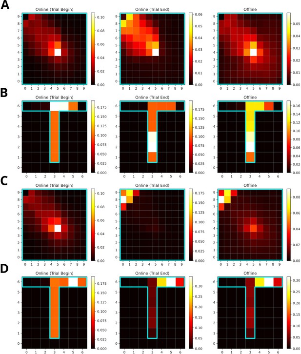
Increasing the reward modulation of experience strengths leads to an over-representation of rewarded locations in replays.
(A) Reactivation maps for online replays generated in an open field environment at trial begin (left) and end (middle) as well as for offline replays (right). Reward modulation was one. Replay tends to over-represent the path leading to the reward location. The starting location is strongly over-represented for all replay conditions, while the the reward location is mainly over-represented for trial end replays. (B) Same as A, but in a T-maze. (C) Same as A, but due to a higher reward modulation of ten the rewarded location is strongly over-represented in replay. (D) Same as C, but in a T-maze.
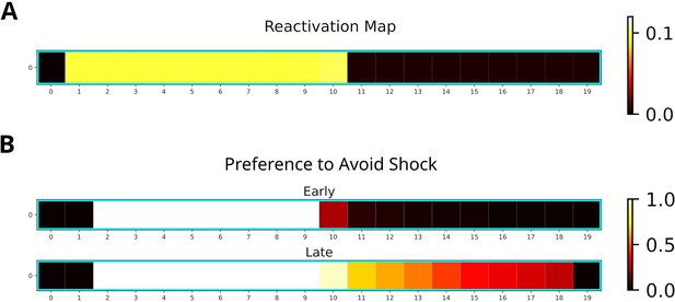
Replay will enter aversive zones given previous experience.
(A) The reactivation map indicates that the dark zone (left half), which contains the shock zone, was preferentially replayed even after the shock administered and the agent stopped in the middle. (B) Probability of the Q-function pointing away from the shock zone for each state. After the first five trials (Early), avoidance is apparent only for states in the dark zone (excluding the shock zone itself). In the following five trials (Late), the preference for avoidance is propagated to the light zone (right half).
Tables
Training settings for each task.
| Environment | Trials | Steps per Trial | Replay Length |
|---|---|---|---|
| Linear Track | 20 | 100 | 10 |
| Open Field | 100 | 100 | 10 |
| Labyrinth | 100 | 300 | 50 |


