Figures and data in Optimal cancer evasion in a dynamic immune microenvironment generates diverse post-escape tumor antigenicity profiles | eLife

Figures
Additional files

5 figures and 1 additional file

Figures

Figure 1 with 11 supplements

Download asset Open asset

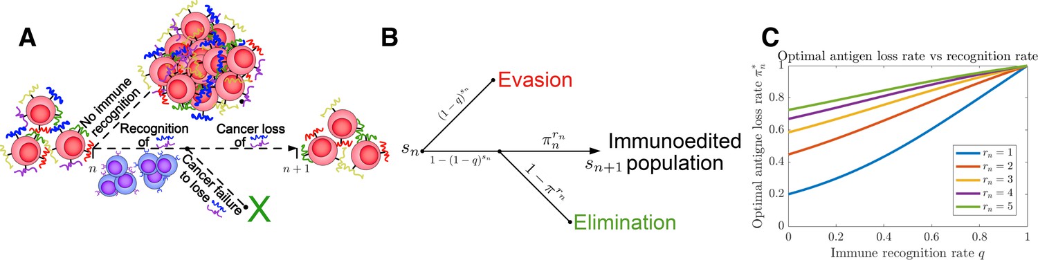
Tumor Evasion via adaptive Antigen Loss (TEAL) model.

(A) Illustration of tumor antigen detection and downregulation in the TEAL model of cancer-immune interaction. (B) The directed graph with nodes representing the states of the TEAL model and edges labeled based on the probability of their occurrence. The interaction leads to elimination, equilibrium, or escape. Both evasion and elimination are absorbing states, and the equilibrium state results in repeated interaction. (C) Plots of single-period cancer optimal antigen loss rates $π^{*}$ given by Equation 8 are plotted as a function of recognition rate $q$ for various numbers of recognized antigens $0 < r_{n} \leq s_{n}$ with $s_{n} = 5$ .

Figure 1—figure supplement 1

Download asset Open asset

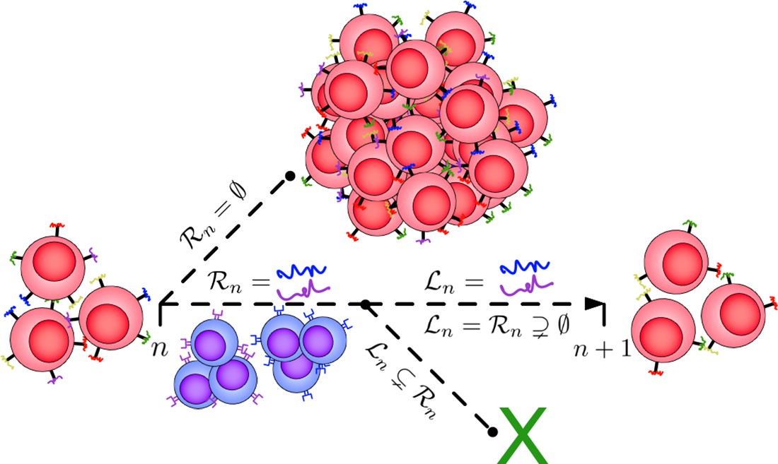
Illustration of the Tumor Evasion via adaptive Antigen Loss (TEAL) model.

A population of cancer cells (red) possesses an initial minimal collection of surface antigens that may be identified and targeted by the immune system (colored antigens). If the immune system is unable to recognize any of these antigens ( $R_{n} = \emptyset$ ), then the cancer grows unchecked to escape size and the process ends. Alternatively, if the immune system (blue cells) recognizes a subset of detectable antigens ( $R_{n} \neq \emptyset$ ), then the cancer population must evolve by generating a clone that has avoided detection through the targeted antigen ( $L_{n} = R_{n}$ ). If this occurs, then the cancer population survives to the next period, otherwise the population becomes extinct.

Figure 1—figure supplement 2

Download asset Open asset

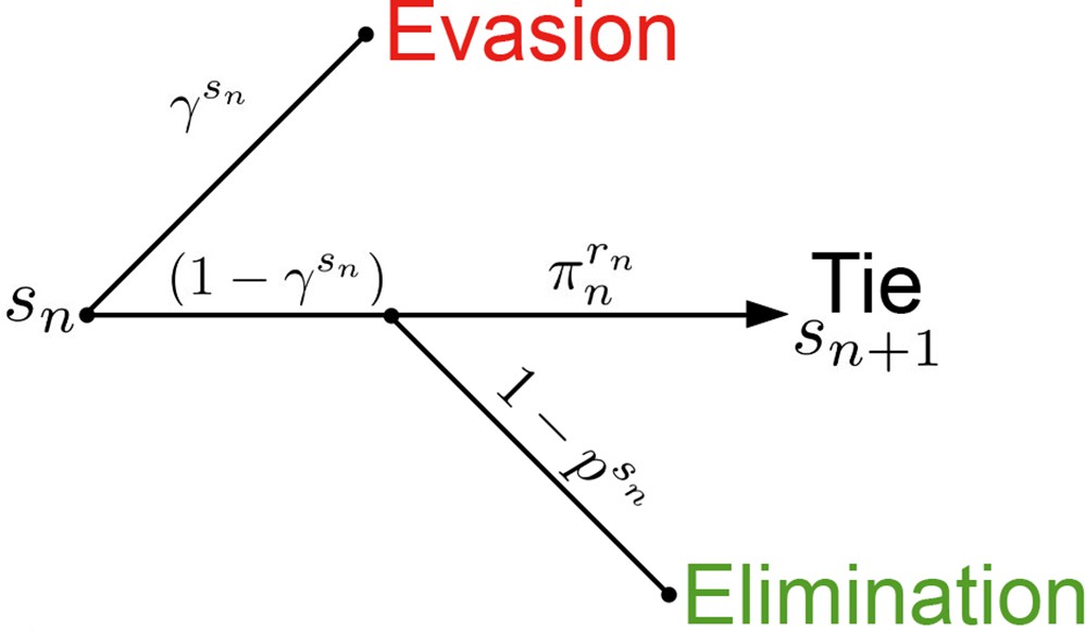
Passive Evader outcome tree.

Figure 1—figure supplement 3

Download asset Open asset

Active Evader decision tree.

This process is identical to that of the Passive Evader case (Figure 1—figure supplement 2), except that in this case the evasion rate $π_{n}$ may be chosen at each period by the Evader.

Figure 1—figure supplement 4

Download asset Open asset

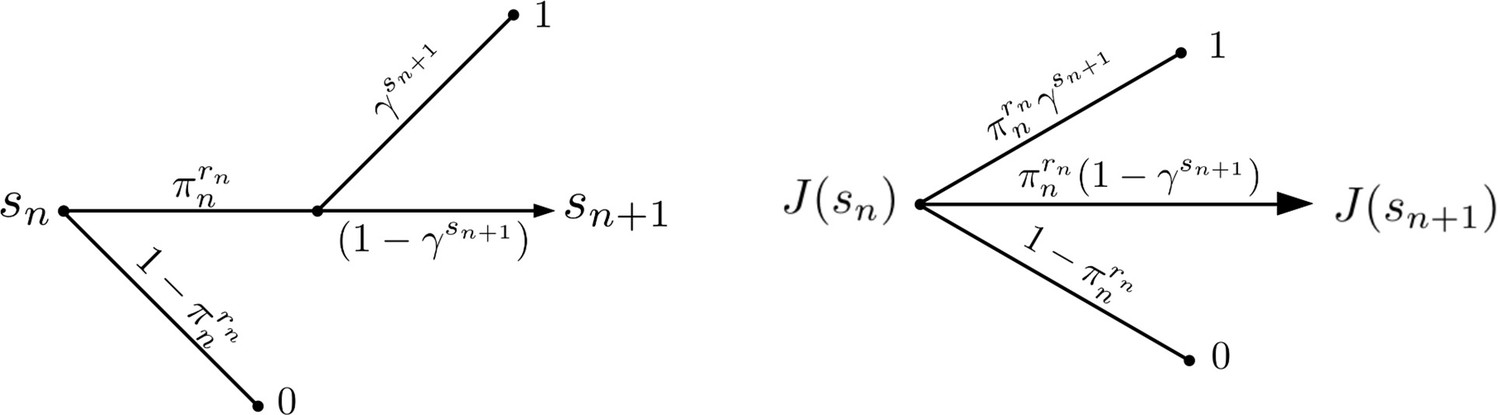
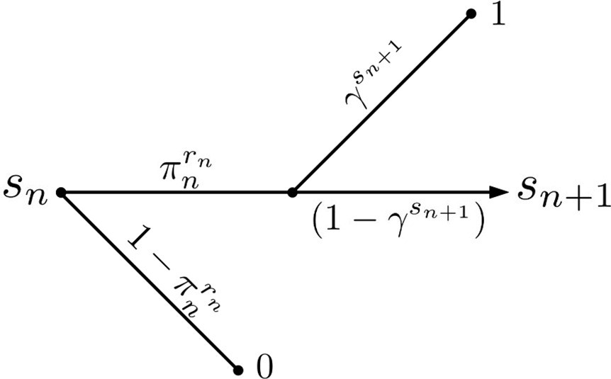
Active Evader reward structure.

The value function for the Evader $J$ is represented under stationary dynamics. The reward of Evader elimination is 0, and for successful escape is assumed to be 1.

Figure 1—figure supplement 5

Download asset Open asset

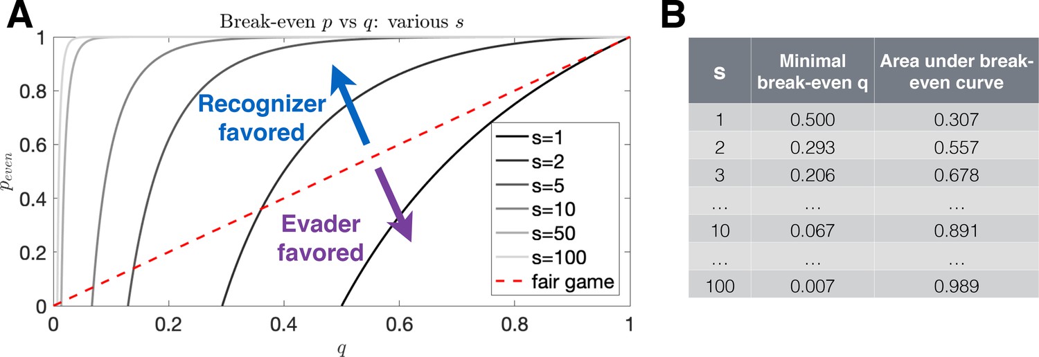
Break-even evasion probability as a function of recognition probability.

(A) The break-even probability is given as a function of recognition probability for various numbers of recognizable antigen. The red dashed line illustrates a fair game, where an equal proportion of parameters favors the Evader and Recognizer. Recognition (resp. evasion) is favored in systems for which the area below the $p_{even}$ curve is large (resp. small). (B) Values for the minimal evasion probabilities allowable for the existence of a break-even probability as well as area under the break-even curve for various antigen numbers.

Figure 1—figure supplement 5—source data 1 Source data contains a spreadsheet of Figure 1—figure supplement 5B table.: https://cdn.elifesciences.org/articles/82786/elife-82786-fig1-figsupp5-data1-v1.xlsx
Download elife-82786-fig1-figsupp5-data1-v1.xlsx

Figure 1—figure supplement 6

Download asset Open asset

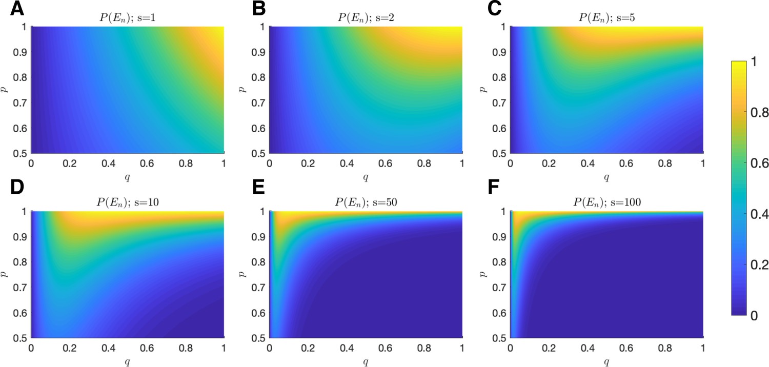
Probability of equilibrium.

The probability of tumor-immune equilibrium is plotted as a function of $q$ (x-axis) and $p$ (y-axis) for (A) $s = 1$ ; (B) $s = 2$ ; (C) $s = 5$ ; (D) $s = 10$ ; (E) $s = 50$ ; and (F) $s = 100$ .

Figure 1—figure supplement 7

Download asset Open asset

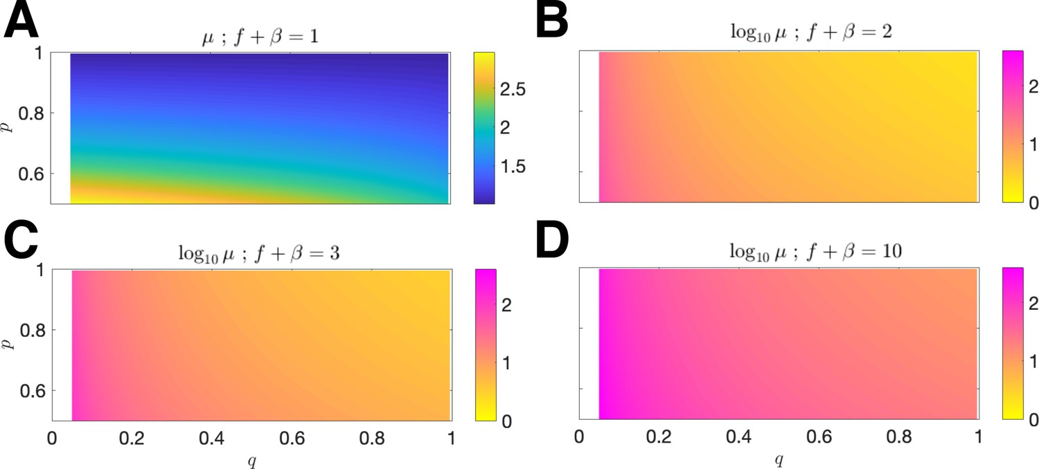
Mean antigenic load at equilibrium.

The mean antigen equilibrium point μ is plotted as a function of $q$ (x-axis) and $p$ (y-axis) for mean penalty (A) $f + β = 1$ ; the normalized $\log_{10} μ$ vs. $q$ and $p$ is plotted for mean penalty; (B) $f + β = 2$ ; (C) $f + β = 3$ ; (D) $f + β = 10$ (in all cases, the relevant domain is restricted to $(p, q) \in (0.5, 1) \times (0.05, 1)$ ).

Figure 1—figure supplement 8

Download asset Open asset

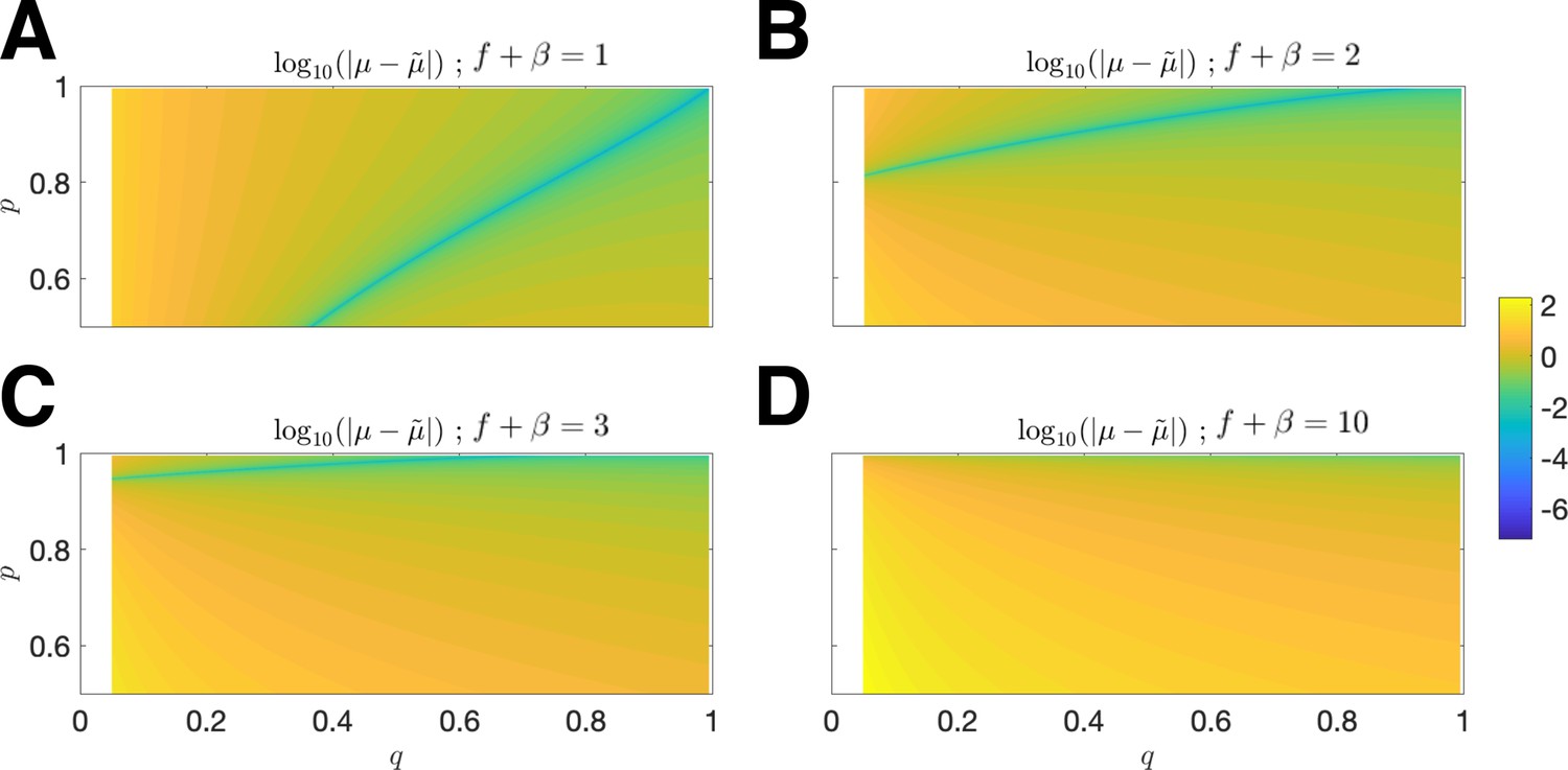
Error of upper estimate $\tilde{μ}$ .

The log-absolute error $\log_{10} (| μ - \tilde{μ} |)$ vs. $q$ and $p$ is plotted for mean penalty (A) $f + β = 1$ ; (B) $f + β = 2$ ; (C) $f + β = 3$ ; (D) $f + β = 10$ (in all cases, the relevant domain is restricted to $(p, q) \in (0.5, 1) \times (0.05, 1)$ ).

Figure 1—figure supplement 9

Download asset Open asset

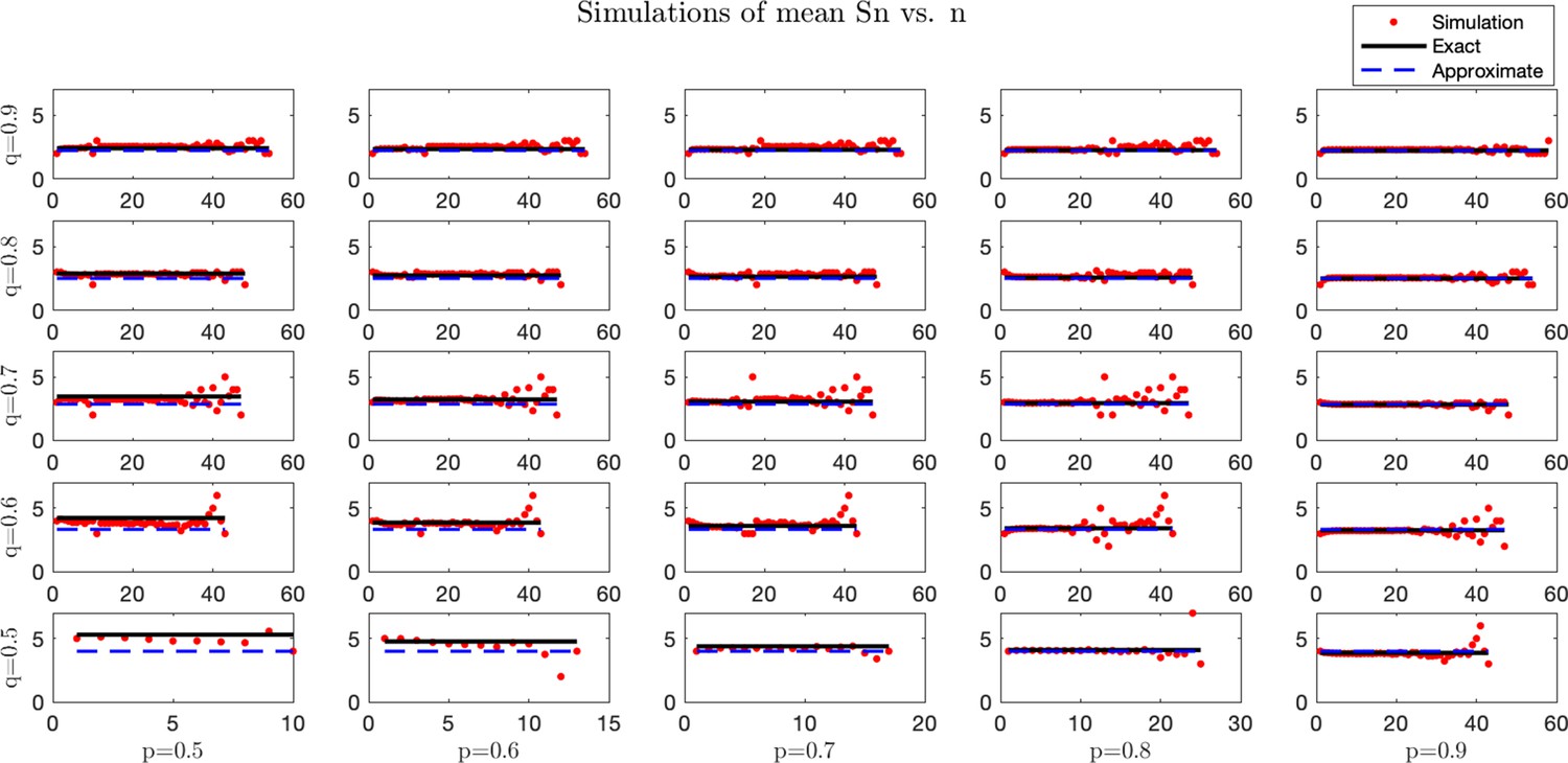
Simulated and analytical mean antigenic load at equilibrium.

Stochastic simulations were performed for a process with $s_{0}$ set equal to the rounded predicted μ. For each trajectory, the pre-escape/elimination time and number of antigens are recorded, and an average is taken for each time. Simulation averages (red) are compared with predicted exact (black solid line) and approximate (blue dashed line) mean dynamics. For each case, $n = 10^{6}$ simulations were performed under small mean penalty $f + β = 2$ . Columns from left-to-right correspond with $p \in {0.5, 0.6, 0.7, 0.8, 0.9}$ . Rows from bottom-to-top correspond with $q \in {0.5, 0.6, 0.7, 0.8, 0.9}$ .

Figure 1—figure supplement 10

Download asset Open asset

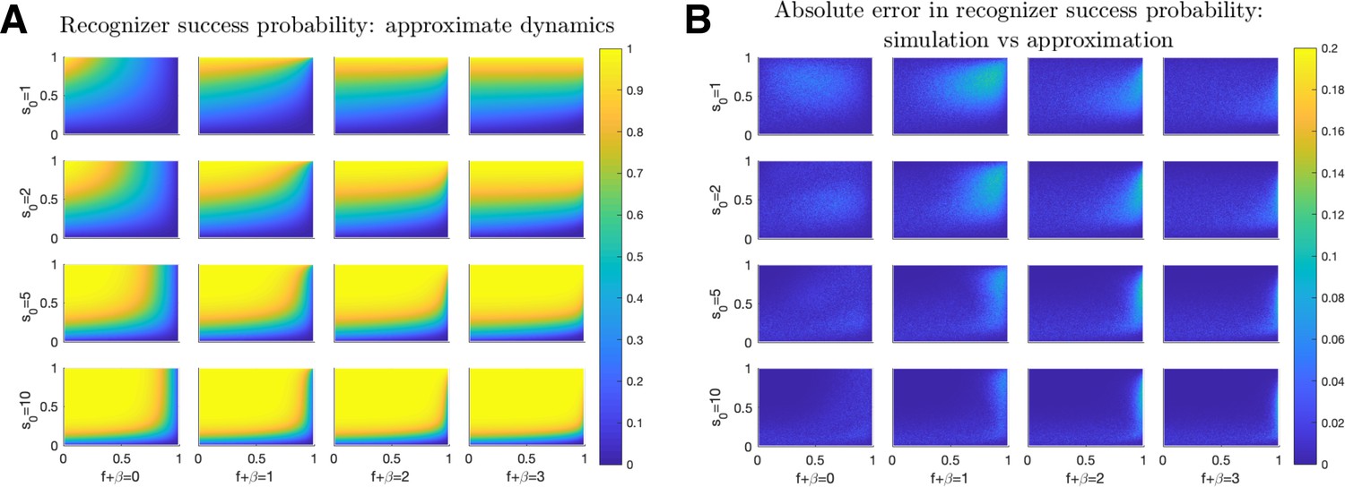
Probability of Recognizer success.

Recognizer success probabilities are plotted as a function of $p$ ( $x$ -axis) and $q$ ( $y$ -axis) for (A) approximate dynamics (Equation 31). (B) The absolute difference between the above approximations and simulated exact (Equation 3) dynamics. Results averaged over 1000 iterations for each $(q, p, s_{0}, f + β)$ quintuplet. Columns from left-to-right correspond with $f + β \in {0, 1, 2, 3}$ . Rows from top-to-bottom correspond with $s_{0} \in {1, 2, 5, 10}$ .

Figure 1—figure supplement 11

Download asset Open asset

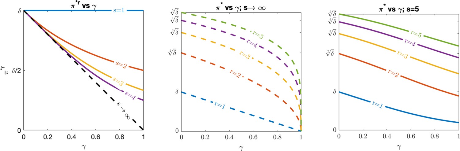
Optimal evasion.

(Left) $π^{*} r$ vs. $γ$ , (middle) $π^{*}$ vs. $γ$ for $s \to \infty$ , and (right) $π^{*}$ vs. $γ$ for $s = 5$ under various values of recognized antigens, assuming $δ < 1$ .

Figure 2

Download asset Open asset

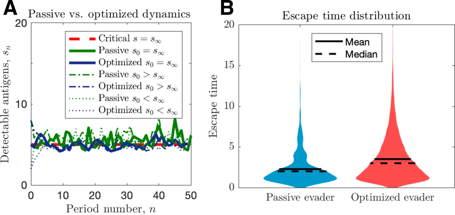
Passive and optimized evasion strategies against stationary threats.

(A) Comparisons of the temporal dynamics of passive (green) and active (blue) strategies with parameter selections giving equal mean behavior. In the active case, $q = q^{*} + 0.1$ yields stable dynamics, giving mean antigen arrival $β + f = 3.44$ . In the passive case, $p = 0.90$ was selected to match the mean optimal evasion rate and the expected s_n of the active case. Also, $f = 3.51$ and $β = 0.88$ both chosen so that $s_{\infty} = 5$ , and the results plotted for s₀ $\in {2, 5, 8}$ {2, 5, 8}. (B) 10⁶ replicates of this process were used to calculate distributions of stopping times conditioned on escape. This distribution generates passive (resp. optimized) $p_{escape}$ of 5.37 (resp. 8.44).

Figure 2—source data 1 Source data contains a spreadsheet of data for Figure 2B.: https://cdn.elifesciences.org/articles/82786/elife-82786-fig2-data1-v1.xlsx
Download elife-82786-fig2-data1-v1.xlsx

Figure 3

Download asset Open asset

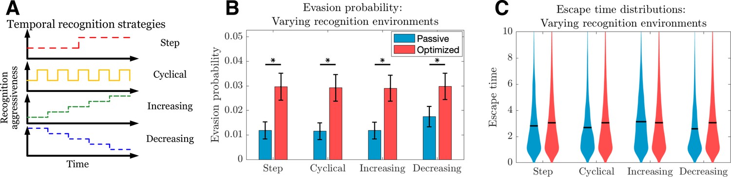
Passive and optimized evasion strategies for temporally varying recognition profiles.

(A) Temporally varying recognition functions are selected and applied to threats employing passive (blue) and optimized (red) evasion strategies. (B) The mean and standard deviation of escape probabilities is compared across recognition profiles for each strategy (pairwise significance was assessed using two-sample t-test at significance $α = 0.05$ with $p$ <10^-5). (C) Escape time distributions are generated for step, cyclical, increasing, and decreasing recognition environments (solid line: mean). In each case, mean total new antigen arrival $β + E [f_{n}]$ for passive (resp. optimized) evasion were 4.39 (resp. 4.75), and 10³ simulations of 10³ replicates each were used for statistical comparison; all samples were aggregated for escape time violin plots (solid line denotes mean).

Figure 3—source data 1 Source data contains a spreadsheet of data for Figure 3B, C.: https://cdn.elifesciences.org/articles/82786/elife-82786-fig3-data1-v1.xlsx
Download elife-82786-fig3-data1-v1.xlsx

Figure 4

Download asset Open asset

Distribution of available post-escape tumor antigens.

The distribution of tumor-associated antigens (TAAs) was estimated from simulations of optimized cancer evasion resulting in escape and plotted for (A) increasing recognition probability $q \in {0.6, 0.65, 0.7, 0.75, 0.8, 0.85, 0.9, 0.95}$ and (B) increasing evasion penalty $β \in {0.1, 0.2, 0.3, 0.4, 0.5, 0.6, 0.7, 0.8}$ . For (A), $β = 0.59$ . For (B), $q = 0.7 > q^{*}$ . In both cases, $s_{\infty} = 5$ and $n = 10^{6}$ simulations were performed for each histogram.

Figure 4—source data 1 Source data contains a spreadsheet of data for Figure 4A, B.: https://cdn.elifesciences.org/articles/82786/elife-82786-fig4-data1-v1.xlsx
Download elife-82786-fig4-data1-v1.xlsx

Figure 5 with 4 supplements

Download asset Open asset

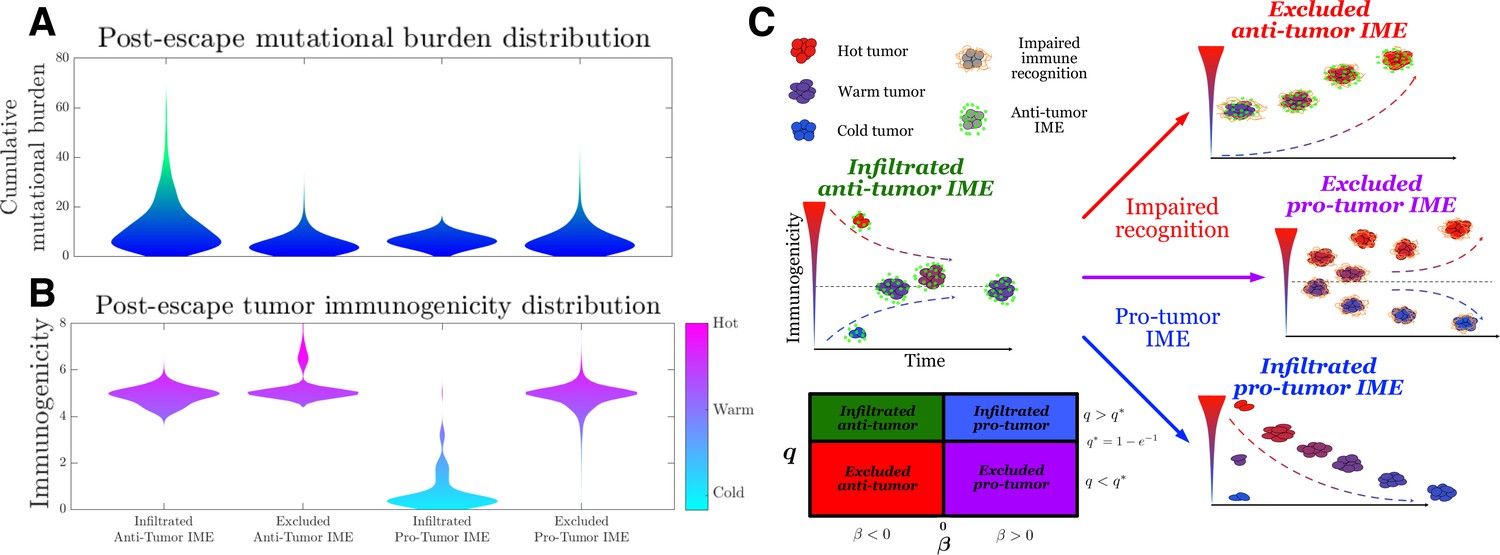
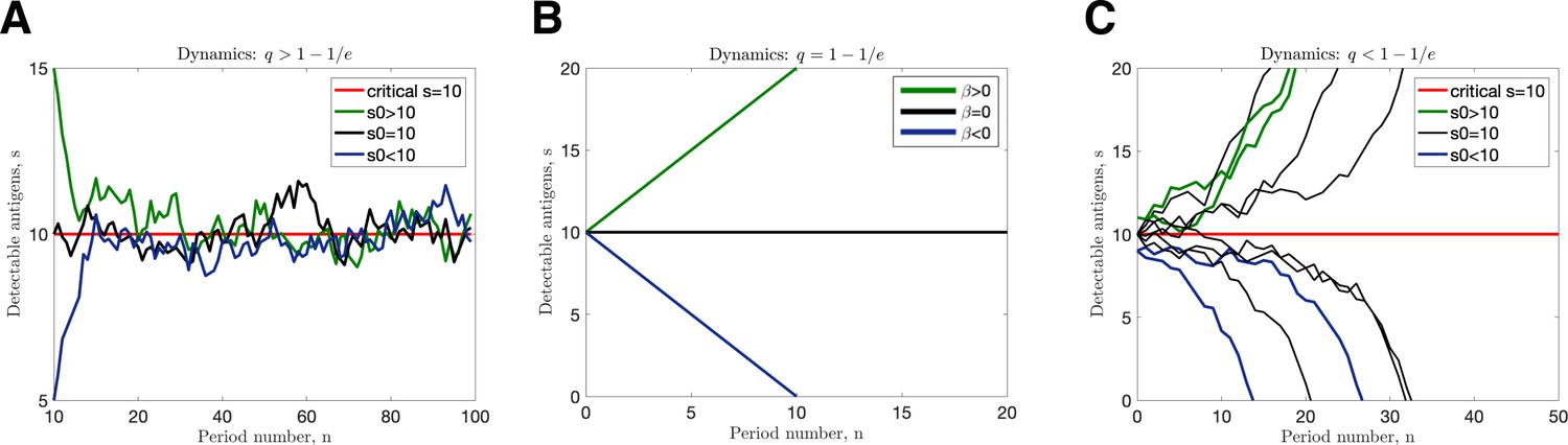
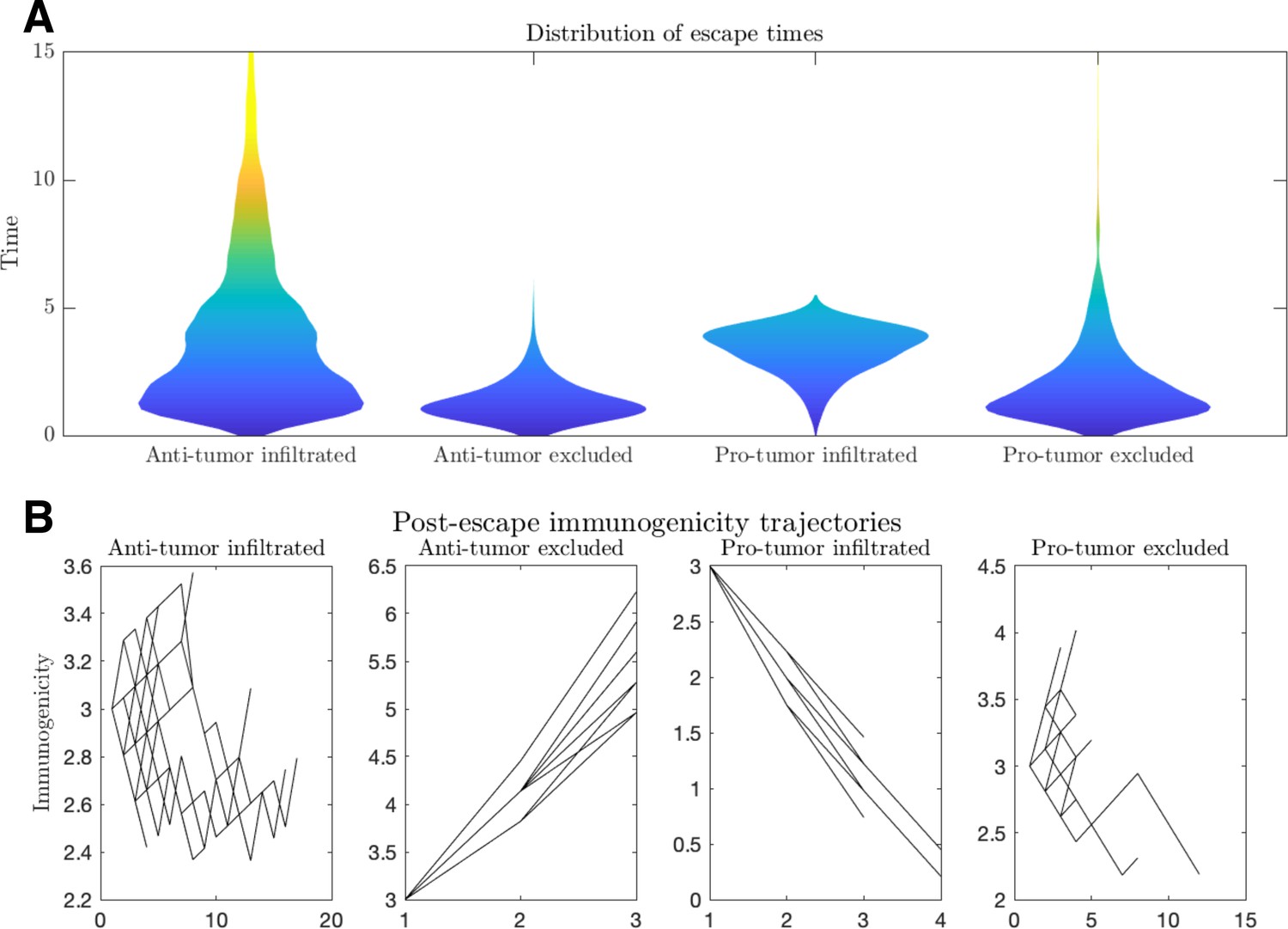
Active Evader dynamics.

Violin plots of the distribution of post-immune escape. (A) Cumulative mutation burden. (B) Post-escape immunogenicity (available tumor-associated antigens [TAAs]) as a function of time for a variety of tumor immune microenvironment (IME) conditions. (Anti-tumor-infiltrated: $q = q^{*} + 0.1$ , $β = 0.529$ ; anti-tumor-excluded: $q = q^{*} - 0.1$ , $β = 0.505$ ; pro-tumor-infiltrated: $q = q^{*} + 0.1$ , $β = - 0.529$ ; pro-tumor-excluded: $q = q^{*} - 0.1$ , $β = - 0.505$ . In all cases, $β$ chosen to give $| s_{\infty} | = 3$ [ $s_{\infty} = - 3$ for the pro-tumor-infiltrated case] giving strictly positive penalties. Simulations were run until $n = 10^{6}$ escape events occurred for each case.) (C) The number of recognizable TAAs over time along with equilibrium states is depicted assuming (left) anti-tumor IME, $β > 0$ , and efficient immune recognition. Compromises in (top right) recognition, $q < q^{*}$ ; (bottom right) the establishment of a pro-tumor IME, $β < 0$ , or (middle right) both affect the predicted dynamical behavior of tumor immunogenicity. A phase plot partitions each case as a function of relevant critical parameter values.

Figure 5—source data 1 Source data contains a spreadsheet of data for Figure 5A, B.: https://cdn.elifesciences.org/articles/82786/elife-82786-fig5-data1-v1.xlsx
Download elife-82786-fig5-data1-v1.xlsx

Figure 5—figure supplement 1

Download asset Open asset

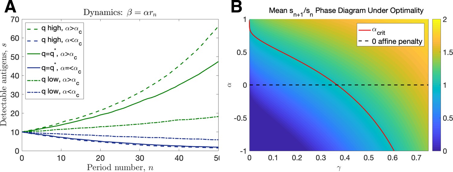
Linear dynamics.

(A) Simulated trajectories assuming $β = α r_{n}$ ( $q$ high: $q = 0.75$ , $q^{*} = 1 - 1 / e$ , $q$ low: $q = 0.25$ , $α_{c}$ given by Equation 86, $α < α_{c}$ ). (B) Mean intertemporal gain as a function of $γ = 1 - q$ and $α$ .

Figure 5—figure supplement 2

Download asset Open asset

Transition dynamics.

(A) $q > q^{*}$ and $β = 1.76$ ; (B) $q = q^{*}$ ; (C) $q < q^{*}$ and $β = - 1.68$ (in all cases illustrated, $β$ chosen so that $s^{*} = 10$ ).

Figure 5—figure supplement 3

Download asset Open asset

Escape dynamics.

(A) Violin plots of the distribution of escape times and (B) immunogenicity (number of relevant tumor-associated antigens [TAAs]) as a function of time for a variety of tumor microenvironmental conditions. (Anti-tumor-infiltrated: $q = q^{*} + 0.1$ , $β = 0.529$ ; anti-tumor-excluded: $q = q^{*} - 0.1$ , $β = 0.505$ ; pro-tumor-infiltrated: $q = q^{*} + 0.1$ , $β = - 0.529$ ; pro-tumor-excluded: $q = q^{*} - 0.1$ . $β = - 0.505$ . In all cases, $β$ chosen to give. $| s^{*} | = 3$ . Simulations were run until $n = 10^{6}$ escape events occurred for each case. Plot B trajectories were obtained by plotting the immunogenicity trajectories for 50 post-escape events at each time point $n$ for which $n \geq 2$ .)

Figure 5—figure supplement 4

Download asset Open asset

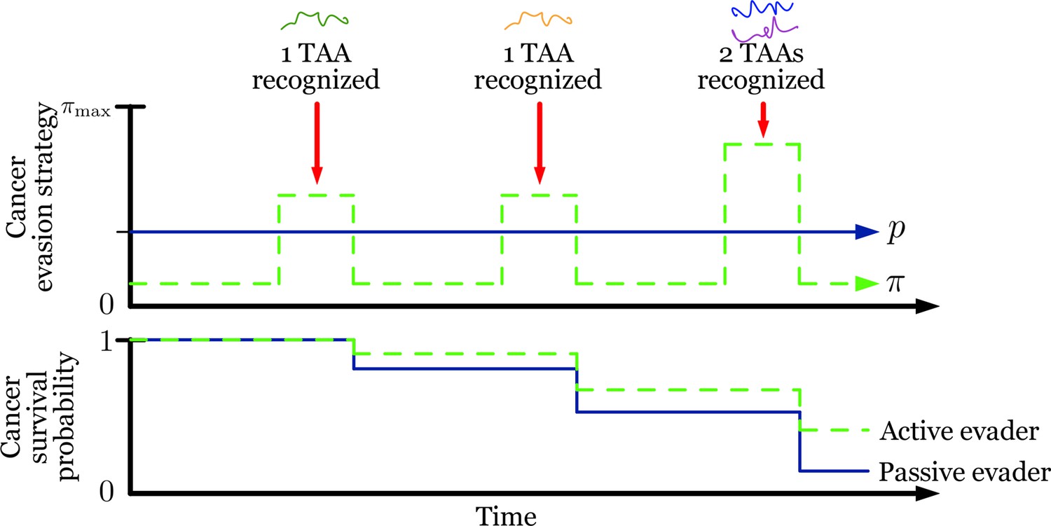
Active evasion summary.

Summary of optimized adaptive vs. passive evasion on temporally varying recognition and their effect on overall cancer survival.

Additional files

MDAR checklist: https://cdn.elifesciences.org/articles/82786/elife-82786-mdarchecklist1-v1.pdf
Download elife-82786-mdarchecklist1-v1.pdf

Download links

A two-part list of links to download the article, or parts of the article, in various formats.

Downloads (link to download the article as PDF)

Open citations (links to open the citations from this article in various online reference manager services)

Mendeley

Cite this article (links to download the citations from this article in formats compatible with various reference manager tools)

Jason T George
Herbert Levine

(2023)

Optimal cancer evasion in a dynamic immune microenvironment generates diverse post-escape tumor antigenicity profiles

eLife 12:e82786.

https://doi.org/10.7554/eLife.82786

Sign up for email alerts

Privacy notice