Thermal phenotypic plasticity of pre- and post-copulatory male harm buffers sexual conflict in wild Drosophila melanogaster
- Ethology Lab, Cavanilles Institute of Biodiversity and Evolutionary Biology, University of Valencia, Spain
- Department of Biology, Lund University, Sweden
Figures
Figure 1 with 5 supplements
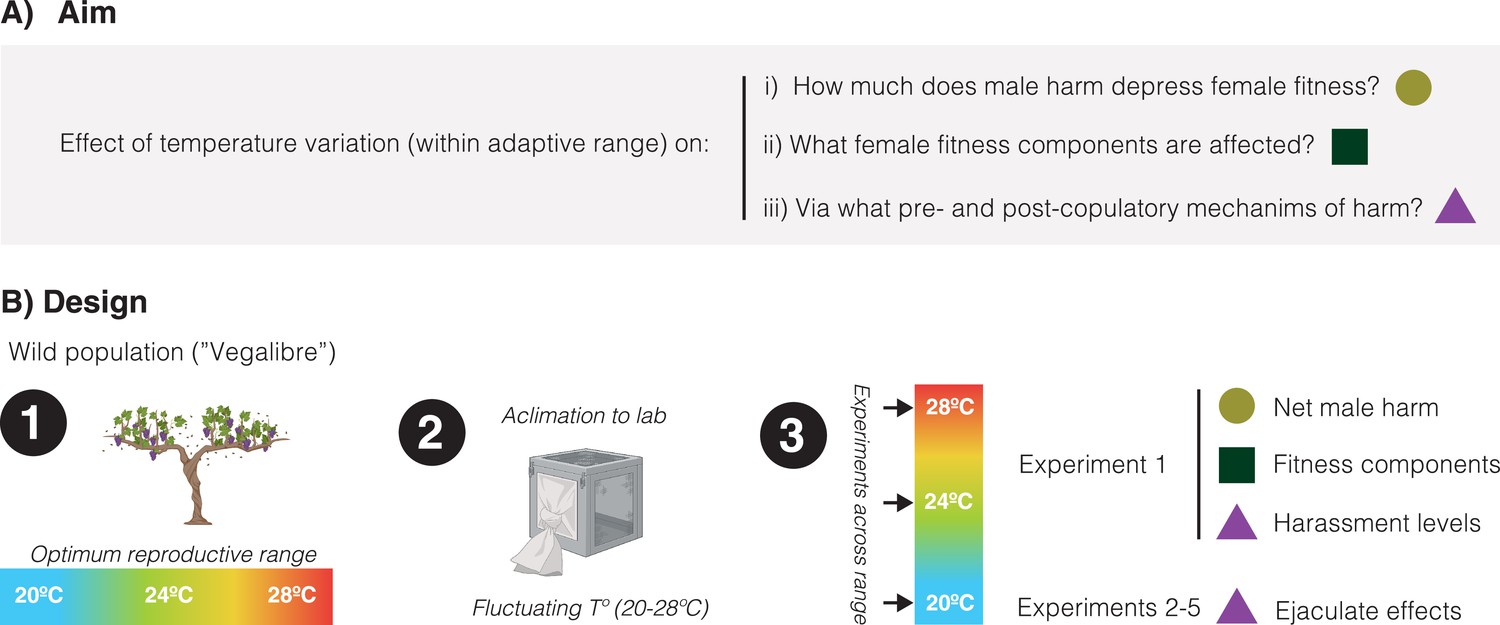
Schematic overview of the study.
(A) Our aim was to study how temperature variation, across a range at which reproduction is optimum in the wild, may affect: the net decrease in female fitness resulting from male harm, what female fitness components are mainly affected by male harm, and pre-copulatory (i.e. sexual harassment) and post-copulatory (i.e. ejaculate effects on female receptivity, short-term fecundity, and survival) mechanism of harm. (B) General design of the study: (1) We sampled a wild population of Drosophila melanogaster flies that reproduce optimally between 20°C and 28°C, (2) We setup a population in the lab and left it to acclimate for a few generations under a programmed fluctuating temperature regime that mimics wild conditions in late spring-early summer (20–28°C range with mean at 24°C), (3) We run a series of five experiments (each repeated at 20°C, 24°C, and 28°C) to study temperature effects on net male harm, female fitness components and male pre- and post-copulatory mechanisms of harm.
Figure 1—figure supplement 1
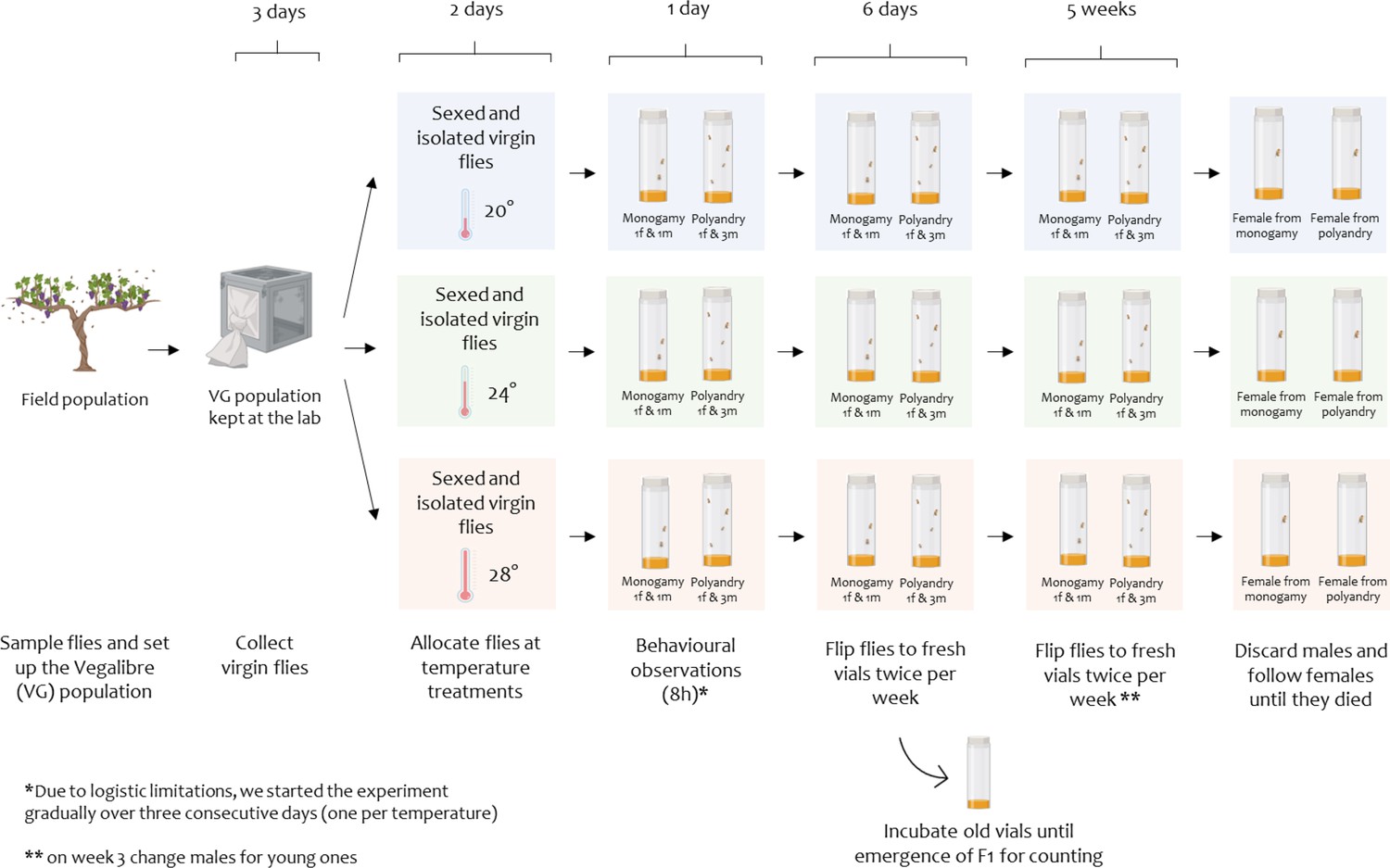
Fitness and behavioural assay design (Experiment 1).
Figure 1—figure supplement 2

Receptivity assay design (Short treatment duration – 48 hr, experiment 2).
Figure 1—figure supplement 3
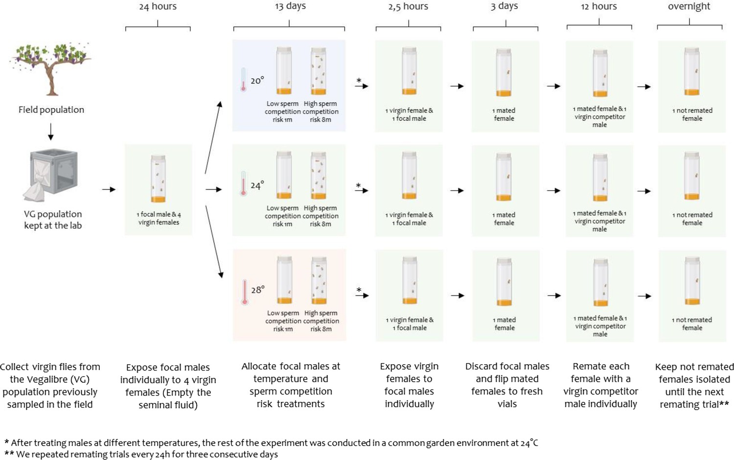
Receptivity assay design (Long treatment duration – 13 days, experiment 3).
Figure 1—figure supplement 4

Fecundity and survival assay design (Short treatment duration – 48 hr, experiment 4).
Figure 1—figure supplement 5
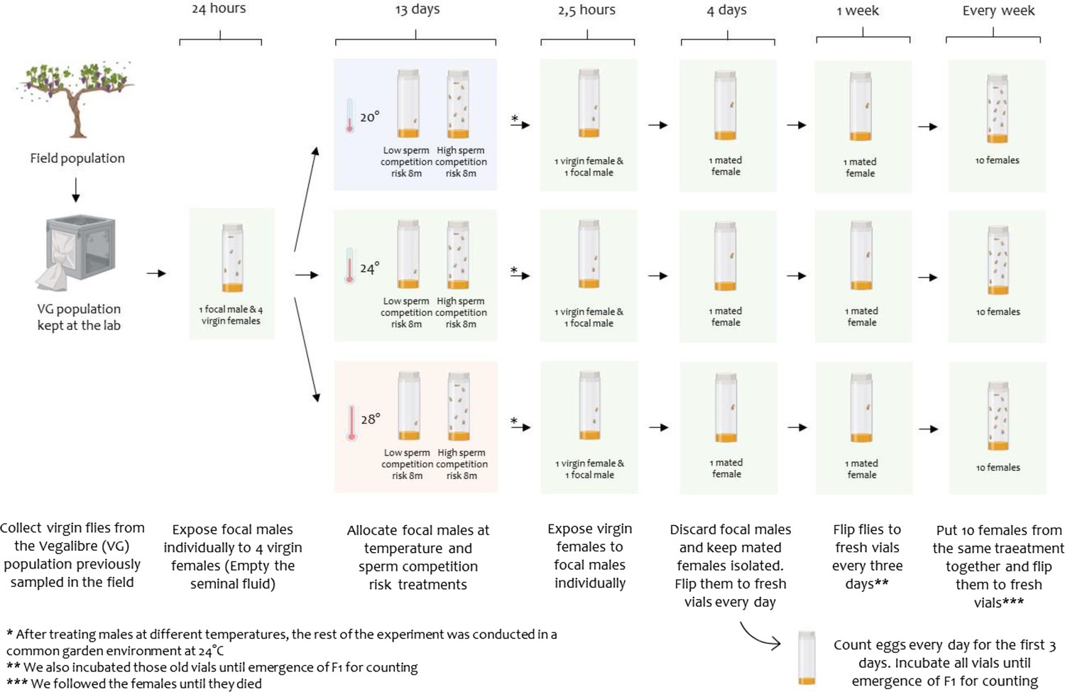
Fecundity and survival assay design (Long treatment duration – 13 days, experiment 5).
Figure 2 with 2 supplements
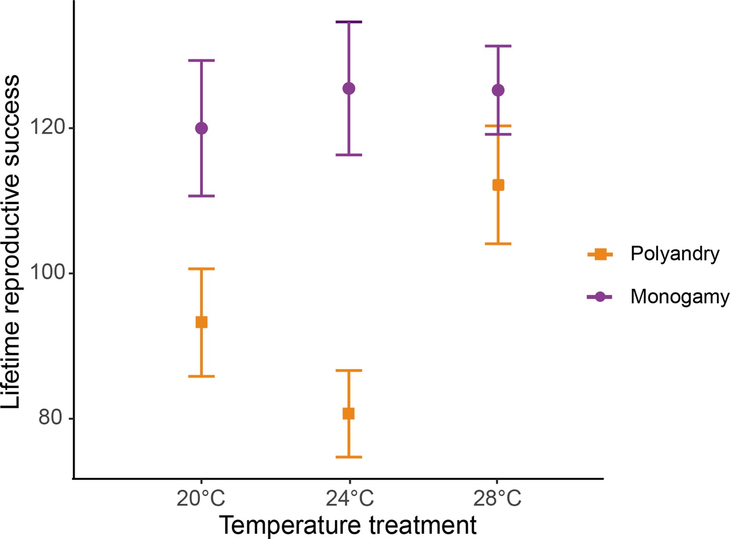
Female lifetime reproductive success (mean ± SEM) across temperature and mating system treatments.
20°C: npolyandry = 73 and nmonogamy = 74. 24°C: npolyandry = 71 and nmonogamy = 74. 28°C: npolyandry = 66 and nmonogamy = 71.
Figure 2—figure supplement 1
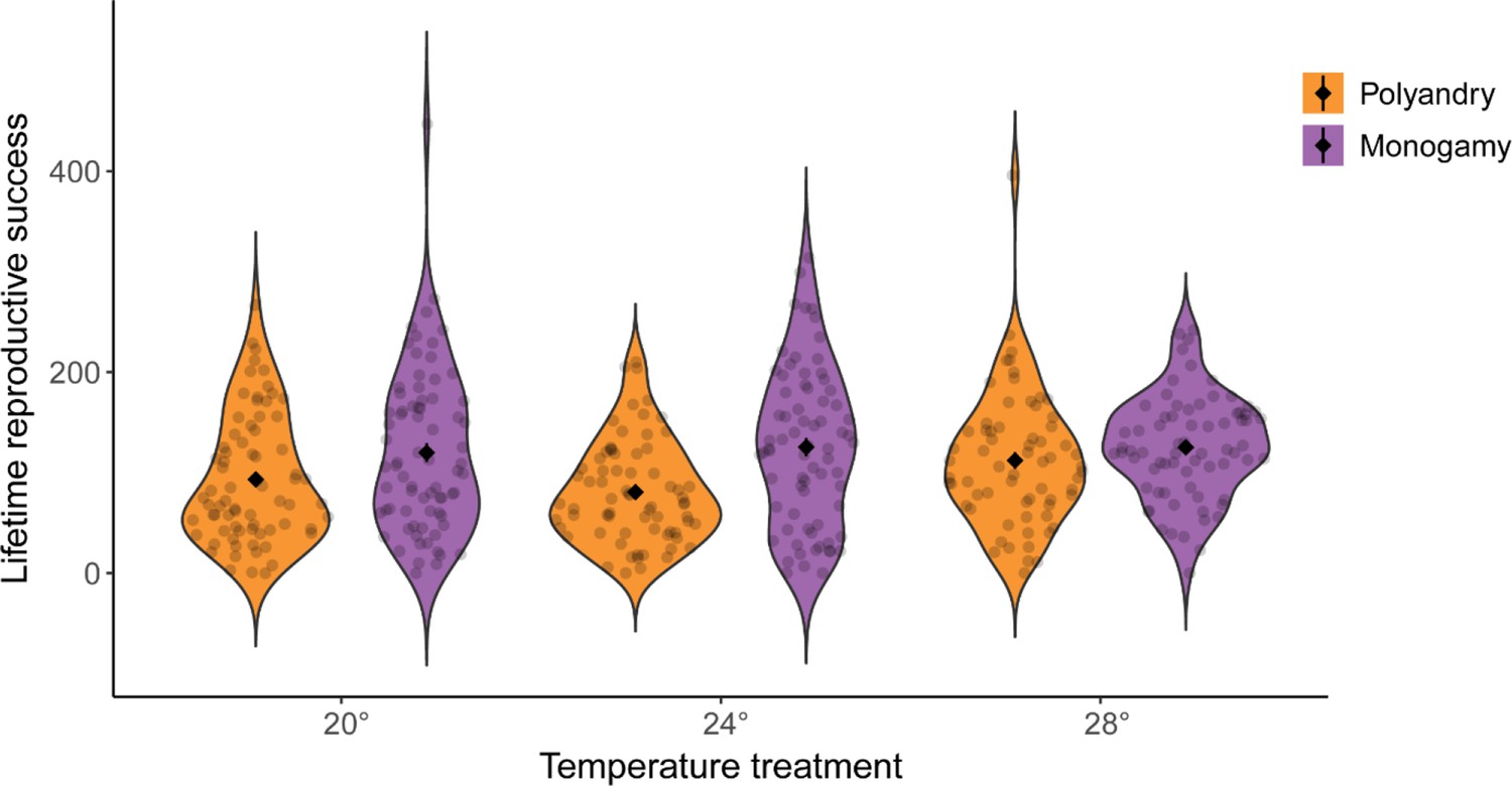
Violin plot for female reproductive success across temperature and mating system treatments.
Figure 2—figure supplement 2
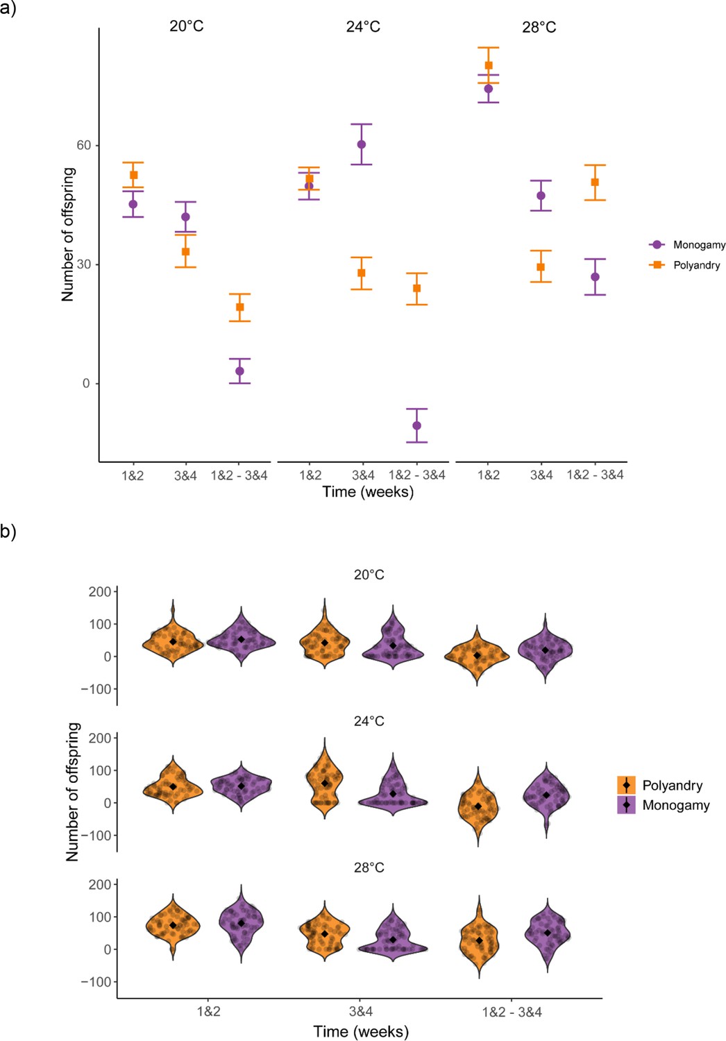
Early reproductive rate (number of offspring produced during the first two weeks of age), late reproductive rate (number of offspring produced during the second two weeks of age), and reproductive aging (number of offspring produced over weeks 1–2 vs. 3-4) plots.
(a) Mean ± SEM number of offspring in monogamy vs. polyandry mating system treatments, across the different temperature treatments. 20°C: npolyandry = 73 and nmonogamy = 74. 24°C: npolyandry = 71 and nmonogamy = 74. 28°C: npolyandry = 66 and nmonogamy = 71. (b) Violin plots.
Figure 3
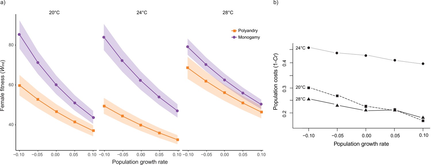
Rate-sensitive fitness estimates.
(a) Average rate-sensitive index fitness estimate of individual females (Mean ωind) for different population growth rates across temperature and mating system treatments (shaded areas denote SEM). 20°C: npolyandry = 73 and nmonogamy = 74. 24°C: npolyandry = 71 and nmonogamy = 74. 28°C: npolyandry = 66 and nmonogamy = 71. (b) Relative cost (Cr) of polyandry (vs. monogamy) for each temperature treatment for different population growth rates. Cr was calculated based on rate-sensitive index fitness estimates for populations (ωpop), whereby population costs are shown as 1 – Cr, thus reflecting the relative decrease in population growth rate.
Figure 4 with 1 supplement
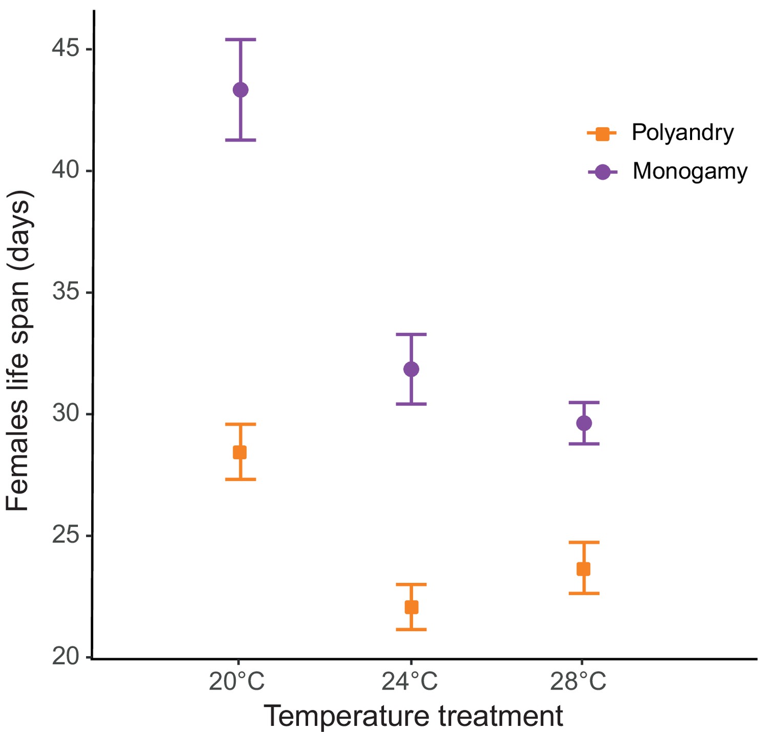
Male harm effect on female lifespan (mean ± SEM) across temperature and mating system treatments.
20°C: npolyandry = 73 and nmonogamy = 74. 24°C: npolyandry = 71 and nmonogamy = 73. 28°C: npolyandry = 66 and nmonogamy = 73.
Figure 4—figure supplement 1
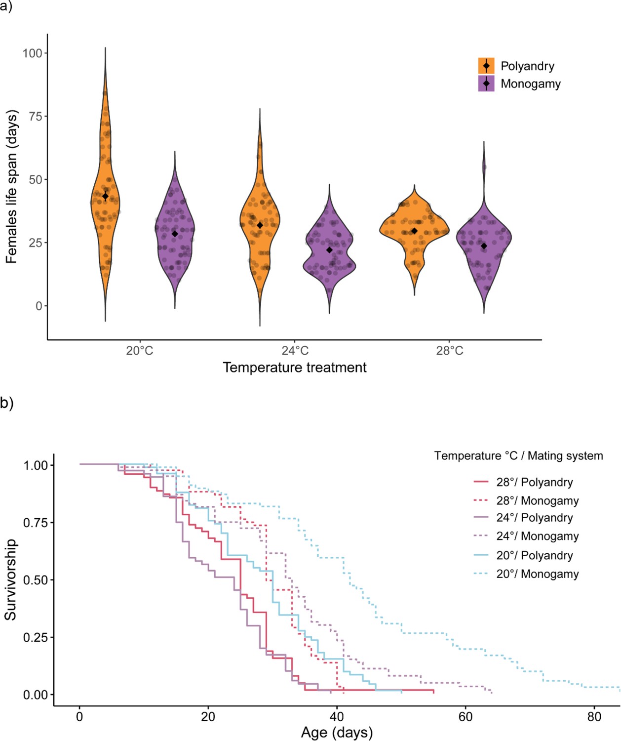
Male harm effect on female lifespan across temperature and mating system treatments.
(a) Violin plot. (b) Survival plot from the Cox proportional hazard model as a complementary analysis.
Figure 5 with 2 supplements
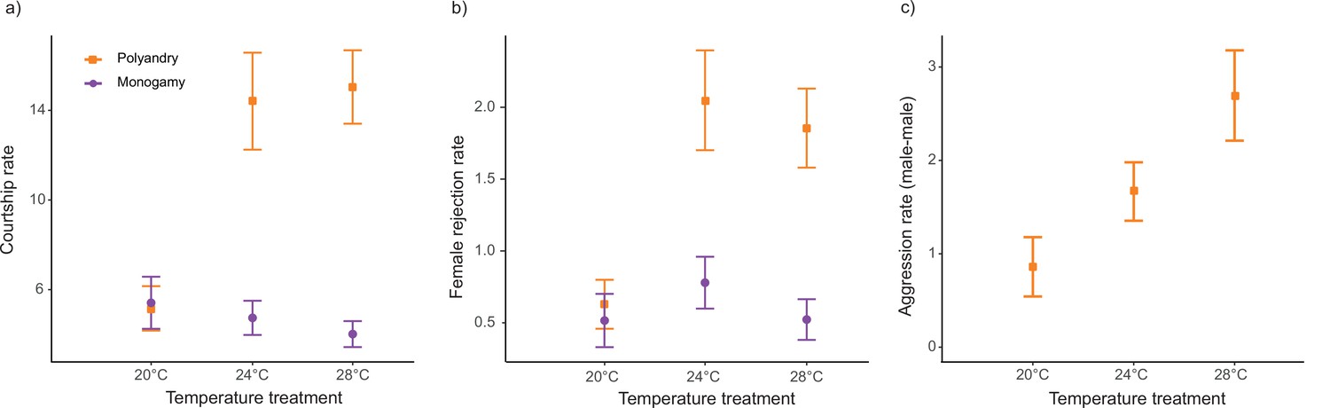
Reproductive behaviors (mean ± SEM) across temperature and mating system treatments.
(a) Courtships per female per hour, (b) Female rejections per hour, and (c) Aggressions male-male per hour. 20°C: npolyandry = 74 and nmonogamy = 76. 24°C: npolyandry = 72 and nmonogamy = 77. 28°C: npolyandry = 70 and nmonogamy = 75.
Figure 5—figure supplement 1
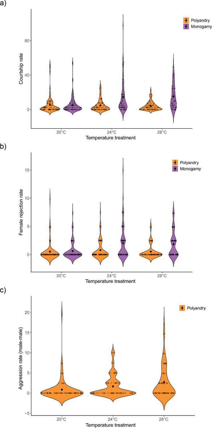
Violin plot for male harm effect on: (a) Courtship rate and (b) Rejection rate across temperature and mating system treatments; (c) Violin plot for polyandry mating system effect on aggression rate.
Figure 5—figure supplement 2
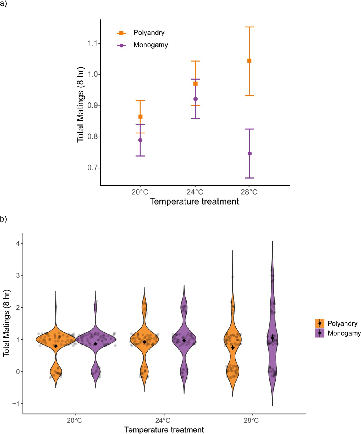
Total number of matings across the 8 hr of observations.
(a) Mean ± SEM across temperature and mating system treatments. (b) Violin plot. Data from reproductive behaviour measures. 20°C: npolyandry = 74 and nmonogamy = 76. 24°C: npolyandry = 72 and nmonogamy = 77. 28°C: npolyandry = 70 and nmonogamy = 75.
Figure 6 with 4 supplements
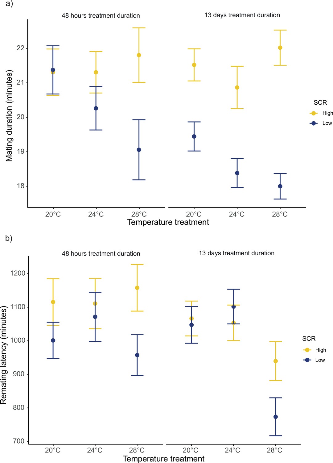
Mean ± SEM for mating duration and remating latency.
(a) Mating duration of males exposed to high (8 males per vial) or low sperm competition risk (1 male per vial) for 48 hr or 13 days prior to mating at different temperatures. 20°C: nhigh/48hr = 91, nlow/48hr = 96, nhigh/13days = 121 and nlow/13days = 117. 24°C: nhigh/48hr = 85, nlow/48hr = 88, nhigh/13days = 119 and nlow/13days = 115. 28°C: nhigh/48hr = 92, nlow/48hr = 104, nhigh/13days = 99 and nlow/13days = 117. (b) Female remating latency following a single mating with either a male from a high or low sperm competition risk level for 48 hr or 13 days before mating across temperature treatments. 20°C: nhigh/48hr = 75, nlow/48hr = 73, nhigh/13days = 119 and nlow/13days = 113. 24°C: nhigh/48hr = 61, nlow/48hr = 70, nhigh/13days = 116 and nlow/13days = 113. 28°C: nhigh/48hr = 63, nlow/48hr = 82, nhigh/13days = 98 and nlow/13days = 117.
Figure 6—figure supplement 1

Violin plots for (a) Mating duration of males exposed to a high (8 males per vial) or low sperm competition risk (1 male per vial) level 48 hr (experiment 2) and 13 days (experiment 3) before mating across temperature treatments, and (b) Female remating latency following a single mating with either a male from a high or low sperm competition risk level, for both 48 hr and 13 days of temperature treatment duration before mating in a common garden.
Figure 6—figure supplement 2
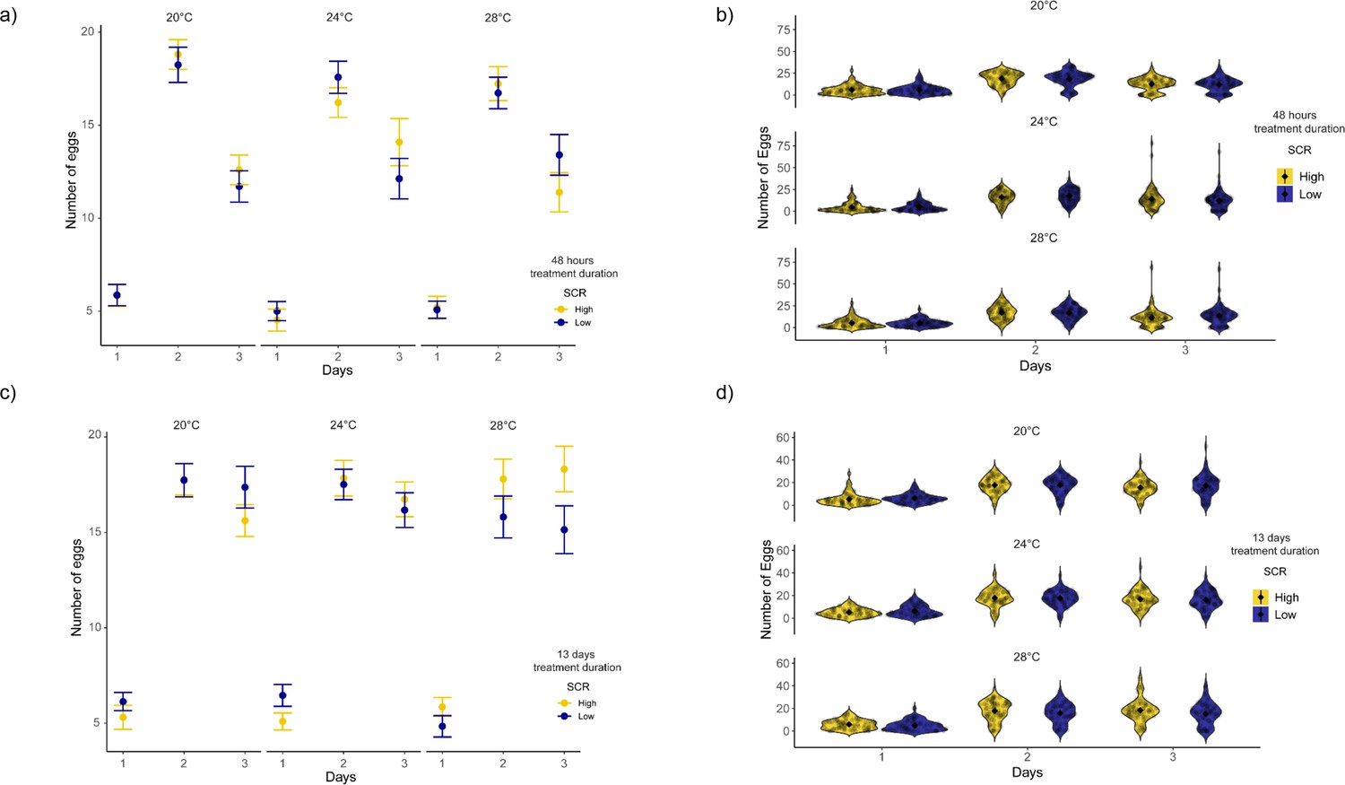
Eggs produced by females during the first three days following a single mating with treated males.
(a) Mean ± SEM, 48 hr treatment duration. 20°C: nhigh/day 1 = 88, nlow/day 1 = 86, nhigh/day 2 = 88, nlow/day 2 = 86, nhigh/day 3 = 88 and nlow/day 3 = 86. 24°C: nhigh/day 1 = 87, nlow/day 1 = 88, nhigh/day 2 = 87, nlow/day 2 = 88, nhigh/day 3 = 87 and nlow/day 3 = 88. 28°C: nhigh/day 1 = 86, nlow/day 1 = 86, nhigh/day 2 = 86, nlow/day 2 = 86, nhigh/day 3 = 86 and nlow/day 3 = 86. (b) Violin plot, 48 hr treatment duration. (c) Mean ± SEM, 13 days treatment duration. 20°C: nhigh/day 1 = 74, nlow/day 1 = 76, nhigh/day 2 = 74, nlow/day 2 = 76, nhigh/day 3 = 74 and nlow/day 3 = 76. 24°C: nhigh/day 1 = 72, nlow/day 1 = 76, nhigh/day 2 = 72, nlow/day 2 = 76, nhigh/day 3 = 72 and nlow/day 3 = 76. 28°C: nhigh/day 1 = 75, nlow/day 1 = 65, nhigh/day 2 = 75, nlow/day 2 = 63, nhigh/day 3 = 75 and nlow/day 3 = 63. (d) Violin plot, 13 days treatment duration.
Figure 6—figure supplement 3
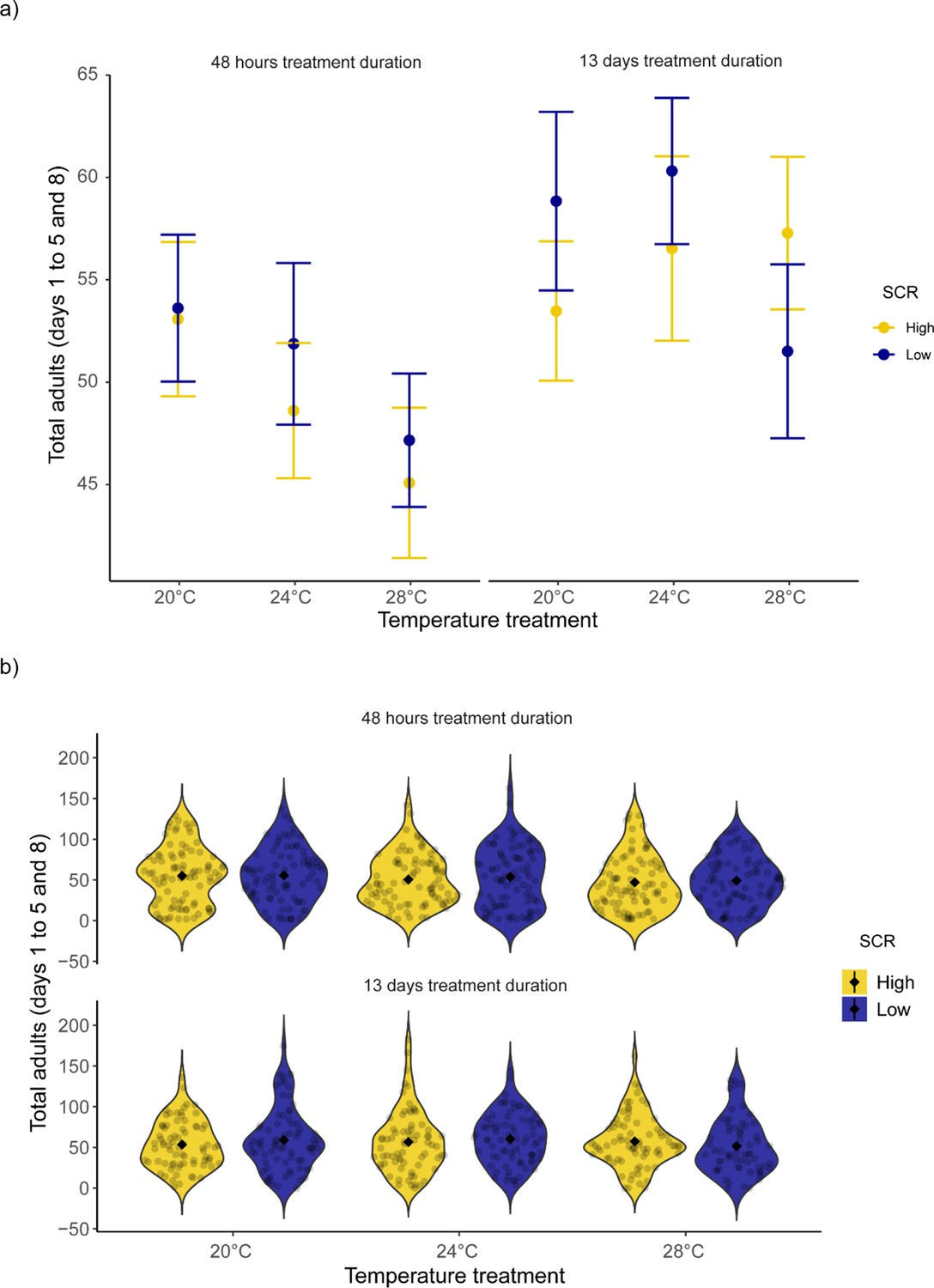
Total of offspring produced by females during the days 1, 2, 3, 4, 5, and 8 after mating following a single mating with treated males.
(a) Mean ± SEM. 20°C: nhigh/48hr = 88, nlow/48hr = 86, nhigh/13days = 74 and nlow/13days = 76. 24°C: nhigh/48hr = 87, nlow/48hr = 88, nhigh/13days = 72 and nlow/13days = 76. 28°C: nhigh/48hr = 86, nlow/48hr = 86, nhigh/13days = 75 and nlow/13days = 63.(b) Violin plot.
Figure 6—figure supplement 4
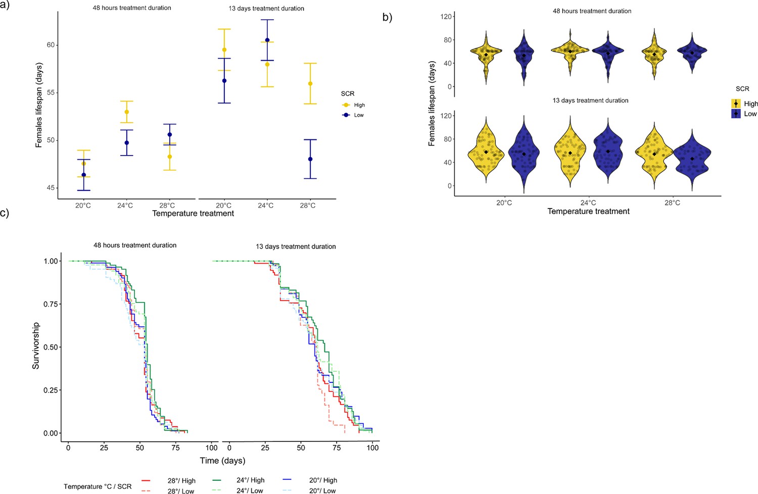
Female lifespan after mating following a single mating with treated males.
(a) Mean ± SEM. 20°C: nhigh/48hr = 80, nlow/48hr = 80, nhigh/13days = 71 and nlow/13days = 70. 24°C: nhigh/48hr = 81, nlow/48hr = 82, nhigh/13days = 60 and nlow/13days = 73. 28°C: nhigh/48hr = 80, nlow/48hr = 84, nhigh/13days = 69 and nlow/13days = 45. (b) Violin plot (c) Survival plot from the Cox proportional hazard model.
Tables
Table 1
Output from separate generalized linear models (GLMs) for each temperature level to explore significant interactions between temperature and mating system effects on female fitness components.
| T°C | LRS | Reproductive aging | Actuarial aging | ||||||
|---|---|---|---|---|---|---|---|---|---|
| Fdf | p-value | Estimate (95% CI) | Fdf | p-value | Estimate (95% CI) | Fdf | p-value | Estimate (95% CI) | |
| 20° | 4.41,145 | 0.039 | 1.07 (0.06–2.06) | 12.11,145 | <0.001 | –7.99 (−12.5--3.5) | 39.6 1,148 | <0.001 | 7.44 (5.1–9.8) |
| 24° | 16.61,142 | <0.001 | 22.39 (11.6–33.1) | 35.31.142 | <0.001 | –17.2 (−22.9- -11.5) | 32.2 1,143 | <0.001 | 4.84 (3.2–6.5) |
| 28° | 2.21,135 | 0.137 | 1.88 (−0.58–4.36) | 14.11,135 | <0.001 | –11.87 (−18.1- -5.7) | 19.7 1,137 | <0.001 | 2.97 (1.7–4.3) |
-
Table 1—source data 1
Summary statistics from Tukey’s post hoc test to examine the meaning of significant interactions between temperature and mating system effects.
(a) Polyandry – Monogamy contrast table for each temperature level for female fitness components. (b) Polyandry – Monogamy contrast table for each temperature level for underlying behavioral mechanisms. Test from generalized linear models (GLMs) fitted with temperature as factor. Note that using Tukey’s post hoc yielded qualitatively identical results from running models separately for each temperature.
- https://cdn.elifesciences.org/articles/84759/elife-84759-table1-data1-v2.docx
-
Table 1—source data 2
Summary statistics from Cox PH survival models as a complementary analysis to examine potential differences in mortality risk across treatments from the experiment 1.
(a) Summary statistics from Cox PH survival full model. (b) Summary statistics from fitting separate Cox PH models for each temperature level due to a significant interaction between temperature and mating system. (c) Polyandry – Monogamy contrast table from Tukey’s post hoc for each temperature level from Cox PH survival model fitted with temperature as factor. p-values from Cox HP models are computed using ANOVA type III, LR test. Note that using Tukey’s post hoc yielded qualitatively identical results from running models separately for each temperature. The corresponding survival plot is plotted in Figure 4—figure supplement 1 .
- https://cdn.elifesciences.org/articles/84759/elife-84759-table1-data2-v2.docx
Table 2
Output from separate generalized linear models (GLMs) for each temperature level to explore significant interactions between temperature and mating system effects on underlying behaviorual mechanisms.
p-values were corrected for multiple testing using Benjamini-Hochberg correction.
| T°C | Courtship rate | Rejection rate | ||||
|---|---|---|---|---|---|---|
| Fdf | p-value | Estimate (95% CI) | Fdf | p-value | Estimate (95% CI) | |
| 20° | 0.41,148 | 0.546 | –0.04 (−0.16–0.08) | 0.201,148 | 0.654 | –0.05 (−0.30–0.19) |
| 24° | 21.81,147 | <0.001 | –0.40 (−0.57- -0.23) | 10.91.147 | 0.001 | –17.2 (−1.01- -0.25) |
| 28° | 40.21,143 | <0.001 | –0.63 (−0.83- -0.43) | 19.31,143 | <0.001 | –11.87 (−0.96- -0.36) |
Table 3
Model outputs from separate generalized linear models (GLMs) for each (a) temperature level and (b) treatment duration to explore significant interactions.
| a) | |||||||||||
|---|---|---|---|---|---|---|---|---|---|---|---|
| T°C | Effect | Mating duration | Remating latency | ||||||||
| Fdf | p-value | Estimate (95% CI) | Fdf | p-value | Estimate (95% CI) | ||||||
| 20° | Sperm competition risk | 3.91,423 | 0.046 | 0.03 (0.0005- 0.05) | 0.951,377 | 0.330 | 27.9 (−28.2– 84.2) | ||||
| Treatment duration | 2.31,423 | 0.133 | –0.02 (−0.04- 0.006) | 0.00061,377 | 0.980 | –0.73 (−58.5– 57.0) | |||||
| 24° | Sperm competition risk | 10.61,405 | 0.001 | 0.05 (0.02– 0.07) | 0.071,358 | 0.779 | –8.47 (−67.7– 50.7) | ||||
| Treatment duration | 3.71,405 | 0.054 | –0.02 (−0.05– 0.0003) | 0.041,358 | 0.842 | –6.24 (−67.8– 55.3) | |||||
| 28° | Sperm competition risk | 26.51,410 | <0.001 | 0.084 (0.052– 0.117) | 8.051,358 | 0.005 | 87.81 (27.1– 148.4) | ||||
| Treatment duration | 0.61,410 | 0.451 | –0.12 (−0.04- -0.2) | 9.731,358 | 0.002 | –97.65 (−158.9– -36.3) | |||||
| b) | |||||||||||
| Treatmentduration | Mating duration | ||||||||||
| Fdf | p-value | Estimate (95% CI) | |||||||||
| Short (48 hr) | 4.51,554 | 0.033 | 0.03 (0.002– 0.06) | ||||||||
| Long (13 days) | 54.21,686 | <0.001 | 0.07 (0.051– 0.089) | ||||||||
-
Table 3—source data 1
Summary statistics from Tukey’s post hoc test as a complementary analysis to examine the meaning of significant interactions found for mating duration and remating latency.
(a) High – low sperm competition risk contrast table for each temperature level. (b) Long – short treatment duration contrast table for each temperature level. (c) High – low sperm competition risk contrast table for each treatment duration. Test from generalized linear models (GLMs) fitted with temperature as factor. Note that using Tukey’s post hoc yielded qualitatively identical results from running models separately for each temperature or treatment duration.
- https://cdn.elifesciences.org/articles/84759/elife-84759-table3-data1-v2.docx
Table 4
Summary statistics from fitting generalized linear models (GLMs) separately for each temperature level to explore the significant interaction between temperature and treatment duration effects for total offspring produced by females during days 1, 2, 3, 4, 5, and 8 after mating.
| T°C | Total of offspring | ||
|---|---|---|---|
| Fdf | p-value | Estimate (95% CI) | |
| 20° | 0.61,322 | 0.454 | 1.42 (−2.30–5.15) |
| 24° | 4.61,321 | 0.032 | 4.11 (0.35–7.86) |
| 28° | 5.21,308 | 0.022 | 4.26 (0.62–7.89) |
-
Table 4—source data 1
Summary statistics from the Hurdle model to analyze potential differences in egg production across treatments with temperature as a factor.
Note that using temperature as a factor yielded qualitatively identical results than treating it as a continuous covariable. p-values from Hurdel model are computed using ANOVA type III, Wald test. Corresponding data is plotted in Figure 6—figure supplement 2.
- https://cdn.elifesciences.org/articles/84759/elife-84759-table4-data1-v2.docx
-
Table 4—source data 2
Summary statistics from Tukey’s post hoc test as a complementary analysis to examine the meaning of significant interaction between temperature and treatment duration for total of offspring produced by females during the days 1, 2, 3, 4, 5, and 8 after mating.
Short (48 hr) – Long (13 days) treatment duration contrast table for each temperature level. Test from generalized linear models (GLMs) fitted with temperature as factor. Note that using Tukey’s post hoc yielded qualitatively identical results from running models separately for each temperature.
- https://cdn.elifesciences.org/articles/84759/elife-84759-table4-data2-v2.docx
Additional files
Download links
A two-part list of links to download the article, or parts of the article, in various formats.
Downloads (link to download the article as PDF)
Open citations (links to open the citations from this article in various online reference manager services)
Cite this article (links to download the citations from this article in formats compatible with various reference manager tools)
Thermal phenotypic plasticity of pre- and post-copulatory male harm buffers sexual conflict in wild Drosophila melanogaster
eLife 12:e84759.
https://doi.org/10.7554/eLife.84759


