Linking the evolution of two prefrontal brain regions to social and foraging challenges in primates
Figures

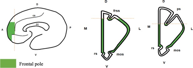
Boundaries of the frontal pole.
From left to right: sagittal view, coronal view for great apes and humans, coronal view for monkeys. Frontal pole is in green. Abbreviations: cs: cingulate sulcus; cc: corpus callosum; rs: rostral sulcus; mos: medial-orbital sulcus; frss: superior frontal sulcus; ps: principal sulcus; D: dorsal; V: ventral; M: medial; L: lateral; A: anterior; P: posterior.

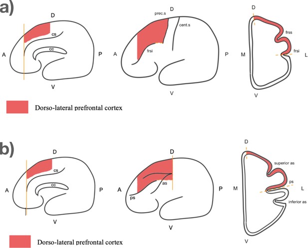
Boundaries of the dorso-lateral prefrontal cortex.
(a) For great apes and humans. From left to right: sagittal view, external view, coronal view. Abbreviations: cs: cingulate sulcus; cc: corpsus callosum; frsi: frontal inferior sulcus; frss: frontal superior sulcus; cent.s: central sulcus; prec.s: precentral sulcus; A: anterior: P: posterior; D: dorsal; V: ventral; L: lateral; M: medial. (b) For monkeys. From left to right: sagittal view, external view, coronal view. Abbreviations: cs: cingulate sulcus; cc: corpsus callosum; ps: principal sulcus; as: arcuate sulcus; A: anterior: P: posterior; D: dorsal; V: ventral; L: lateral; M: medial.

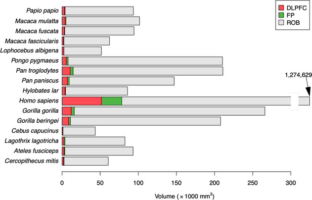
Average values of the three regions of interest.
Each line provides the cumulated volumes of the dorso-lateral prefrontal cortex (DLPFC, green), the frontal pole (FP, gray), and the rest of the brain (ROB, blue), such that the size of each bar represents the whole brain volume. Note: for Homo sapiens, the bar has been truncated, since its value was out of scale with the other species.
Tables
Estimated coefficients of socio-ecological variables for the whole brain volume.
| Predictor | Beta (estimate) | Beta (std. error) | Standardized beta | t-Value | p- Value |
|---|---|---|---|---|---|
| Intercept | 4.26 | 0.24 | 17.8 | 0 | |
| Body mass (log) | 0.47 | 0.15 | 0.71 | 3.10 | 0.009 |
| Daily traveled distance | 0.05 | 0.01 | 0.42 | 4.08 | 0.002 |
| Population density | 0.007 | 0.003 | 0.35 | 2.35 | 0.036 |
Estimated coefficients of socio-ecological variables for the frontal pole volume.
| Predictor | Beta (estimate) | Beta (std. error) | Standardized beta | t-Value | p.-Value |
|---|---|---|---|---|---|
| Intercept | 1.87 | 0.37 | 5.08 | 0 | |
| Body mass (log) | 0.69 | 0.23 | 0.66 | 2.96 | 0.012 |
| Daily traveled distance | 0.07 | 0.02 | 0.36 | 3.62 | 0.004 |
| Population density | 0.011 | 0.004 | 0.38 | 2.62 | 0.022 |
Estimated coefficients of socio-ecological variables for the dorso-lateral prefrontal cortex (DLPFC) volume.
| Predictor | Beta (estimate) | Beta (std. error) | Standardized beta | t-Value | p-Value |
|---|---|---|---|---|---|
| Intercept | 2.78 | 0.28 | 9.99 | 0 | |
| Body mass (log) | 0.47 | 0.18 | 0.62 | 2.67 | 0.021 |
| Daily traveled distance | 0.047 | 0.014 | 0.35 | 3.3 | 0.006 |
| Population density | 0.006 | 0.003 | 0.30 | 2.01 | 0.067 |
Additional files
-
Supplementary file 1
Table of AIC values for each predictor of the best model, for each of the brain regions (‘response’ of the model).
AIC values have been computed for a regression model without (OLS) and with (phylogenetic generalized least squares [PGLS]) phylogenetic correlation. The smallest value for each brain region (response) is in bold.
- https://cdn.elifesciences.org/articles/87780/elife-87780-supp1-v1.docx
-
Supplementary file 2
Standardized coefficients.
This table indicates the values of the normalized coefficients for each of the brain region and each of the variables of the regression models.
- https://cdn.elifesciences.org/articles/87780/elife-87780-supp2-v1.docx
-
Supplementary file 3
Details of the leave-one-out analysis for the whole brain.
Each of the three panels corresponds to one of the variables of the model, and shows the value (colored dots) of the estimated coefficient for that variable after the data of the corresponding species has been removed from the analysis. The color code is indicated on the figure, below Pop_d panel. As a reminder, we added the values of these estimated coefficients (together with t and p statistics) when all species are included. The values of these ‘original’ coefficients (i.e. when all species are included) are indicated by a vertical dotted line on the panel of each of these variables. Body: body weight; DTD: daily traveled distance; Pop_d: population density.
- https://cdn.elifesciences.org/articles/87780/elife-87780-supp3-v1.pdf
-
Supplementary file 4
Alternative analysis with less conservative evaluation of the frontal pole (FP) volume.
For 10 species (i.e. the monkeys species), the volume of FP was re-assessed as described in the text, because the delimitation of the FP could be considered from a different perspective. This procedure was not necessary for great apes and humans, because in those species the delimitation of FP was easier. In short, we used a conservative measure of the FP in monkeys, which did not include the dorsal part of the anterior prefrontal cortex. Indeed, even anatomo-functional studies suggest that the the FP could extend more dorsally in macaques, that dorsal region also includes Brodmann area 9 (BA 9), which is usually associated with the DLPFC (Sallet et al., 2013; Petrides, 2005. Petrides et al., 2012). But since that dorsal area could also be associated with the FP, we conducted a new analysis where the FP volume did include that dorsal area. Fig SF 4.1. Relation between conservative and inclusive measures of the FP volume Table SF 4.2: Model comparison data for the inclusive measure of the FP. Each line corresponds to a model tested to account for the variability of FP volumes across species. Each model is defined as a set of predictors. We provide the AIC of each model using both OLS and PGLS regression methods. For each method, the AIC value of the best model (smallest AIC value) is indicated in bold. Table SI 4.3. Parameter estimate for the best model according to OLS. The table provides the mean beta estimate, its standard error (SE), as well as the corresponding t statistic and p-value estimate for each of the parameters of the best model based on OLS approach (i.e. AIC = 10.22). Table S4.4. Parameter estimate for the best model according to PGLS. The table provides the mean beta estimate, its SE, as well as the corresponding t statistic and p value estimate for each of the parameters of the best model based on PGLS approach (i.e. AIC = 10.25).
- https://cdn.elifesciences.org/articles/87780/elife-87780-supp4-v1.docx
-
Supplementary file 5
Details of the leave-one-out analysis for the frontal pole (FP).
Each of the three panels corresponds to one of the variables of the model, and shows the value (colored dots) of the estimated coefficient for that variable after the data of the corresponding species has been removed from the analysis. The color code is indicated on the figure, below Pop_d panel. As a reminder, we added the values of these estimated coefficients (together with t and p statistics) when all species are included. The values of these ‘original’ coefficients (i.e. when all species are included) are indicated by a vertical dotted line on the panel of each of these variables. Body: body weight; DTD: daily traveled distance; Pop_d: population density.
- https://cdn.elifesciences.org/articles/87780/elife-87780-supp5-v1.pdf
-
Supplementary file 6
Details of the leave-one-out analysis for the dorso-lateral prefrontal cortex (DLPFC).
Each of the three panels corresponds to one of the variables of the model, and shows the value (colored dots) of the estimated coefficient for that variable after the data of the corresponding species has been removed from the analysis. The color code is indicated on the figure, below Pop_d panel. As a reminder, we added the values of these estimated coefficients (together with t and p statistics) when all species are included. The values of these ‘original’ coefficients (i.e. when all species are included) are indicated by a vertical dotted line on the panel of each of these variables. Body: body weight; DTD: daily traveled distance; Pop_d: population density.
- https://cdn.elifesciences.org/articles/87780/elife-87780-supp6-v1.pdf
-
Supplementary file 7
Relation across socio-ecological variables.
There are six continuous and five categorical variables. Table SF7.1. Shows pairwise correlations for all pairs of continuous variables (Pearson correlation coefficients below the diagonal; p-values above the diagonal). If we consider a Bonferroni correction for these tests, the critical p-value becomes 0.05/3=0.003. Legends: Body for body mass; QI for dietary quality index; DTD for daily traveled distance; Gp for group size; Pop_d for population density; weaning for ratio weaning period/lifespan. Fig SF 7.2. Shows Pairwise plots of correlations across these continuous socio-ecological variables. Table SF 7.3. Contingency table of the two correlated categorical variables: social system and mating system. Among the five categorical variables, only one pair was statistically significant (Fisher test, p=0.0009): social system and mating system. These two variables are actually mostly redundant as shown by their contingency table. Fig SF 7.4. Relations between continuous vs categorical variables. When looking at the relationships between a continuous and a categorical variables, social system appeared as related to most continuous variables, especially body mass and weaning. Table SF 7.5. Quantification of the relation between continuous vs categorical variables. We performed an ANOVA on these 30 pairs with the continuous variable as response. Setting the significance threshold at 0.05/30=0.0017, only one fit was statistically significant: social system on body mass. If the response (continuous variable) was log-transformed, only one analysis was significant: social system on group size.
- https://cdn.elifesciences.org/articles/87780/elife-87780-supp7-v1.docx
-
Supplementary file 8
Construction of the socio-ecological database.
Table SF 8.1. Socio-ecological variables. This table indicates the socio-ecological variables of interest for each of the species. BM: body mass (kg); DQI: dietary quality index; TU: tool use (yes/no); DTD: daily traveled distance (km); GS: group size; Pop D: population density (ind/km2); Soc. System: social system; MG: mate guarding (yes/no); Seas. B: seasonal breading (yes/no); Mating syst: Mating system. WL: ratio weaning period/lifespan. Table SF 8.2. References socio-ecological variables. This table shows the references used to calculate the values of each socio-ecological variable of each species. Only names and dates of publication are provided in the table, but detailed references are provided in the list below.
- https://cdn.elifesciences.org/articles/87780/elife-87780-supp8-v1.docx
-
MDAR checklist
- https://cdn.elifesciences.org/articles/87780/elife-87780-mdarchecklist1-v1.pdf


