Streamlining segmentation of cryo-electron tomography datasets with Ais
- Department of Cell and Chemical Biology, Leiden University Medical Center, Netherlands
- Institute of Science and Technology Austria (ISTA), Austria
- School of Biochemistry, University of Bristol, United Kingdom
Figures
Figure 1 with 4 supplements

An overview of the user interface and functionalities.
The various panels represent sequential stages in the Ais processing workflow, including annotation (A), testing convolutional neural networks (CNNs) (B), and visualizing segmentation (C). These images (A–C) are unedited screenshots of the software. (A) The interface for annotation of datasets. In this example, a tomographic slice has been annotated with various features – a detailed explanation follows in Figure 5. (B) After annotation, multiple neural networks are set up and trained on the aforementioned annotations. The resulting models can then be used to segment the various distinct features. In this example, double-membrane vesicles (double membrane vesicles DMVs, red), single membranes (blue), ribosomes (magenta), intermediate filaments (orange), mitochondrial granules (yellow), and molecular pores in the DMVs (lime) are segmented. (C) After training or downloading the required models and exporting segmented volumes, the resulting segmentations are immediately available within the software for 3d rendering and inspection. (D) The repository at aiscryoet.org facilitates the sharing and reuse of trained models. After validation, submitted models can be freely downloaded by anyone. (E) Additional information, such as the pixel size and the filtering applied to the training data, is displayed alongside all entries in the repository, in order to help a user identify whether a model is suited to segment their datasets.
Figure 1—figure supplement 1
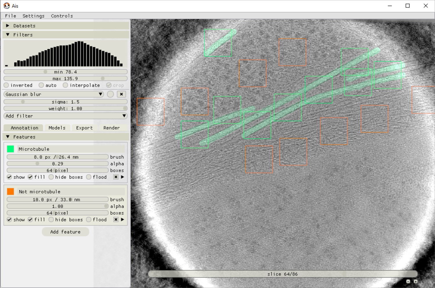
Ais annotation interface.
The image shows an example of microtubules (green) being annotated and positive (green boxes) and negative (orange boxes) training boxes being placed. Neural networks in Ais operate on square input images (here 64 × 64 pixels), and the training data thus consists of square pairs of images, with the grayscale data in a placed box as the training input and the user-drawn annotations in that same box as the training output.
Figure 1—figure supplement 2
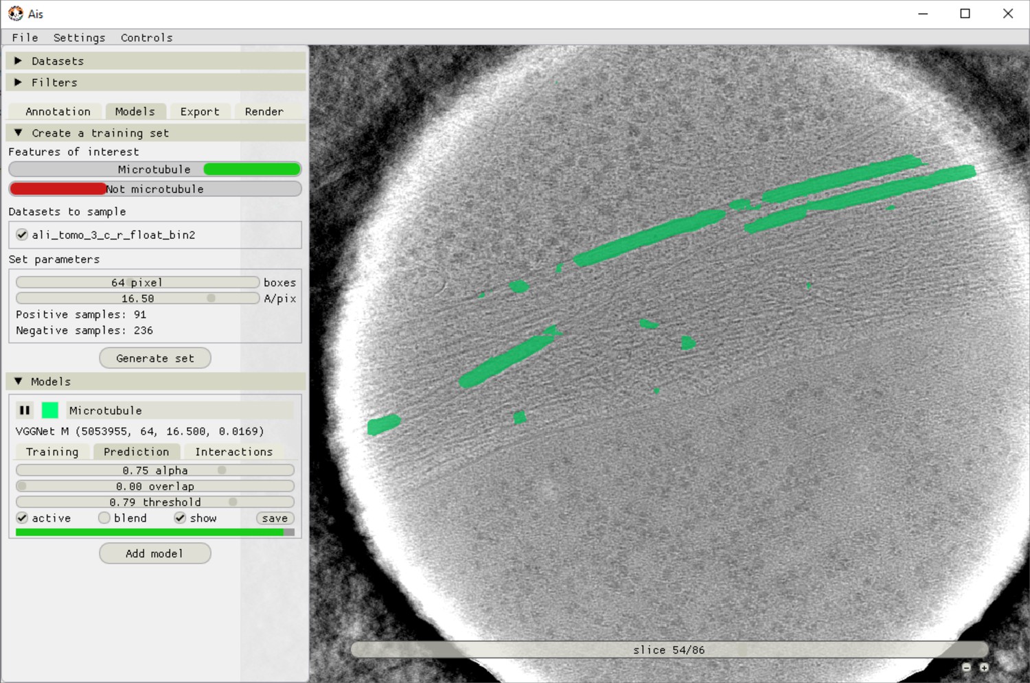
Ais training and model testing interface.
After annotation and boxing, different training datasets can be exported by selecting which annotations to use as positives and which as negatives. In this example, the ‘Microtubule’ annotations are included as a positive feature, meaning both the input grayscale and output annotation are sampled. The feature ‘Not microtubule’ is included as a negative feature, meaning input grayscale is sampled and the corresponding output annotations are all zeroes. Using separate positive and negative annotation classes is not necessary (including unlabelled boxes in the ‘Microtubule’ annotations has the same effect as using a negative class), but can be convenient.
Figure 1—figure supplement 3
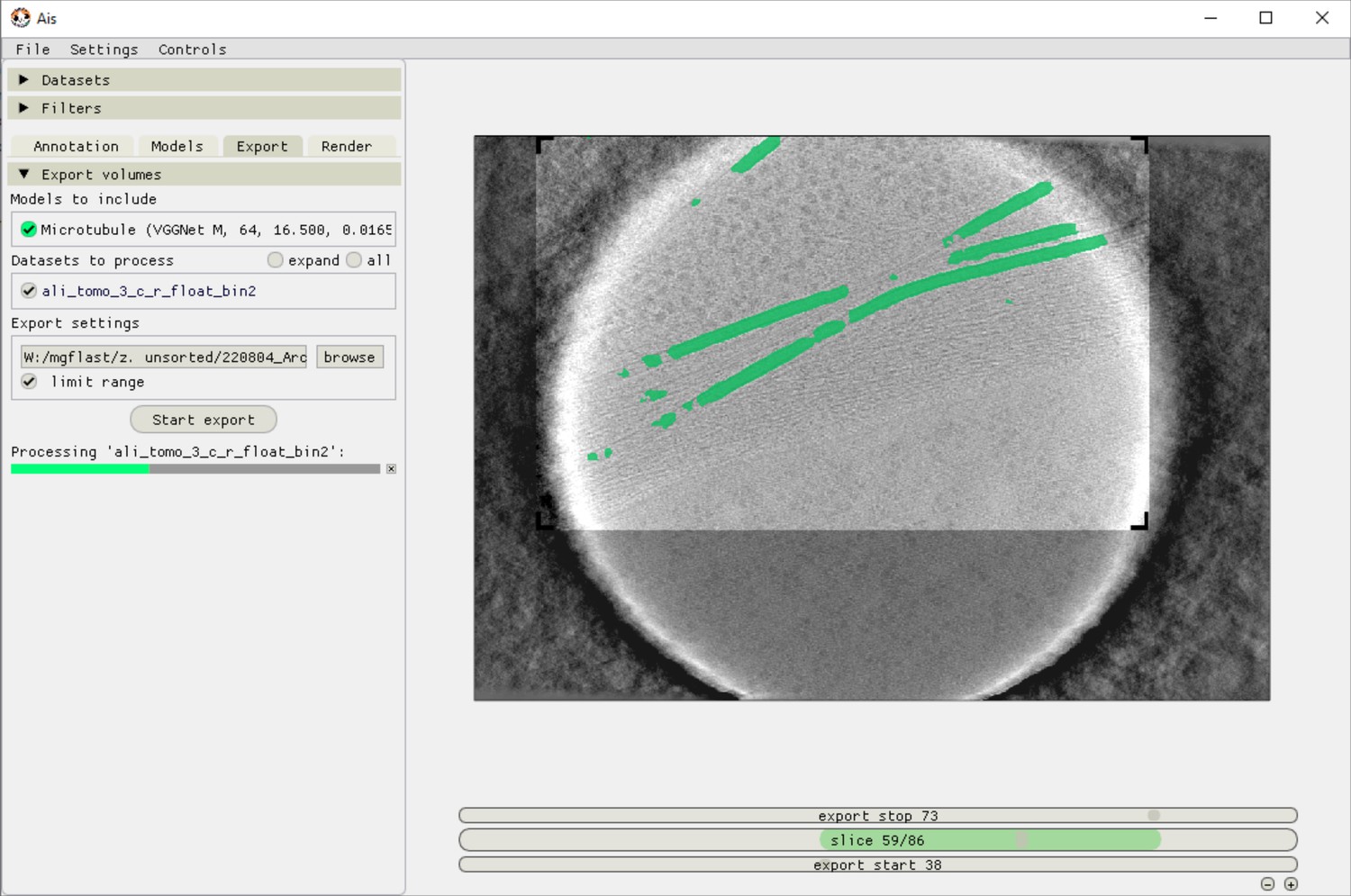
Ais volume exporting interface.
After preparing a suitable network for segmentation, users can apply this network to any tomogram in the ‘Export’ tab. Applying one network to one volume typically takes around 1 min, although depending on the available hardware and the size of the volume. In this example, the network is only applied to a selected area of interest in order to save time processing.
Figure 1—figure supplement 4

Ais 3D rendering interface.
After exporting segmented volumes, these segmentations are immediately available for 3D rendering in the ‘Render’ tab. Volumes are rendered as isosurface meshes, and can also be saved as such (as.obj files), or opened in other rendering software such as Blender or ChimeraX11.
Figure 2 with 1 supplement

A comparison of different neural networks for tomogram segmentation.
(A) A representative example of the manual segmentation used to prepare training datasets. Membranes are annotated in red, carbon film in bright white, and antibody platforms in green. For the antibody training set, we used annotations prepared in multiple slices of the same tomogram, but for the carbon and membrane training set the slice shown here comprised all the training data. (B) A tomographic slice from a different tomogram that contains the same features of interest, also showing membrane-bound antibodies with elevated Fc platforms that are adjacent to carbon (red arrowheads). (C) Results of segmentation of membranes (top; red), carbon (middle; white), and antibody platforms (bottom; green), with the six different neural networks.
Figure 2—figure supplement 1
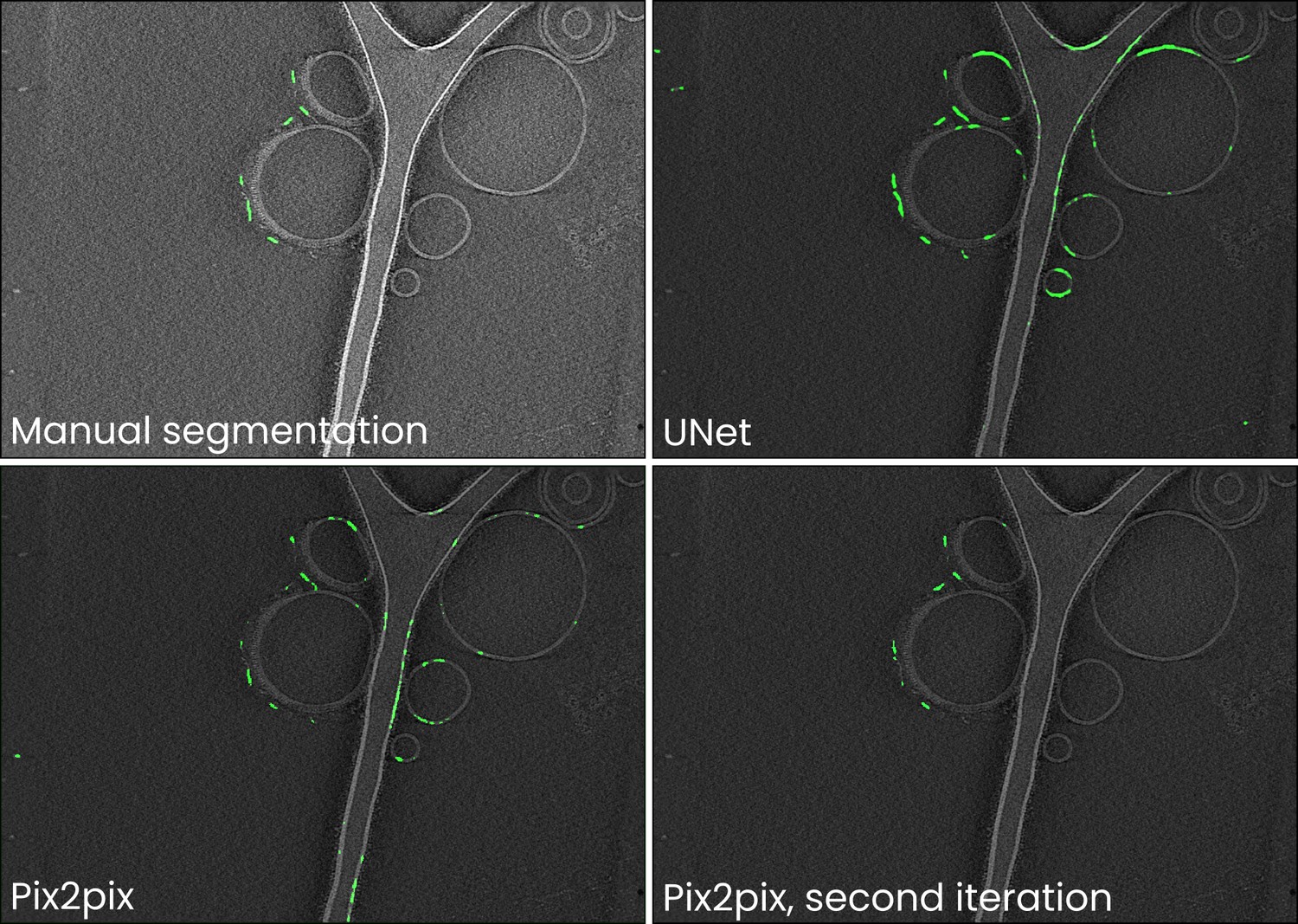
Comparison of manual annotations and UNet, Pix2pix, and improved Pix2pix antibody platform segmentations for the data in Figure 2.
Training neural networks can often be an iterative process: an initial training dataset is compiled, a model trained, and the resulting segmentations are likely to contain readily identifiable false negatives (i.e. parts of antibody platforms not annotated by a model) and positives (e.g. membranes segmented as antibody platforms). To improve the model, it is then useful to perform a second iteration of annotating boxes for use in training and then training the model anew. In Ais, this is facilitated by being able to switch back and forth between the ‘annotation’ and ‘models’ tabs, and by being able to quickly test models on and annotate new boxes in many different datasets. In this example, we initially trained Pix2pix on the same training dataset as used for the other networks discussed in Figure 2 and Table 1 in the main text. Although the loss of the UNet network was the lowest, we found that in comparison to most other networks the output of the Pix2pix model contained fewer false positive predictions (e.g. compare the segmentations of the liposome membranes). Since Pix2pix is a large model, it is likely to benefit the most from further training on an expanded training dataset. We thus included additional samples in the training dataset and trained a new instance of a Pix2pix model for 50 epochs. The resulting model produced segmentations that were much closer to the manual annotations. Further information and tips for preparing useful models are also discussed in the video tutorials, available at youtube.com/@scNodes.
Figure 3

Model interactions can significantly increase segmentation accuracy.
(A) An overview of the settings available in the ‘Models’ menu in Ais. Three models: (1) ‘membrane’ (red), (2) ‘carbon’ (white), and (3) ‘antibody platforms’ (green) are active, with each showing a different section of the model settings: the training menu (1), prediction parameters (2), and the interactions menu (3). (B) A section of a tomographic slice is segmented by two models, carbon (white; parent model) and membrane (red; child model), with the membrane model showing a clear false positive prediction on an edge of the carbon film (panel ‘without interactions’). By configuring an avoidance interaction between the membrane model that is conditional upon the carbon model’s prediction, this false positive is avoided (panel ‘with interactions’). (C) By setting up multiple model interactions, inaccurate predictions by the ‘antibody platforms’ model are suppressed. In this example, the membrane model avoids carbon while the antibody model is set to colocalize with the membrane model. (D) 3D renders (see Methods) of the same dataset as used in Figure 2 processed three ways: without any interactions (left), using model competition only (middle), or by using model competition as well as multiple model interactions (right).
Figure 4 with 3 supplements

Automated particle picking for sub-tomogram averaging of antibody complexes.
(A) Manually prepared annotations used to train a neural network to recognize antibody platforms (top) or antibody-C1 complexes (bottom). (B) Segmentation results as visualized within the software. Membranes (red) and carbon support film (white) were used to condition the antibody (green) and antibody-C1 complex (yellow) predictions using model interactions. (C) 3D representations of the segmented volumes rendered in Ais. (D) Tomographic slices showing particles picked automatically based on the segmented volume shown in panel c. (E) Subtomogram averaging result of the 2499 automatically picked antibody platforms. (F) Subtomogram averaging result obtained with the 602 automatically picked antibody-C1 complexes. The quadrants in panels e and f show orthogonal slices of the reconstructed density maps and a 3D isosurface model (the latter rendered in ChimeraX [Goddard et al., 2018]).
Figure 4—figure supplement 1
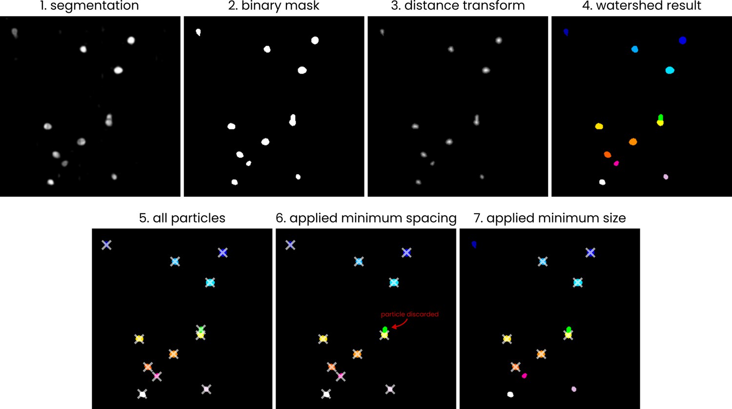
A visual (2D) representation of the processing steps employed in the automated picking process.
The steps employed in the process of converting a segmented.mrc volume to a list of particle coordinates. The example is shown in 2D; the actual picking process is performed in 3D. (1) The input segmentation (values 0–255), (2) a binary mask, generated by thresholding the input image at a value of 127, (3) the distance transform of the binary mask, (4) groups of pixels, labelled using a watershed algorithm (skimage.segmentation.watershed) with local maxima in the distance transform output used as sources, (5) centroid coordinates (marked by crosses) of the pixel groups, (6) example of removing particles by applying a minimum spacing, (7) example of removing particles by specifying a minimum particle size.
Figure 4—figure supplement 2
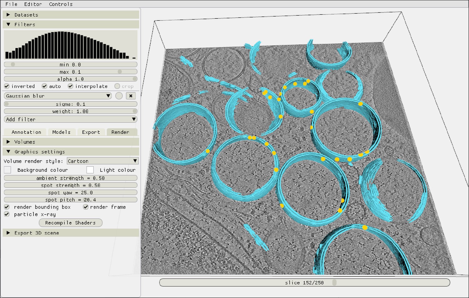
Inspecting the autopicking results in the Ais renderer.
After picking particles, the resulting localizations are immediately available for inspection in the renderer. In this example, yellow markers indicate the coordinates of molecular pores, picked in a tomogram from the dataset by Wolff et al., 2020 (see main text Figure 5).
Figure 4—figure supplement 3
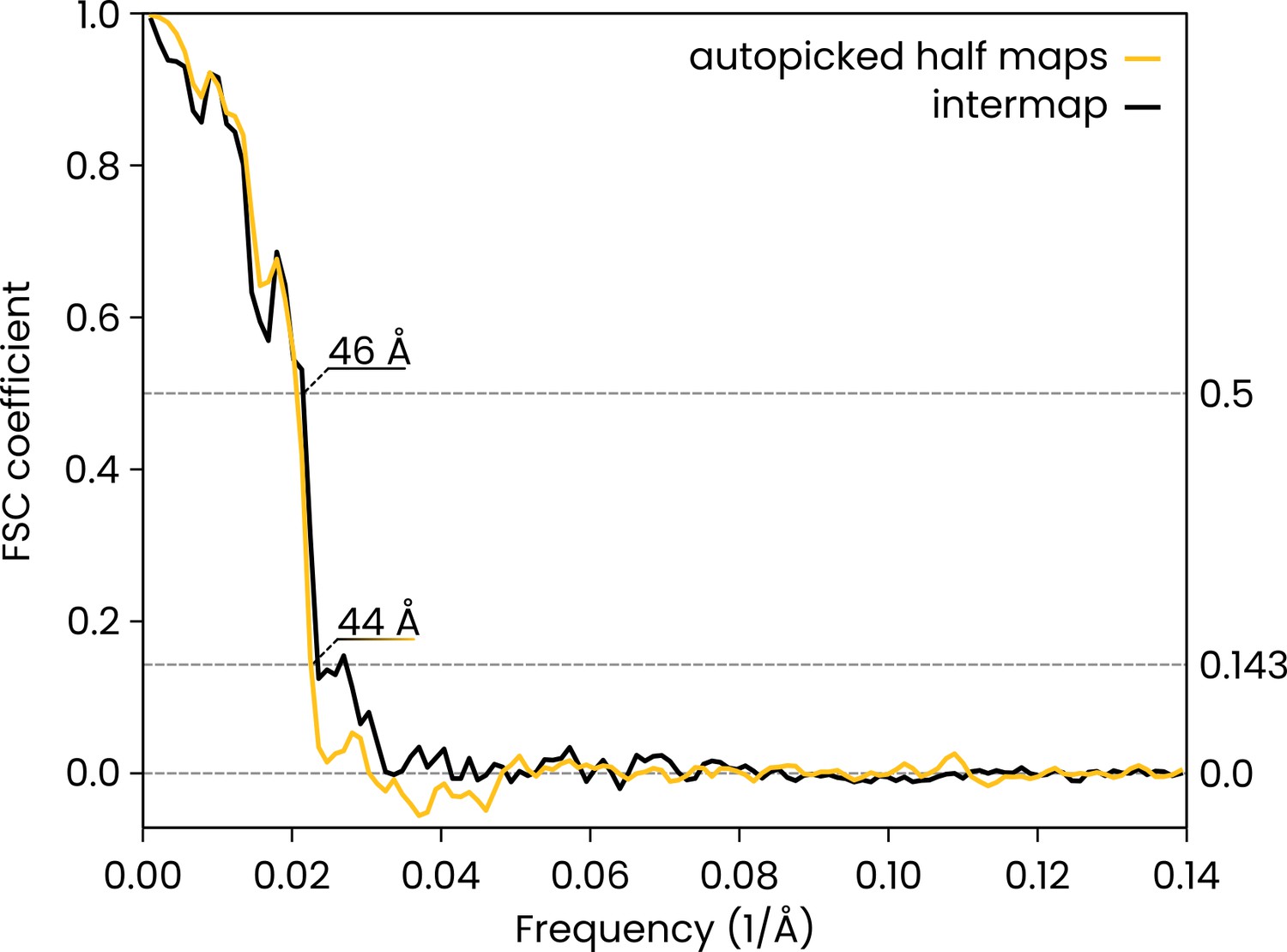
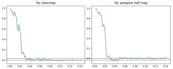
Comparison of the automatically picked C1-IgG3 complex reconstruction versus the original reconstruction in Abendstein et al., 2023.
The FSC curve for the two half maps of the automatically-picked C1-IgG3 complex reconstruction gives a resolution of 44 Å at the FSC = 0.143 (yellow, 'auto picked half maps'). In the original publication (Abendstein et al., 2023) various resolutions are reported for different maps that were obtained by focused refinement on different parts of the complex. In the current report, we did not apply further refinement steps beyond the initial even/odd reconstructions on the entire complex that the above FSC curve is based on. The value of 44 Å must thus be compared to the corresponding initial reconstruction in the original report (in Abendstein et al., 2023, their Supplementary Fig. 10c, map #1) which was reported at FSC = 0.143 with the same resolution of 44 Å. A comparison between the full maps (black FSC curve, 'intermap') at FSC coefficient 0.5 gives a value of 46 Å for the resolution, thus indicating that the two independent reconstructions did indeed converge on the same structure.
Figure 5 with 2 supplements

Segmentations of complex in situ tomograms.
(A) A segmentation of seven distinct features observed in the base of C. reinhardtii cilia (van den Hoek et al., 2022, EMPIAR-11078, tomogram 12): membranes (gray), ribosomes (magenta), microtubule doublets (green) and axial microtubules (green), non-microtubular filaments within the cilium (blue), inter-flagellar transport trains (yellow), and glycocalyx (orange). Inset: a perpendicular view of the axis of the cilium. The arrows in the adjacent panel indicate these structures in a tomographic slice. (B) A segmentation of six features observed in and around mitochondria in a mouse neuron with Huntington’s disease phenotype (Wu et al., 2023) (EMD-29207): membranes (gray), mitochondrial granules (yellow), membranes of the mitochondrial cristae (red), microtubules (green), actin (turquoise), and ribosomes (magenta). (C) Left: a segmentation of ten different cellular components found in tomograms of coronavirus-infected mammalian cells (Wolff et al., 2020): double-membrane vesicles (double membrane vesicles DMVs, light red), single membranes (gray), viral nucleocapsid proteins (red), viral pores in the DMVs (blue), nucleic acids in the DMVs (pink), microtubules (green), actin (cyan), intermediate filaments (orange), ribosomes (magenta), and mitochondrial granules (yellow). Right: a representative slice, with examples of each of the features (except the mitochondrial granules) indicated by arrows of the corresponding colour.
Figure 5—figure supplement 1
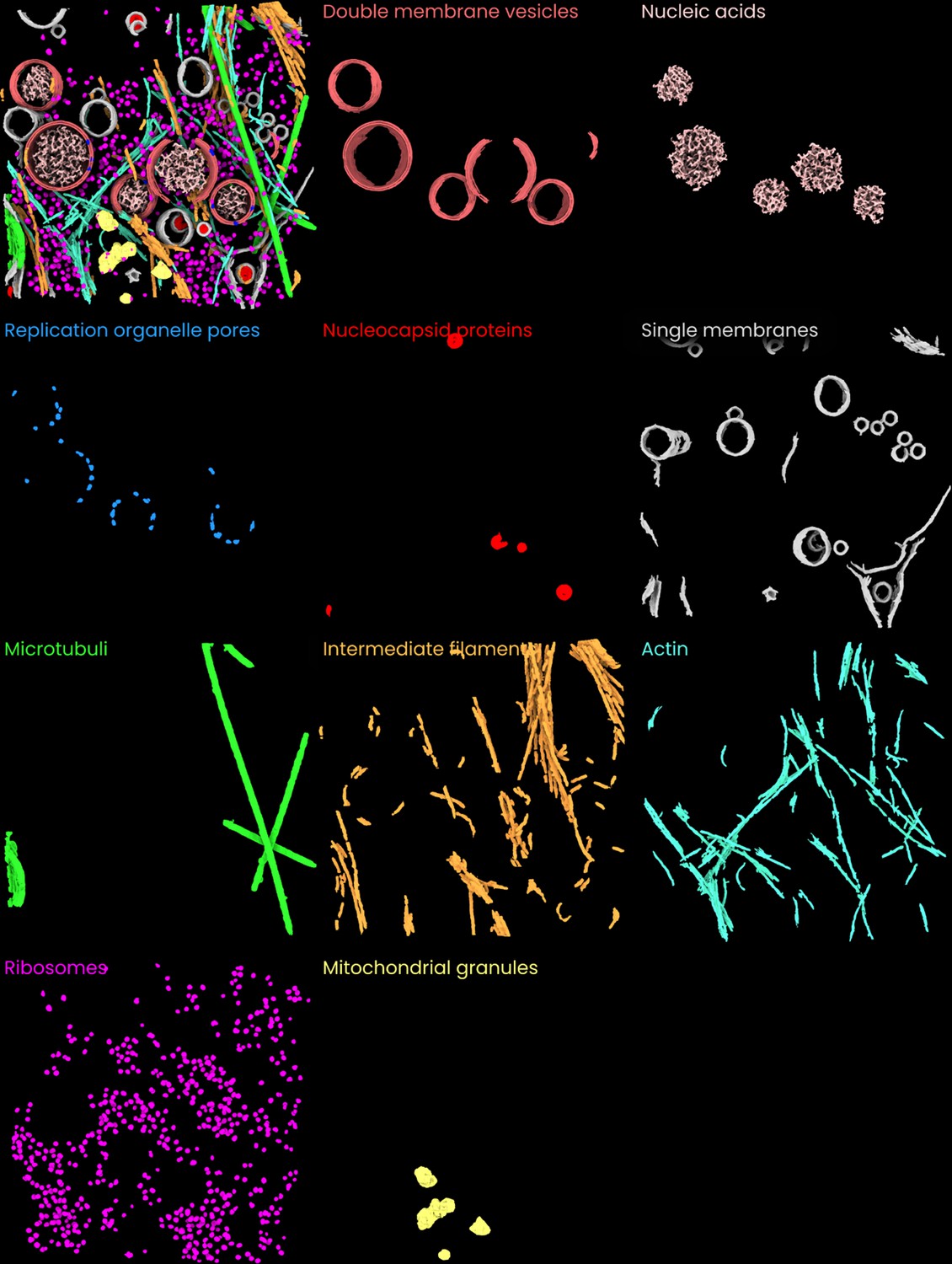
Individual images of the ten features segmented in the coronavirus-infected mammalian cells dataset (Wolff et al., 2020, Science).
A side-by-side overview of the 10 segmented features in the coronavirus-infected mammalian cells dataset.
Figure 5—figure supplement 2
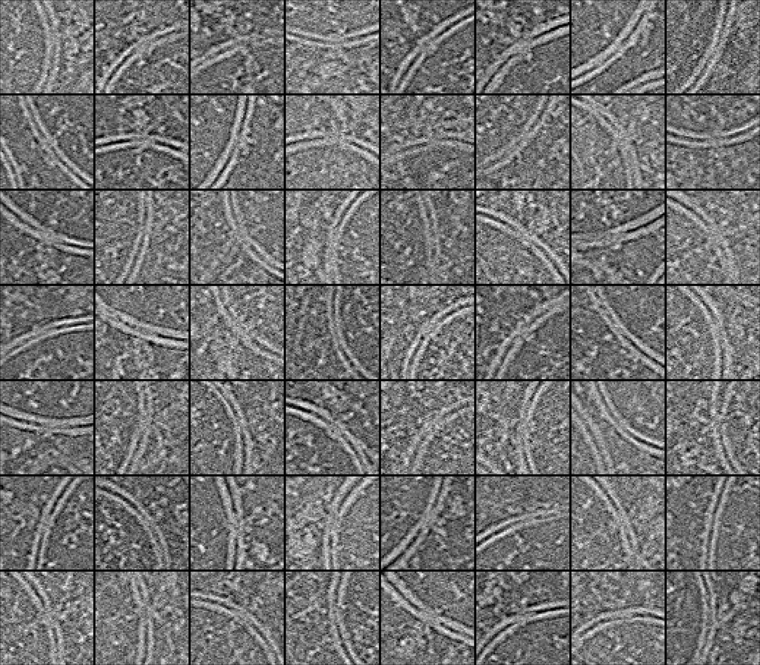
A collage of automatically picked molecular pores in the double membrane vesicles.
As with the C1-IgG3 complexes and IgG3 platforms (main Figures 3 and 4), the segmentations of the molecular pores in the coronavirus replication organelle (main Figure 5) can be used to automatically pick particles. In the above image, tomographic slices are shown that were cropped at the location of 56 particles (picked in two tomograms). Although it can be difficult to tell at the single particle level whether an image contains the exact structure of interest, the images are all centered on sections of double-membrane vesicles and many show additional density between the membranes as well as at the outside (convex side) of the vesicle, characteristic of the molecular pore. The accuracy of picking and the quality of the resulting particle datasets are dependent on the quality of the original segmentations and on the parameters used in picking. Converting a 3D grayscale volume to a list of coordinates requires a number of parameters to be specified (in Ais, but also in many other programs). First, a threshold value is used to convert from grayscale to a binary volume. Contiguous regions of nonzero voxels in the volumes are then considered ‘particles,’ and various metrics can be used to determine whether particles are included in the final list of coordinates. Example are the particle volume, integrated prediction value for the voxels included in the particle’s volume, or a minimum particle spacing. In Ais, users can specify the first and the latter (we experimented with using the second metric as well, but found it very similar but less intuitive than the metric of particle volume, so we did not include it). The threshold values chosen for these metrics and for the conversion of the grayscale volume to a binary one thus define what is ‘dust.’ In practice, choosing these values entails a trade-off between the number of particles, and the ‘quality’ of the selected set of particles. Low thresholds yield a large number of particles, which can introduce the need to perform classification during reconstruction by subtomogram averaging. High thresholds yield fewer particles, but the resulting selection may be more uniform, and their images of higher quality. In practice, it is advisable to test different thresholds and to inspect the resulting particle datasets, in order to ensure that (i) good particles are not being excluded, and (ii) large numbers of bad particles (e.g. densities that correspond to structures other than the structure of interest) are not being included. As with manually picked particle sets, classification is likely required to curate the selection of particles.
Appendix 1—figure 1

Uploading a model to the model repository via aiscryoet.org/upload.
Author response image 1
Author response image 2

Tables
Table 1
Comparison of some of the default models available in Ais.
aThe computational cost is only roughly proportional to the number of model parameters, which is reported in the software. The specifics of the network architecture affect the processing speed more significantly. bTime required to process one 511 × 720 pixel-sized tomographic slice. cThese columns list the loss values after training, calculated as the binary cross-entropy (bce) between the prediction and original annotation. The loss is a (rough) metric of how well a trained network performs (see Methods). dUnlike the other architectures, Pix2pix is not trained to minimize the bce loss but uses a different loss function instead. The bce loss values shown here were computed after training and may not be entirely comparable.
| Architecture | Parameters | Training timea | Processing timea, b | Membranec | Carbonc | Antibodyc |
|---|---|---|---|---|---|---|
| EMAN2 | 378,081 | 38 s | 50 ms | 0.044 | .072 | .010 |
| InceptionNet | 550,529 | 462 s | 295 ms | 0.046 | .120 | .008 |
| UNet | 922,881 | 132 s | 110 ms | 0.013 | .007 | .001 |
| VGGNet | 1,493,059 | 91 s | 85 ms | 0.011 | .125 | .013 |
| ResNet | 4,887,265 | 1533 s | 980 ms | 0.047 | .060 | .014 |
| Pix2pixd | 29,249,409 | 793 s | 225 ms | 0.050d | .129d | .016d |
Additional files
Download links
A two-part list of links to download the article, or parts of the article, in various formats.
Downloads (link to download the article as PDF)
Open citations (links to open the citations from this article in various online reference manager services)
Cite this article (links to download the citations from this article in formats compatible with various reference manager tools)
Streamlining segmentation of cryo-electron tomography datasets with Ais
eLife 13:RP98552.
https://doi.org/10.7554/eLife.98552.3


