Adaptability of non-genetic diversity in bacterial chemotaxis
- Yale University, United States
Figures
Figure 1

From proteins to fitness.
(A) The cell receives extracellular ligand signals through transmembrane receptors. Changes in signal are rapidly communicated to the flagellar motors through the kinase CheA and response regulator CheY. CheZ opposes the kinase activity of CheA. At a slower timescale, the activity of the receptor complex physiologically adapts to its steady-state activity through the antagonistic actions of CheR and CheB. (B) Cartoon diagram of the response of the system to transient step-stimulus and definition of the key phenotypic parameters of the system. Without stimulation, the system has a steady-state clockwise bias, or fraction of time spent with motors in the clockwise state that results in tumbling. Upon stimulus with a step, CheY activity and therefore clockwise bias drops and the cell starts running more, then slowly adapts back to the steady-state with a characteristic timescale (adaptation time). The steady-state clockwise bias and adaptation time are tuned by the concentrations of proteins in (A). (C) Cells explore their environment by alternating between straight runs and direction-changing tumbles. When cells sense that they are traveling up a concentration gradient, they suppress tumbles to increase run length. Precisely how a cell navigates a gradient depends on its phenotypic parameters in (B). (D) From a single genotype, noise in gene expression leads to a distribution of proteins expression levels (blue shaded contours in protein space; left); network design determines how proteins quantities map onto phenotypic parameters (middle left); the performance of all possible phenotypic parameter values across environments will determine the outer boundary of performance space (middle right); selection bestows a fitness reward based on performance and will reshape the performance front into the Pareto front, which, for optimal fitness, the population distribution should be constrained to (right).
Figure 2 with 8 supplements

Performance of chemotactic phenotypes depends on environmental conditions.
(A) Cartoon diagram (not to scale) of the foraging challenge: cells navigating a 3-D time-varying gradient created by diffusion of a small spherical drop of nutrient 100 µm in diameter with diffusion coefficient of 550 µm2/s and methyl-aspartate concentration of 100 mM. Inset: radial profile of the attractant concentration over time. (B) Average nutrient collected by each phenotype (combination of clockwise bias and adaptation time) in environment in A over 8000 replicates per phenotype. Because we are investigating optimal phenotypes and CheY-P dynamic range does alter the results as long as it is sufficiently high (Figure 2—figure supplement 7), results shown here use YTot = 13,149 mol./cell. Clockwise bias and adaptation time were sample in log-spaced bins. Cells start near to the source (0.2 mm from its center), and are allowed to swim for 13 min while accumulating a small fraction of the nutrient they sense. (C). Same as B except that cells start farther away from the source (1 mm from its center) and 14,000 replicates per phenotype were used. (D–F) Similar to (A–C) but the environment consists of a colonization challenge: diffusion of ligand out of a spherical non-depleting source representing a colonization site; source methyl-aspartate concentration was 10 mM. Rather than nutrient collection, performance (E and F) was quantified as the reciprocal of the arrival time at the source averaged over all replicates (9000 and 36,000 for E and F respectively) with a maximum time allotted of 15 min.
Figure 2—figure supplement 1
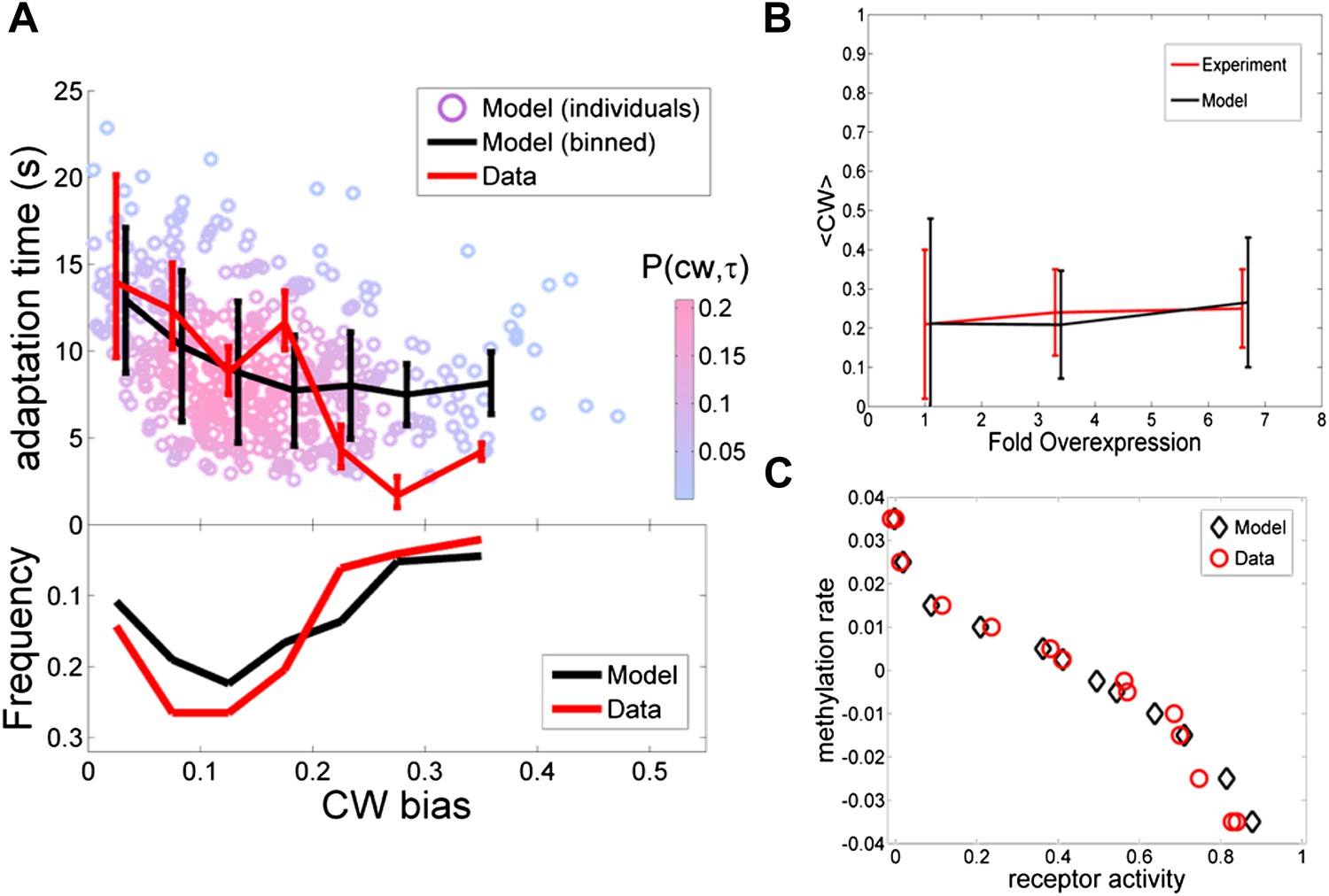
Comparing the model to single cell and population averaged measurements.
The same set of model parameter values is used for all the plots. (A) Adaptation time and motor clockwise (CW) bias. Bottom: normalized histogram of motor clockwise bias in the population. Top: The mean and standard deviation of adaptation time in each bin of CW bias. Red lines: experimental data from ref. 4. Black lines: model. Circles: Individual cells from the model. Color: probability density. (B) Population-averaged CW bias as a function of fold changes in mean expression level of all pathway proteins following ref. 7. Red: data from ref. 7. Black: model. (C) Population-averaged methylation rate as a function of population-averaged receptor activity obtained by exposing cells to exponential ramps of methyl-aspartate as described in ref. 42. Red circles: data from ref. 42. Black: simulation of model.
Figure 2—figure supplement 2
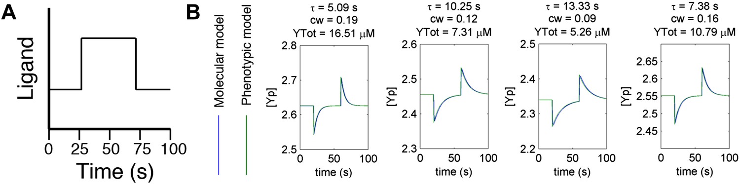
Agreement between protein model and parametric dynamics model.
(A) Cartoon of step function of ligand delivered to immobilized cells in simulation to test response dynamics. (B) Direct comparison of response of molecular model (blue) and phenotypic model (green) with the same parameters to stimulus of the form in A illustrating close agreement.
Figure 2—figure supplement 3
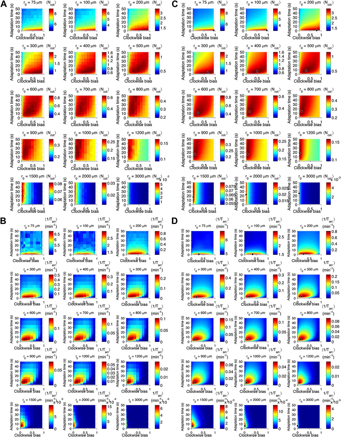
Performance as a function of distance to source.
(A) Cells with various phenotypes were challenged to forage a source presented at varying distances, r0 from 75 μm to 3 mm. Between 6000 and 30,000 replicates were simulated for each phenotype. : the average nutrient collected by all replicates of a given phenotype in μmol. (B) Same as A but for a colonization challenge; : the average reciprocal-of-arrival-time of all of the replicates of a given phenotype in min−1. (C) Data in A smoothed with a Gaussian filter and resampled on a higher resolution grid of phenotypic parameters. Diamond: phenotype with highest performance. (D) Same as C but with the data in (B).
Figure 2—figure supplement 4
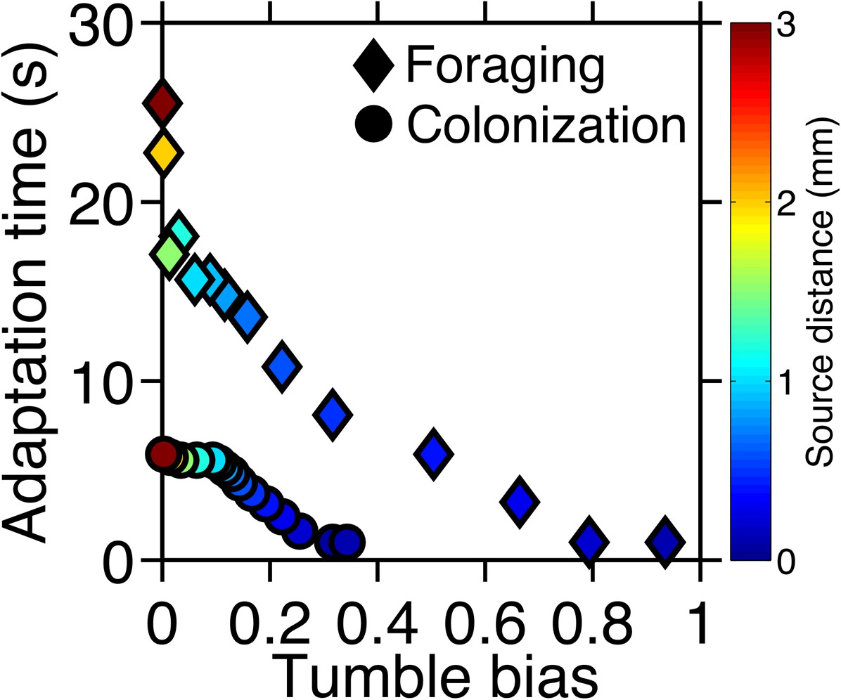
Optimal phenotypes as a function of source distance.
For each source distance and each task, the phenotype with highest performance was identified as shown in Figure 2—figure supplement 3. The clockwise bias and adaptation time of these phenotypes are shown with the marker color corresponding to the distance to the source. Diamonds: foraging case. Circles: colonization case.
Figure 2—figure supplement 5
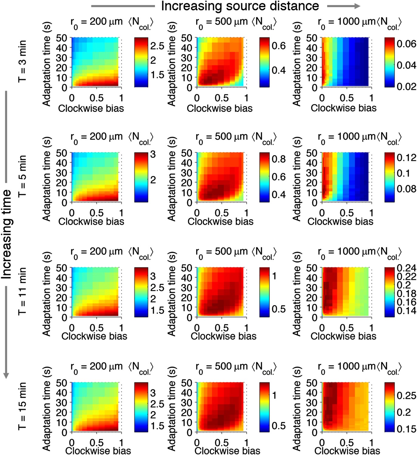
Effect of time restrictions on foraging performance.
Cells were challenged to forage sources that appeared at distances of 200, 5000, or 1000 μm away (columns from left to right). Different amounts of time were allotted to cells to accumulate ligand: 3 min, 5 min, 11 min, 15 min (rows from top to bottom). : the average nutrient collected by replicates of a given phenotype in μmol.
Figure 2—figure supplement 6
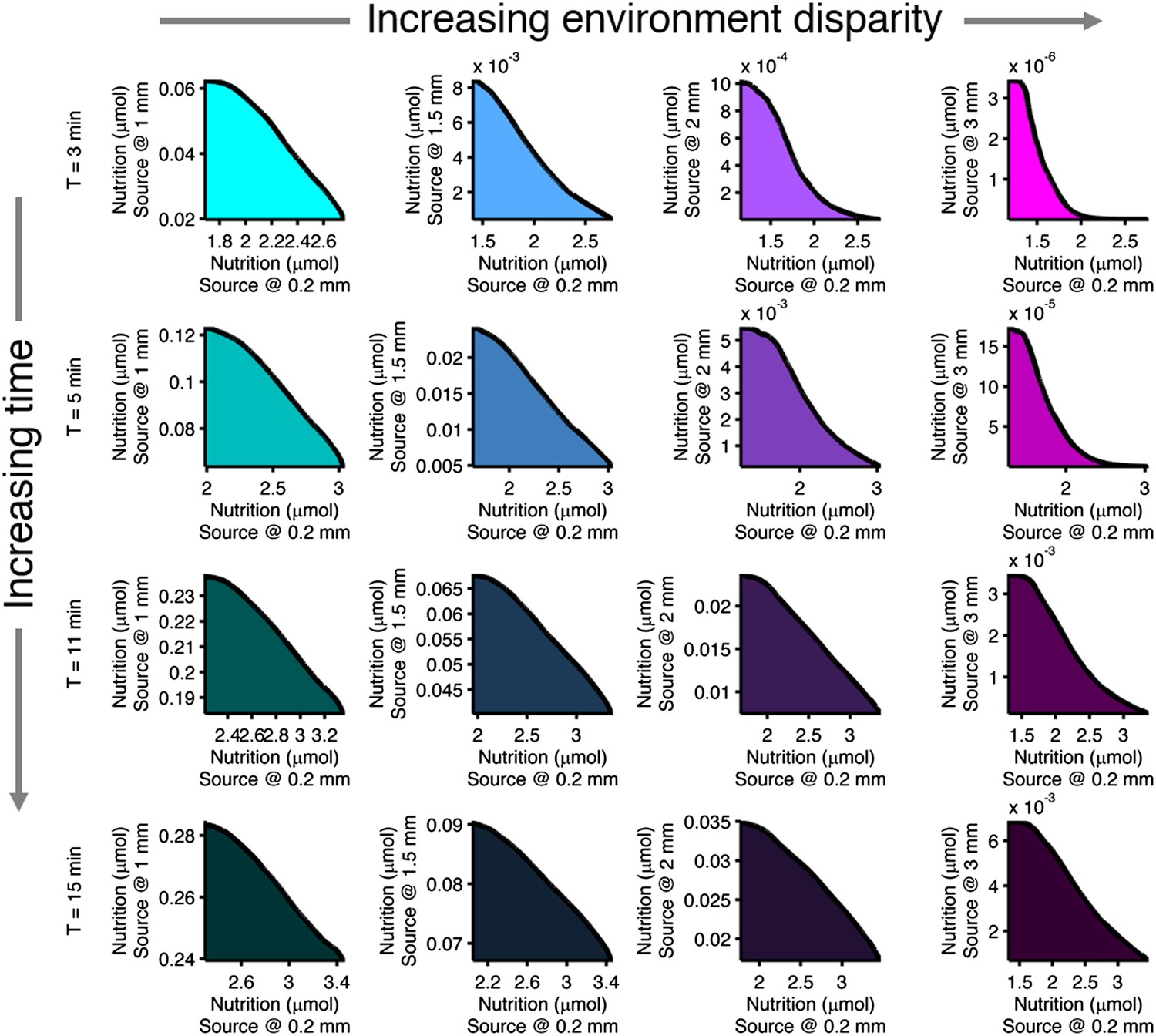
Effect of time limits on near/far foraging trade-offs.
Trade-offs in performance between foraging near and far sources are shown. From left to right (cyan to magenta), the far case is progressively more distant compared to the near case: 1 mm, 1.5 mm, 2 mm, 3 mm. From top to bottom (bright to dark colors), the time allotted is increasing: 3 min, 5 min, 11 min, 15 min. Reduced time allotment makes the front (black line) more concave for the same pair of environments.
Figure 2—figure supplement 7

Effect of source concentration on performance.
Performance calculate and plotted as described in Figure 2—figure supplement 3, but for different concentrations at the source. Left block (‘Foraging’): foraging performance for increasing source distance (columns) and increasing source concentration (rows): L1 = 1 mM, 10 mM, 100 mM. Right block (‘Colonization’) colonization performance for increasing source distance (columns) and increasing source concentration (rows): L1 = 100 µM, 1 mM, 10 mM.
Figure 2—figure supplement 8
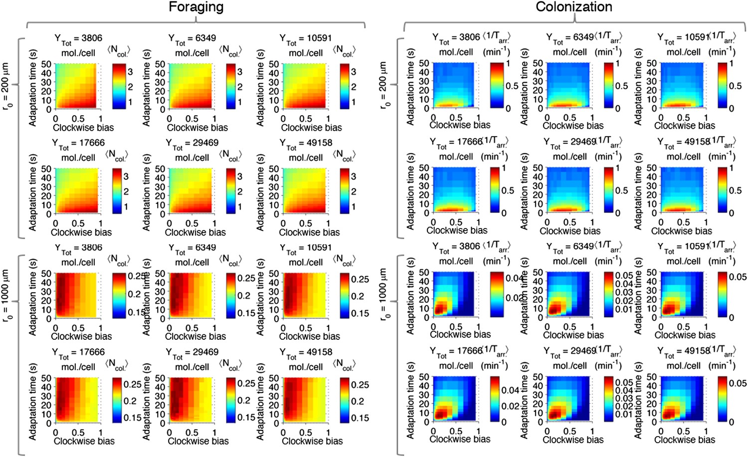
Effect of CheY-P dynamic range on performance.
Left block (‘Foraging‘): foraging performance for near (200 µm) and far (1000 µm) sources and increasing CheY-P dynamic range, which was changed through the total number of CheY molecules, Ytot, as described in the SI. Right block (‘Colonization’) same as left block but for colonization.
Figure 3
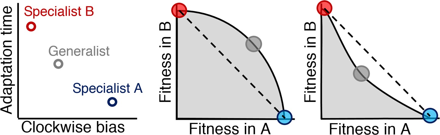
Relationship between Pareto front shape and population strategy.
Left: Two environments, A and B, select for different optimal phenotypes, specialist A and specialist B (blue and red circles). The generalist phenotype (gray circle) performs well, but not optimally, in both environments. Middle and right: Trade-off plots. Gray region: fitness set composed of the fitness of all possible phenotypes in each environment; Black line: Pareto front of most competitive phenotypes; Dashed line: fitness of mixed populations of specialists; Circles: fitness of phenotypes corresponding the circles in the left plot. Middle: In a weak trade-off (convex front), the optimal population distribution will consist purely of a generalist phenotype that lies on the Pareto front. Right: In a strong trade-off (concave front), the optimal population will be distributed between the specialists for the different environments. Here, the fitness of a mixed population of specialists (dashed line), exceeds that of the generalist in both environments.
Figure 4
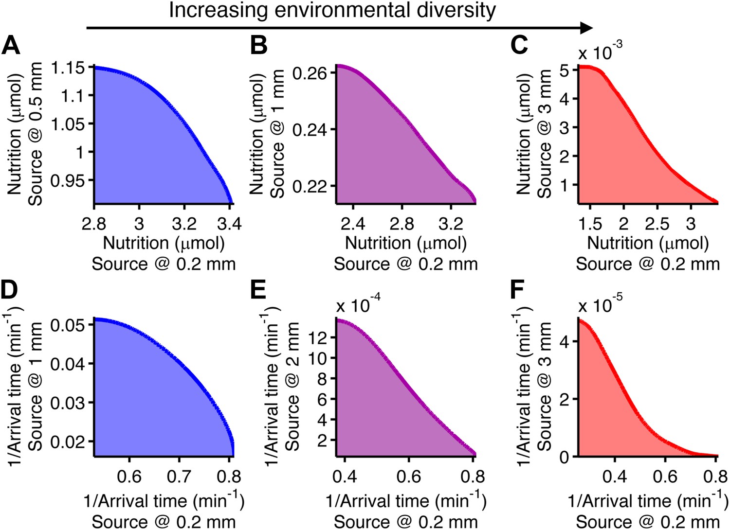
Performance trade-offs in E. coli chemotaxis.
Ecological chemotaxis tasks pose trade-off problems for E. coli that become strong when environmental variation is high. (A–C). Trade-off plot between nutrient accumulation when starting near and when starting far from a source. Plotting the performance of all possible clockwise bias and adaptation time combinations in both near and far cases (colored region) reveals the strength of the trade-off in the curvature of the front. As the disparity between starting distance becomes greater (left to right plots), the trade-off front goes from convex to concave, signifying a transition from weak to strong performance trade-offs. Source distances are indicated on axis labels. (D–F). Same as A–C but for the colonization challenge.
Figure 5 with 1 supplement
Selection can reshape trade-offs.
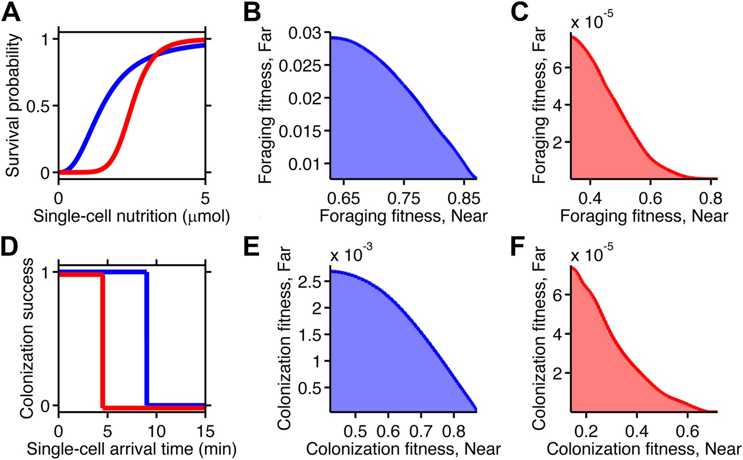
(A) Simple metabolic model of survival applied to the chemotactic foraging challenge. Each individual replicate is given a survival probability based on a Hill function of the nutrition they achieve from chemotaxis. For each phenotype, the foraging fitness is the average survival probability across replicates. The effect of more (red) and less (blue) stringent survival functions are compared. Transitional nutrition value: 1.5 µmol (blue), 2.5 µmol (red). Hill coefficient: 2.5 (blue), 7 (red). (B and C) Beginning with the neutral foraging performance trade-off in Figure 4B, application of the survival model in A gives rise to either a weak (B) or strong (C) fitness trade-off, depending on whether the thresholds and steepness are low (blue curve in A) or high (red curve in A). (D) Simple threshold model of survival applied to the chemotactic colonization challenge. Each individual replicate survives only if it arrives at the goal within the cut-off time. For each phenotype, the colonization fitness is the probability to colonize measured over all replicates. The effect of more (red) and less (blue) stringent survival functions are compared. Time threshold value: 5 min (blue), 1.5 min (red). (E and F) Beginning with the neutral colonization trade-off in Figure 4E, application of the selection model in (C) gives rise to either a weak (E) or strong (F) fitness trade-off.
Figure 5—figure supplement 1
Fitness trade-offs under alternate models of selection.
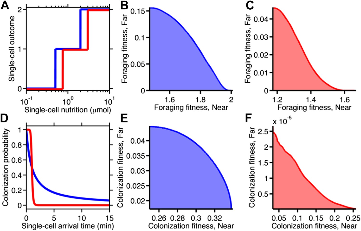
(A) Model of discrete physiological transitions applied to the chemotactic foraging challenge. Each individual replicate is given a number of progeny (0, 1, or 2) based on a two-step function of the nutrition they achieve from chemotaxis. For each phenotype, the foraging fitness is the average progeny across replicates. The effect of more (red) and less (blue) stringent nutrient requirements are compared. Survival requirement: 0.5 µmol (blue), 0.75 µmol (red), Division requirement: 2 µmol (blue), 3 µmol (red). (B and C) Beginning with the foraging performance trade-off in Figure 4B, application of the survival model in A gives rise to either a weak (B) or strong (C) fitness trade-off, depending on where the thresholds and steepness are low (blue curve in A) or high (red curve in A). D Probabilistic model of survival applied to the chemotactic colonization challenge. Each individual replicate survives has chance to survive depending on how soon it arrives. For each phenotype, the colonization fitness is the probability to colonize measured over all replicates. The effect of more (red) and less (blue) stringent survival functions are compared. Time threshold in both cases is 1 min with dependency 1 (blue) or 10 (red). (E and F) Beginning with the arrival performance trade-off in Figure 4E, application of the selection model in C gives rise to either a weak (E) or strong (F) fitness trade-off.
Figure 6
Genetic control of phenotypic diversity.
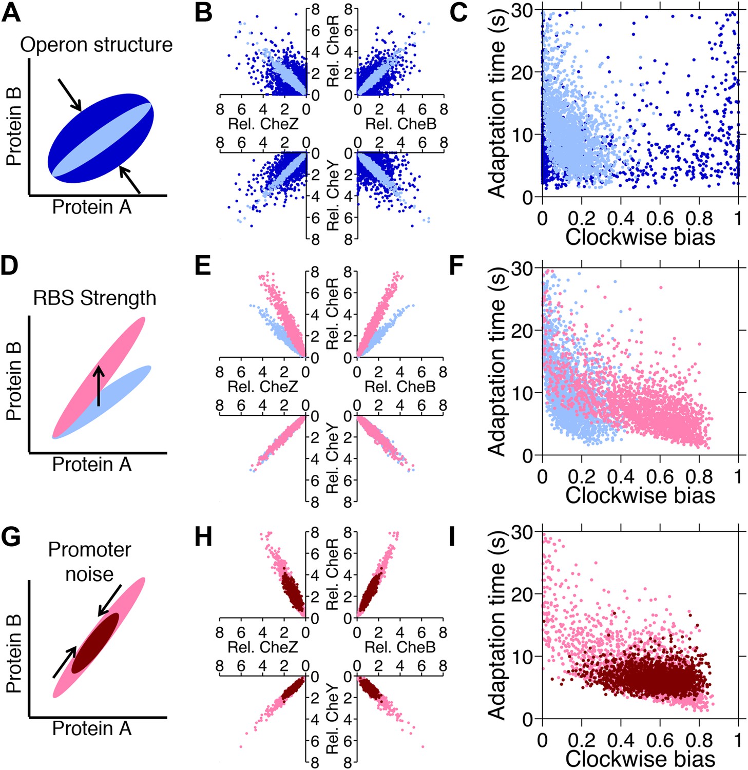
(A) Clustering genes on multicistronic operons constrains the ratios in protein abundance. (B) Protein expression of core chemotaxis proteins CheRBYZ are shown relative to the mean level in wildtype cells. Two thousand cells are plotted. Light blue: mean levels of the proteins CheRBYZAW and receptors are equal to the mean levels in wildtype cells, which we take to be 140, 240, 8200, 3200, 6700, 6700, 15,000 mol./cell, respectively (Li and Hazelbauer, 2004); the extrinsic noise scaling parameter, ω, is 0.26 and the intrinsic noise scaling parameter, η, is 0.125, which are both equal to wildtype levels (Figure 2—figure supplement 1). Dark blue: same but with ω = 0.8, which is greater than wildtype level. Note the substantial variability around the mean even in the case of wildtype noise levels (light blue). (C) Clockwise bias and adaptation time of individuals in (A). (D) Changes in the strength of individual RBSs will independently change the mean levels of individual proteins. (E and F) Light blue: gene expression of cells with same population parameters as in A, light blue. Pink: mean levels of CheR changed to twice wildtype mean. (G) Promoter sequences can be inherently more or less noisy, resulting in amplification or attenuation of the variability of total protein amounts without affecting protein ratios. (H and I) Pink: gene expression of cells with same population parameters as in (E), pink. Red: ω reduced from 0.26 to 0.1.
Figure 7
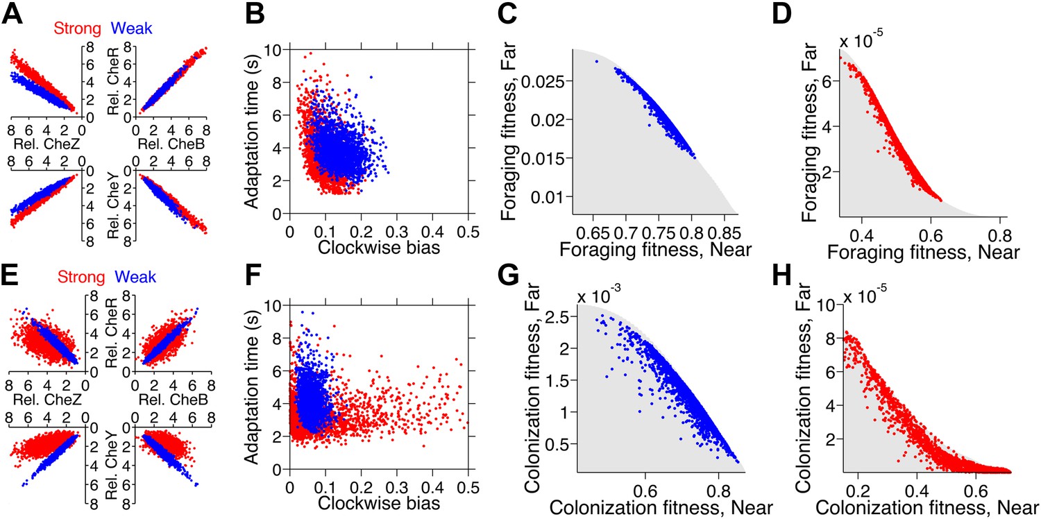
Optimization of gene expression noise reshapes population distributions to the Pareto front.
Protein expression of populations were optimized for either weak or strong foraging fitness trade-offs (same trade-offs as in Figure 5B,C). For each population, 2000 individuals are plotted, protein expression shown relative to the mean level in wildtype cells. (A) Gene expression parameters of the population optimized for the weak foraging trade-off: mean expression levels of CheRBYZAW and receptors relative to mean wildtype expression level were 2.54, 2.53, 2.50, 4.20, 4.50, 3.49, and 3.49 fold, respectively, with an intrinsic noise scaling parameter, η, of 0.051 and an extrinsic noise scaling parameter, ω, of noise 0.128. For the strong foraging trade-off: mean CheRBYZAW and receptors relative to wildtype were 3.27, 3.27, 2.86, 3.83 4.17, 2.82, and 5.00 fold, respectively, with η = 0.051 and ω = 0.200. (B) Clockwise bias and adaptation time of individuals in A with the corresponding dot color. (C) Fitness of the population that was optimized for the weak foraging trade-off (corresponding to blue dots in A and B). (D) Same as C but for the population optimized for the strong foraging trade-off. (E–H) Same as (A–D) for the colonization fitness trade-offs shown in Figure 5E,F. Population parameters optimized for weak colonization trade-off: mean CheRBYZAW and receptors levels relative to wildtype were 2.42, 2.52, 2.32, 2.50, 4.16, 3.25, and 5.00 fold, respectively, with η = 0.055 and ω = 0.126. Population parameters optimized for strong colonization trade-off: mean CheRBYZAW and receptors levels were 2.90, 2.92, 1.71, 3.845, 2.25, 3.80, and 3.76 fold, respectively, with η = 0.221 and ω = 0.090.
Additional files
-
Supplementary file 1
Parameter values.
- https://doi.org/10.7554/eLife.03526.019
Download links
A two-part list of links to download the article, or parts of the article, in various formats.
Downloads (link to download the article as PDF)
Open citations (links to open the citations from this article in various online reference manager services)
Cite this article (links to download the citations from this article in formats compatible with various reference manager tools)
Adaptability of non-genetic diversity in bacterial chemotaxis
eLife 3:e03526.
https://doi.org/10.7554/eLife.03526


