Mapping nonlinear receptive field structure in primate retina at single cone resolution
- Howard Hughes Medical Institute, United States
- Center for Neural Science, United States
- Duke University School of Medicine, United States
- Salk Institute for Biological Studies, United States
- University of Oldenburg, Germany
- University of Strathclyde, United Kingdom
- University of California, Santa Cruz, United States
- Columbia University, United States
- Courant Institute of Mathematical Sciences, United States
- Stanford School of Medicine, United States
Figures
Figure 1

Failure of linear integration in OFF midget retinal ganglion cells (RGCs).
(A) Above, spatial spike-triggered average derived from white-noise analysis with high-resolution pixel stimulation. Black lines indicate regions of pixels independently stimulating individual cones (identified online). White line, scale bar (8.4 microns). Below, rasters of responses to repeated brief presentations of uniform luminance within each cone region. Each row is a trial, each point is a spike. Black line, average firing rate across trials. Gray line, stimulus presentation (250 ms). Stimulation in cone regions was either paired increments and decrements of light, or decrements alone, as shown in insets. (B) Another RGC showing failure of cancellation. (C) A RGC exhibiting cancellation.
Figure 2
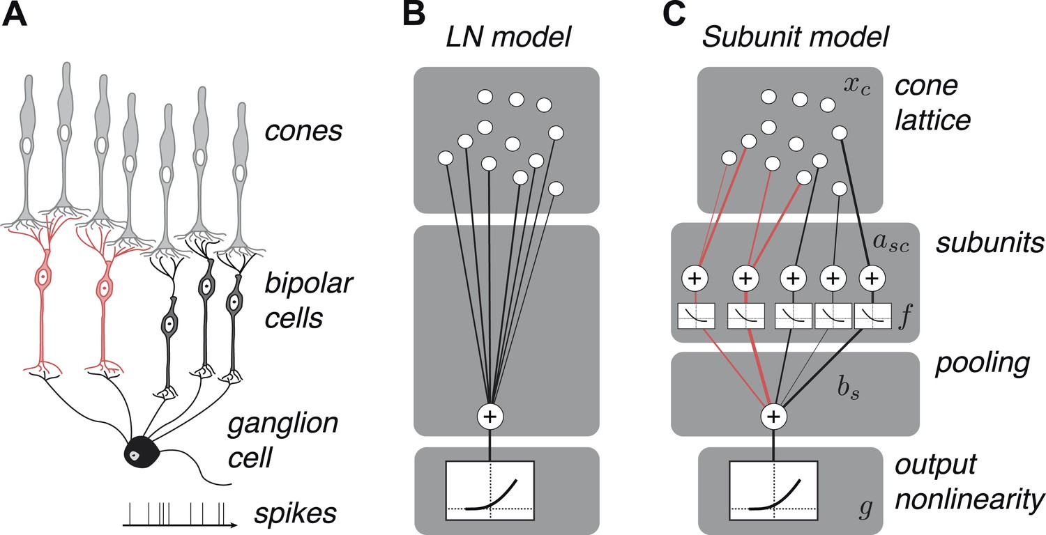
OFF midget RGC anatomy and modeling framework.
(A) Bipolar cells receive convergent input from cones, and ganglion cells receive convergent input from bipolar cells. (B) A linear–nonlinear (LN) model describes the RGC response with one stage of linear integration of cone inputs, followed by a nonlinearity. White disks indicate cones, black line indicates integration weights. (C) The subunit model describes the RGC response with two stages of linear integration and nonlinearity; subunits perform initial integration following by a nonlinearity (common to all subunits). Red, subunits receiving input from two cones; black, subunits receiving input from one cone. Cones are indexed by c, subunits by s. xc is the input to each cone. asc is the weight from cone c to subunit s. bs is the weight on each subunit. f and g are the subunit and spiking nonlinearities, respectively. See ‘Materials and methods’ for details on parameterization and fitting.
Figure 3 with 1 supplement
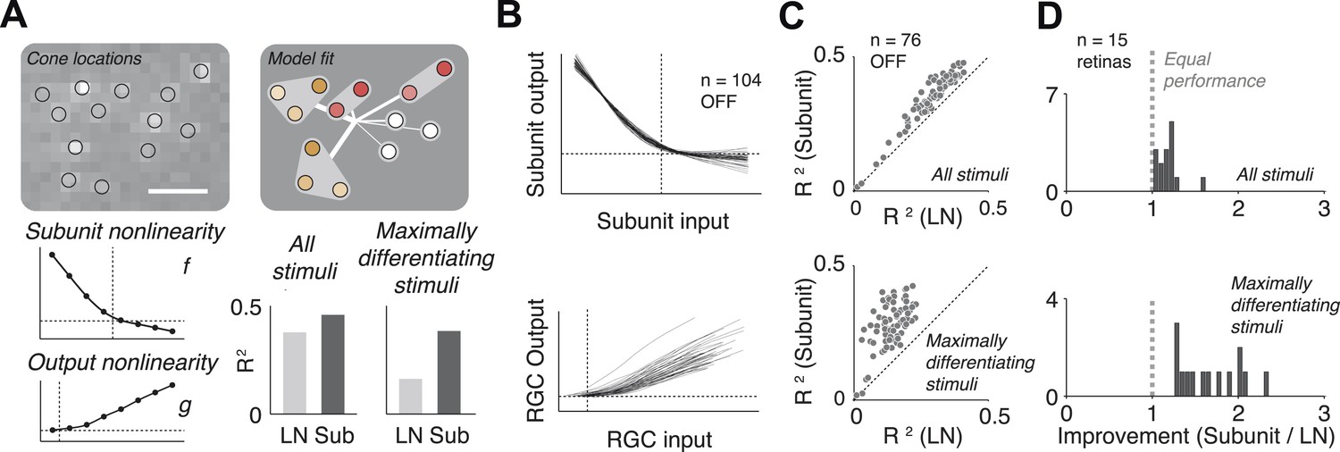
Model fits.
(A) Recovered model fit for an example OFF midget RGC. Top left, spatial spike-triggered average. Identified cone locations indicated by black circles. White line, scale bar (8.4 microns). Top right, diagram of model fit. Light gray regions indicate subunits, including those containing single cones. Within a subunit, color saturation indicates the weight on each cone. Red indicates that the subunit has two cones, orange, three. Line intensities indicate weights used in summing over subunits. Bottom left, recovered subunit and output nonlinearity. Bottom right, explanatory power (R2, see ‘Materials and methods’) of LN and subunit (‘Sub’) models. R2 was computed either for all presented stimuli, or for maximally differentiated stimuli, defined as those stimuli for which the predictions of the two models differed the most (see ‘Materials and methods’); in both cases models were evaluated on data not used for model fitting. (B) Summary of subunit and output nonlinearities for a population of 104 OFF midgets from one retina. Each line corresponds to a single RGC. Nonlinearities only shown for RGCs with R2 exceeding 0.2. (C) Summary of model performance for 76 OFF midget RGCs from an example retina. Above, R2 for subunit and LN models on all stimuli; below, R2 for subunit and LN models on maximally differentiating stimuli (see panel A, and ‘Materials and methods’). Each corresponds to a single RGC. (D) Histogram of model improvement (subunit/LN) across multiple retinas, quantified for each retina as the slope of the best-fitting regression line to the points shown in panel C (forced through the origin). The data point for OFF midgets from one outlying retina (improvement = 5) is not shown.
Figure 3—figure supplement 1
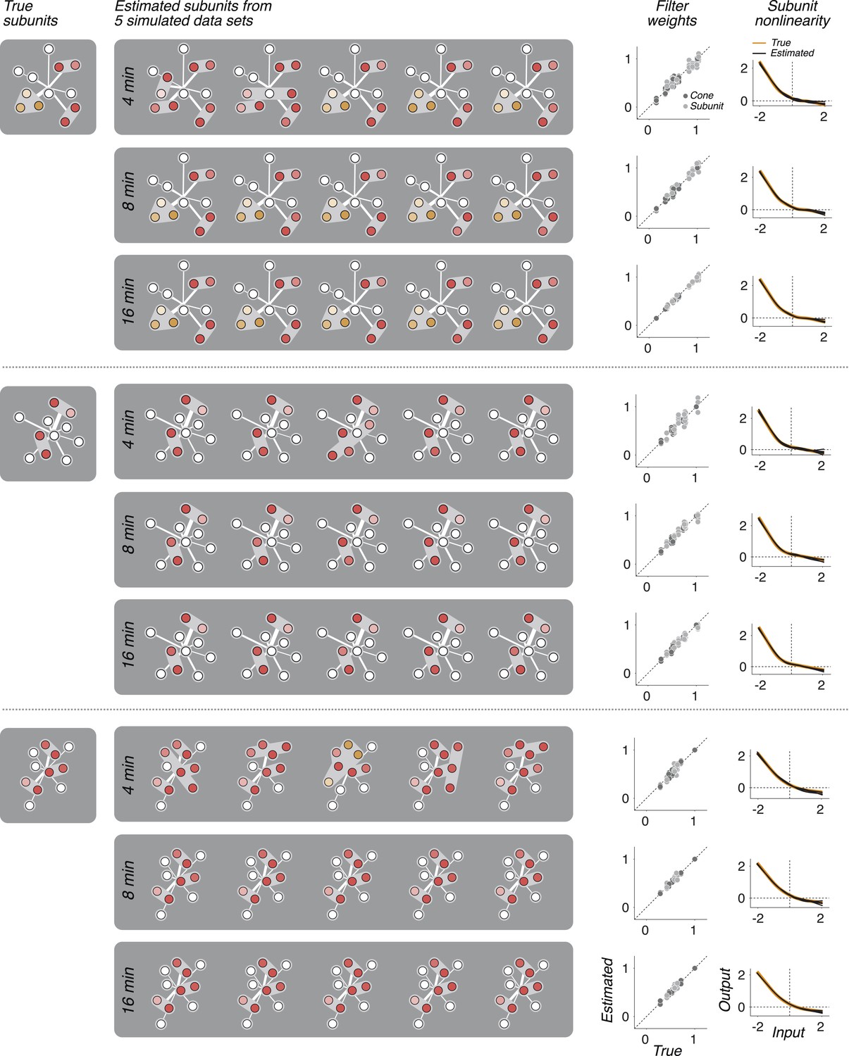
In three separate simulations, spiking responses were simulated using a known set of parameters (derived from the model fit to a real OFF midget RGC), and simulation duration was either 4, 8, or 16 min (typical experiments were 30 min).
The model was then fit to these simulated responses. The process was repeated five times for each simulation and duration, yielding five sets of recovered parameters: subunit assignments, weights (on cones and subunits), and nonlinearities. In cases where the fitted subunit assignments did not match the true assignment, the true assignment was used to infer weights and nonlinearities beacuse otherwise comparing to the true values is not well defined. Fitted subunits depicted as in Figures 3, 6, 7. The recovered parameters in all cases were found to be similar to the parameters used in simulating the data. In particular, with 8 or 16 min of data, accurate subunit assignments are nearly always recovered.
Figure 4
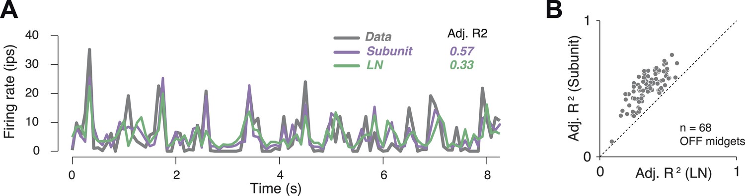
Subunit model predicted responses to repeated white noise.
(A) Average firing rate of a single OFF midget RGC to an 8 s white noise stimulus repeated 100 times. Purple, prediction of subunit model; green, prediction of LN model. Both models were fit to independent data using non-repeated white noise stimuli. Bin width, 83 ms. (B) Adjusted R2 (see ‘Materials and methods’) for the two models; each point shows performance for one OFF midget RGC.
Figure 5
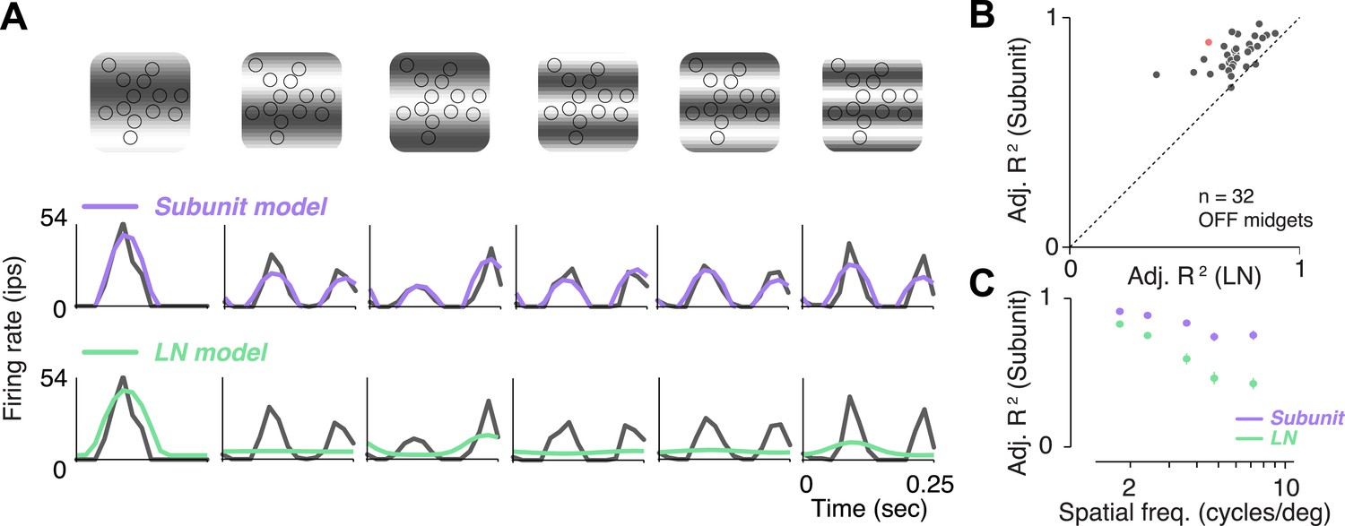
Responses to gratings.
(A) Sinusoidal gratings temporally modulated in contrast were presented to OFF midget RGCs. Top: grating stimuli superimposed on the cone locations of a single RGC, for a set of example combinations of spatial frequency and phase (with spatial frequency increasing from left to right). Bottom: cycle-averaged firing rate of the RGC (black); predictions of the LN model (green); predictions of the subunit model (purple). Both models were fit to independent data from white-noise stimulation. (B) Performance (adjusted R2, see ‘Materials and methods’) for subunit and LN models, across 32 OFF midget RGCs from a single retina. Data point in red corresponds to example shown in panel A. (C) Adjusted R2, computed separately for the two models for different spatial frequencies, averaged across RGCs. Error bars indicate s.e.m. across RGCs.
Figure 6
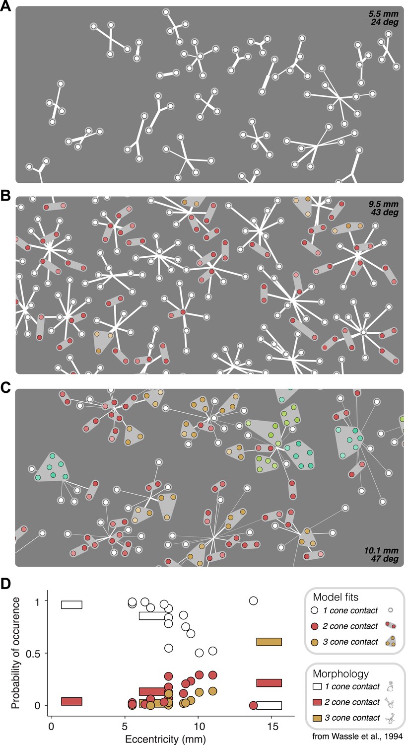
Recovered subunit structure varies with eccentricity.
(A–C) Model fits recovered for local populations of OFF midget RGCs from retinas at three different retinal eccentricities. Model fits for each RGC depicted as in Figure 3. Colors indicate the number of cones in each subunit; white = 1, red = 2, orange = 3, lime = 4, turquoise = 6. (D) Probability of occurrence of subunits with different numbers of cone contacts as a function of eccentricity, for morphological and functional data. Horizontal bars show estimates derived from morphological data from Wässle et al., 1994. Circles show estimates from the functional measurements and model fitting for individual retinas.
Figure 7
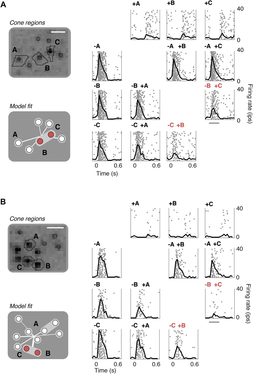
Closed-loop validation of subunit organization.
(A) Upper left, spatial spike-triggered average and cone stimulation regions, as in Figure 1. Lower left, diagram of fitted subunit model, as in Figure 3A. The three cones (A, B, C) were stimulated with increments (+) or decrements (−) of light. Panels on the right show the responses (as in Figure 1) of a single OFF midget RGC to different combinations of light increments and decrements. Top row, and left column, show responses to stimulation of single cones. Remaining panels show responses to paired stimulation. Red indicates the pair of cones found by the model to belong to a single subunit, and thus selected for paired stimulation. Gray line, stimulus presentation (250 ms). (B) Another example, plotted as in panel A.
Author response image 1
Download links
A two-part list of links to download the article, or parts of the article, in various formats.
Downloads (link to download the article as PDF)
Open citations (links to open the citations from this article in various online reference manager services)
Cite this article (links to download the citations from this article in formats compatible with various reference manager tools)
Mapping nonlinear receptive field structure in primate retina at single cone resolution
eLife 4:e05241.
https://doi.org/10.7554/eLife.05241


