Dynamics of preventive vs post-diagnostic cancer control using low-impact measures
- University of Montpellier, France
- McMaster University, Canada
- Santa Fe Institute, United States
- Wissenschaftskolleg zu Berlin, Germany
Figures
Figure 1

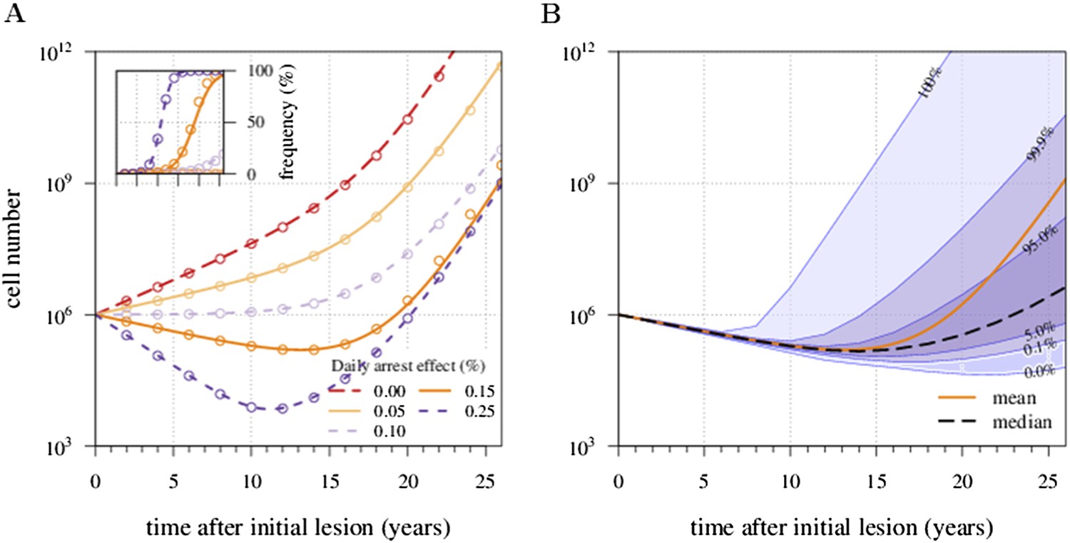
Treatments curb or eliminate tumours.
Examples of single patient tumour growth for (A) no treatment. (B) σ = 0.6%. (C) σ = 1.0%. (D) σ = 2.0%. The shaded area shows the change in total tumour size and the hatched area, the resistant part of a tumour. The treatment intensity σ in this and all other figures are represented as cell arrest per day (σ/4). Parameter values as in Table 1.
Figure 2 with 2 supplements

Treatment level affects both detection time and frequency of resistance.
The median (lines) and 90% confidence intervals (shaded areas) of detection times, measured as years beyond the initiation of the preventive measure. Effects of: (A) the selective advantage of each additional driver and (B) the cost of resistance. (C) Samples of the distribution of detection times (in relative frequencies, adjusted for 3-month bins) for corresponding points, indicated in A and B. Dashed black line is the mean and the dashed-and-dotted line is the median. The colour-code indicates the average level of resistance in detected tumours over 3 month intervals (see inset in B). All cells j = 0 at t = 0. Other parameters as in Table 1. Detection time is log-transformed in A and B.
Figure 2—figure supplement 1
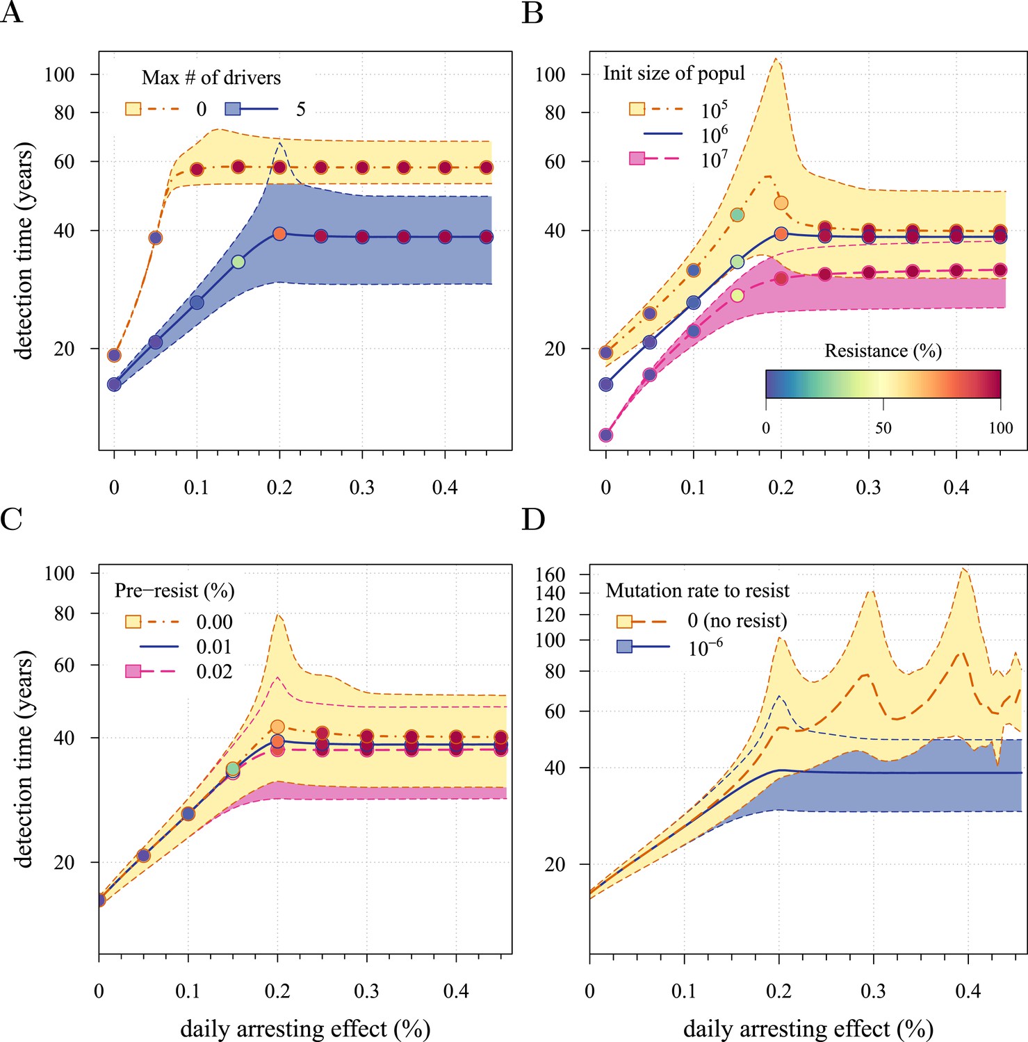
Sensitivity analysis for several key parameters.
(A) Maximal number of additionally accumulated drivers. (B) Initial cell number. (C) Level of initial partial resistance of a tumour. (D) Presence or absence of resistant cell-lines. Point colour-codes indicate the average level of resistance in detected tumours over 3 month intervals (see inset in B). For simplicity, only the median is indicated in B and C for the baseline case (blue line). Lines and shading otherwise as in Figure 2. Unless otherwise stated, parameter values as in Table 1.
Figure 2—figure supplement 2
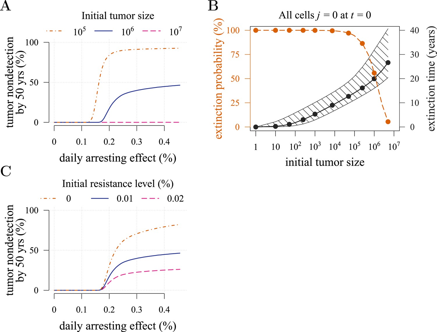
Effects of initial neoplasm size (A, B) and resistance level (C) on preventive measure success.
Success is defined as tumour non-detection by 50 years. Daily effect of treatment on cellular arrest is assumed to be 0.25%. Unless otherwise stated, parameter values as in Table 1.
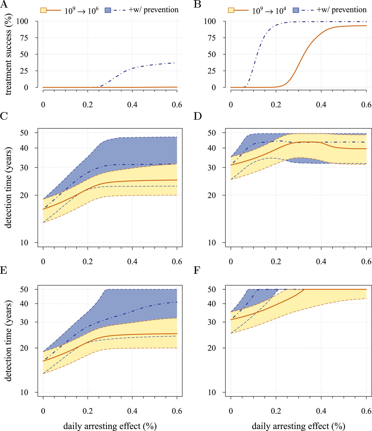
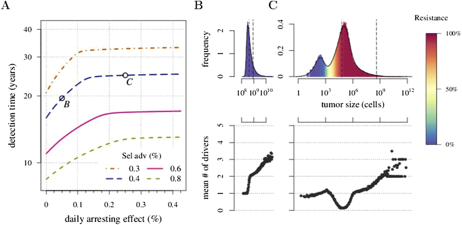
Figure 3 with 5 supplements
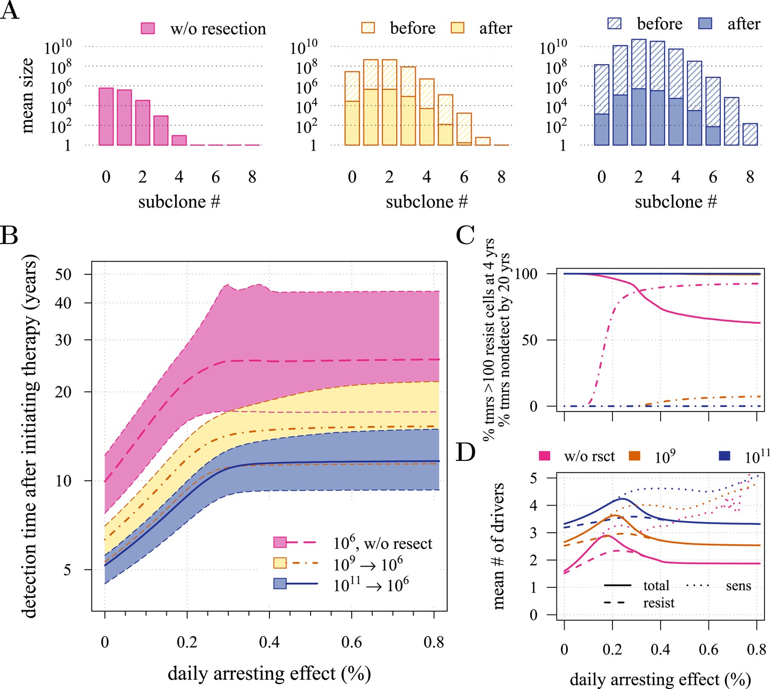
Effects of preventive and post-diagnostic interventions against tumours consisting of 1 million cells.
(A) The distribution of mean sizes of subclones (hatched bars = before removal and solid bars = post removal). (B) The time distribution of cases in which either intervention type fails to control the tumour below the detection threshold after 50 years (thick line = median, filled area with dashed boundaries = 90% CIs) for different constant treatment intensities. (C) The percentage of cases where the tumour consists of less than 100 resistant cells at 4 years after treatment commences (solid lines), and the percentage of cases where tumour size is below the detection threshold 20 years after the measure begins (dashed-and-dotted lines). (D) The mean number of accumulated drivers within a tumour at the time of detection. Parameter values as in Table 1.
Figure 3—figure supplement 1
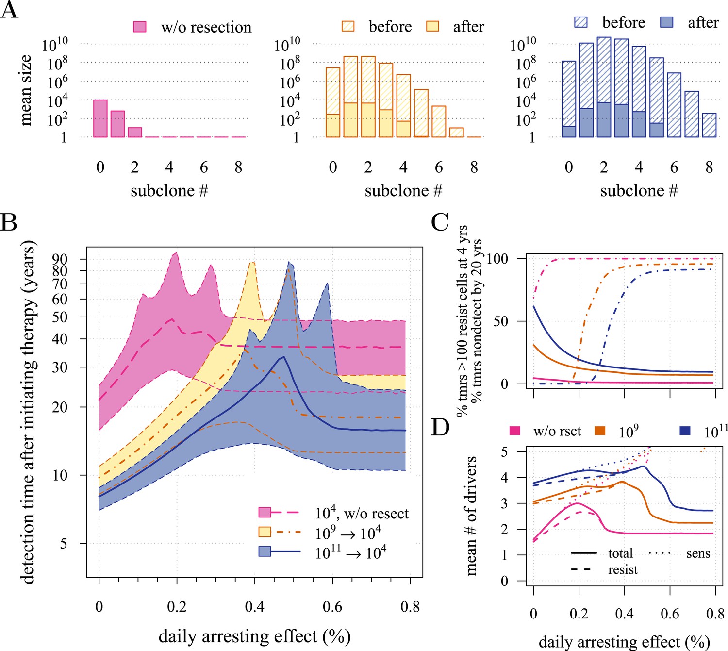
Effects of preventive and post-diagnostic interventions against tumours consisting of 10,000 cells.
Same as Figure 3, except interventions against 104 cancer cells. (A) The distribution of mean sizes of subclones for different constant treatment intensities (hatched bars = before removal and solid bars = post removal). (B) The time distribution of cases in which either intervention type fails to control the tumour below the detection threshold after 50 years (thick lines = medians, shaded areas with dashed boundaries = 90% CIs). (C) The percentage of cases when a tumour consists of less than 100 resistant cells at 4 years post-resection (solid lines) and the percentage of cases when tumour sizes are below the detection threshold 20 years after the measure commences (dashed-and-dotted lines). (D) The mean number of accumulated drivers within a tumour at the time of detection. Parameter values as in Table 1.
Figure 3—figure supplement 2
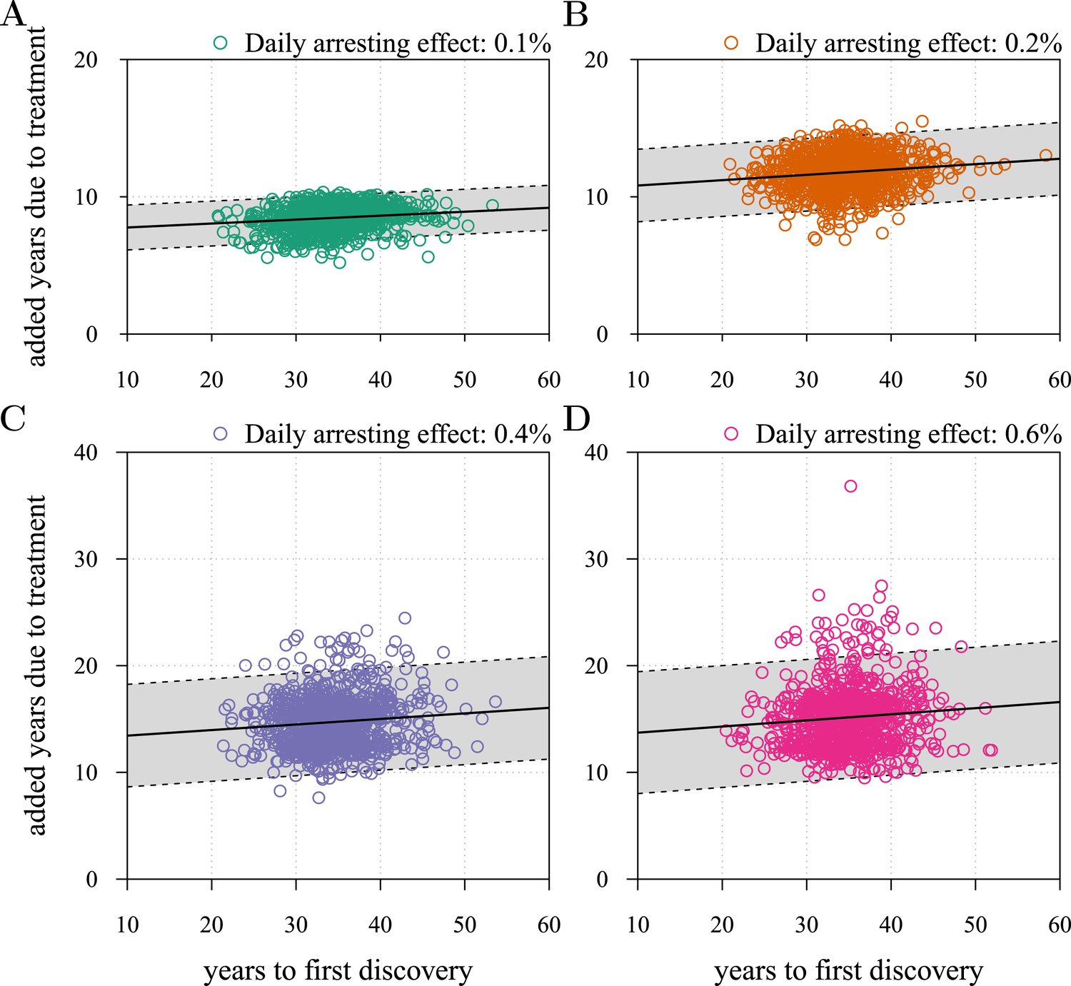
Time to first discovery as a predictor of post-diagnostic treatment success.
Time to tumour relapse following resection as function of the time it takes for the initial cancer cell to attain 109 cells (i.e., the point at which the tumour is discovered, resected, and treatment begins). Each dot represents a numerical simulation from the yellow distribution in Figure 3B (only 1,000 simulation results out of 106are shown). Four different treatment levels are considered. Black solid line is a simple linear regression, and grey area with dashed boundaries indicates extrapolation of high and low bounds accounting for 95% of observations (prediction interval). The fitted linear regression model gives an intercept of 7.5 years, a slope of 1.6° and R2 of 0.024 in (A), 10.4 years, 2.2° and R2 of 0.017 in (B), 12.9 years, 3.0° and R2 of 0.009 in (C), and 13.1 years, 3.3° and R2 of 0.008 in (D). Parameters as in Table 1.
Figure 3—figure supplement 3
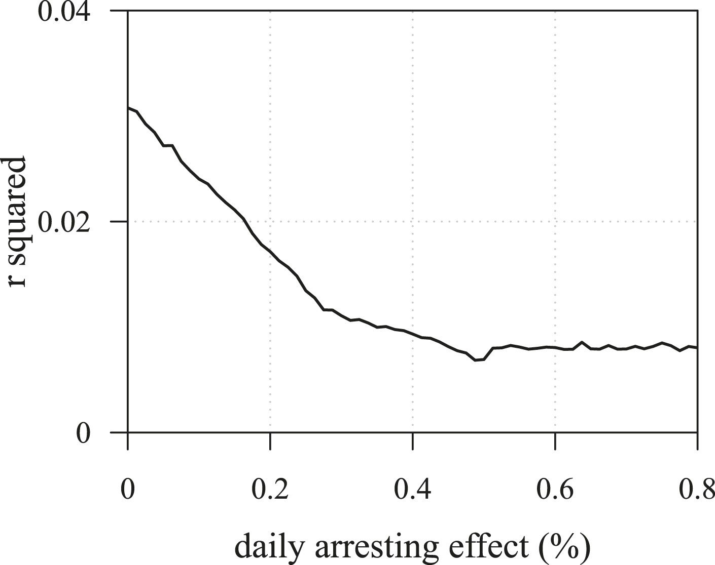
The R2 of regressions from numerical experiments for different treatment levels of time to tumour relapse following resection as function of the mean number of drivers in a resected tumour.
Time to tumour discovery is generally more predictive of post-diagnostic therapeutic outcome for lower treatment levels. See Figure 3—figure supplement 2 for details.
Figure 3—figure supplement 4
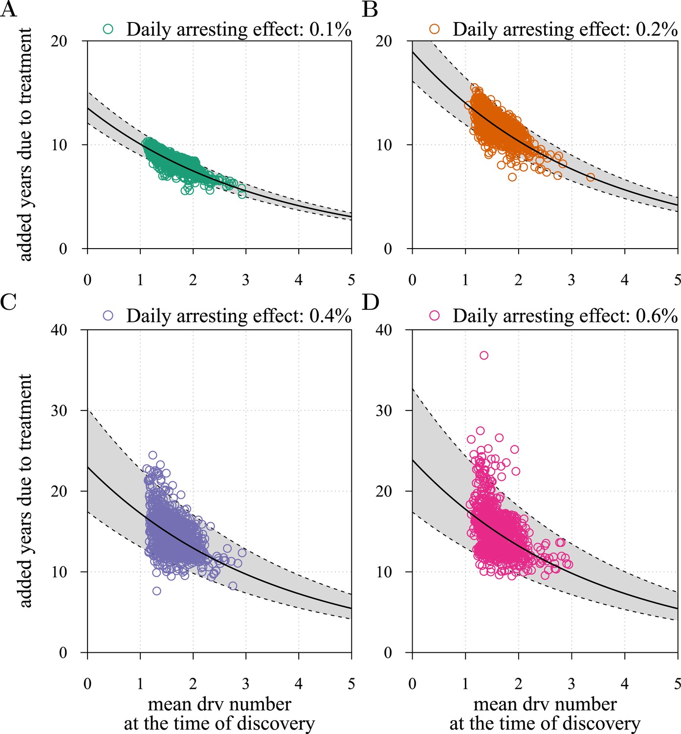
Mean number of additionally accumulated drivers in resected tumour as a predictor of post-diagnostic treatment success.
The fitted negative exponential regression model y = ae-bx gives a = 13.5 years, b = 0.3 and R2 = 0.696 in (A), 18.95 years, 0.3 and R2 = 0.537 in (B), 23.0 years, 0.29 and R2 = 0.262 in (C), and 23.9 years, 0.3 and R2 = 0.224 in (D). See Figure 3—figure supplement 2 for details.
Figure 3—figure supplement 5
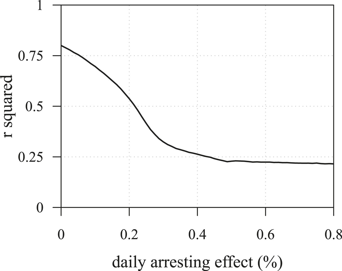
The R2 of regressions from numerical experiments for different treatment levels of time to tumour relapse following resection as function of the mean number of drivers in a resected tumour.
Time to tumour discovery is more predictive of post-diagnostic therapeutic outcome for lower treatment levels. See Figure 3—figure supplement 4 for details.
Figure 4
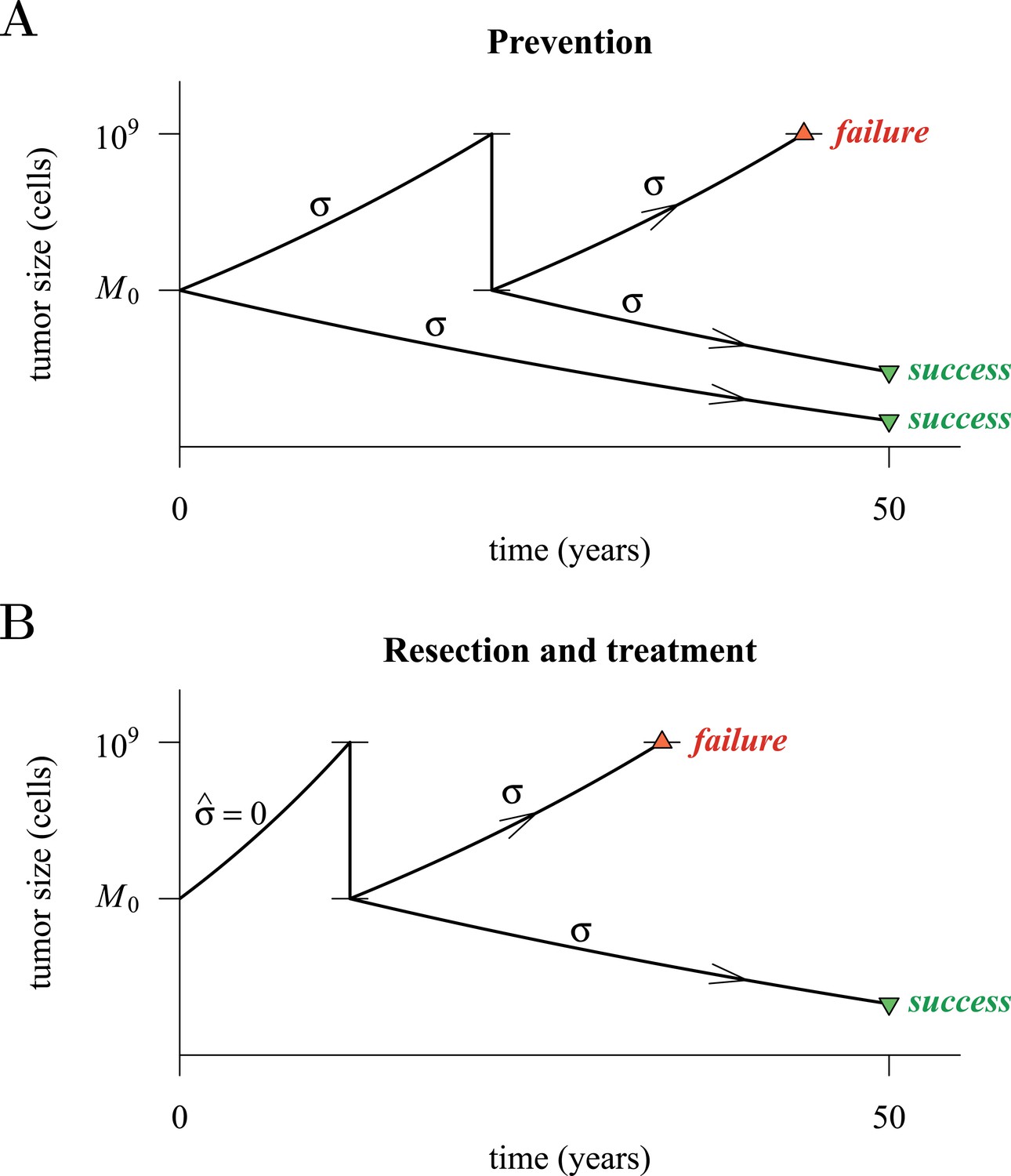
Hypothetical process of preventive (with a ‘second chance’) and post-diagnostic measures.
A tumour is initiated by one cell and grows to size M0 (either 104 or 106 cells in our numerical studies). Prevention (A) arrests tumour growth at intensity σ (daily level = σ/4). Should the tumour grow to 109 cells, it is diagnosed and resected to M = M0 cells and then treated again at intensity σ. Post-diagnostic intervention (B) does not discover the growing tumour until 109 cells (i.e., ), whereupon it is resected to M = M0 cells and then treated at intensity σ > 0. Either intervention finally ‘fails’ should the tumour attain 109 cells a second time, no later than 50 years after the initial lesion of size M0. Should the tumour be eradicated or not exceed 109 cells by 50 years after the initial lesion, then the intervention is deemed a ‘success’.
Figure 5 with 3 supplements
Comparison of preventive (blue lines and shading) and post-diagnostic (red lines, yellow shading) interventions.
Tumours are either treated at M0 = 106 cells (left panels) or M0 = 104 cells (right panels). (A, B) Probability of treatment success, defined as the proportion of cases where the tumour remains undetected (either extinct or below 109 cells) by 50 years after the initial lesion of M0 cells. (C, D) Distribution of times to relapse for treatment failures. (E, F) Distribution of detection times for all cases including relapsed tumours and tumours remaining undetected prior to and after 50 years (detection times are assigned to 50 years in the latter case). Parameters as in Table 1. See Figure 3 for details.
Figure 5—figure supplement 1
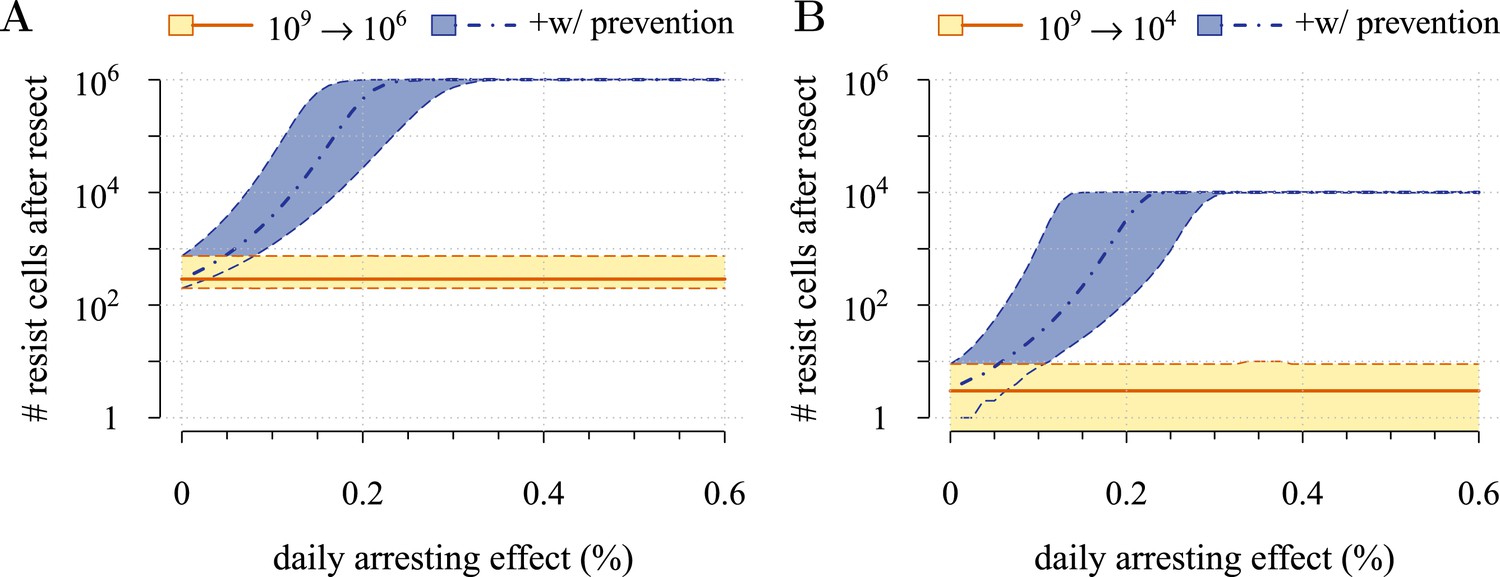
Resistant cell populations after initial failure.
Tumours are either treated at M0 = 106cells (A) or M0 = 104cells (B). Red lines and yellow shading = population following resection. Parameter values as in Table 1.
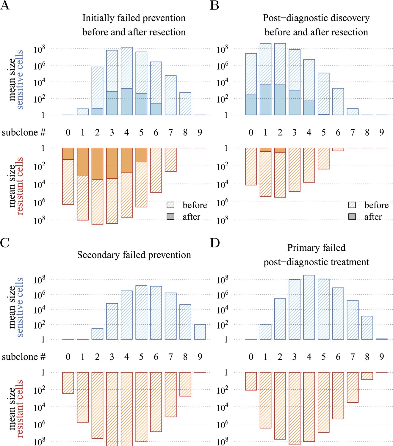
Figure 5—figure supplement 2
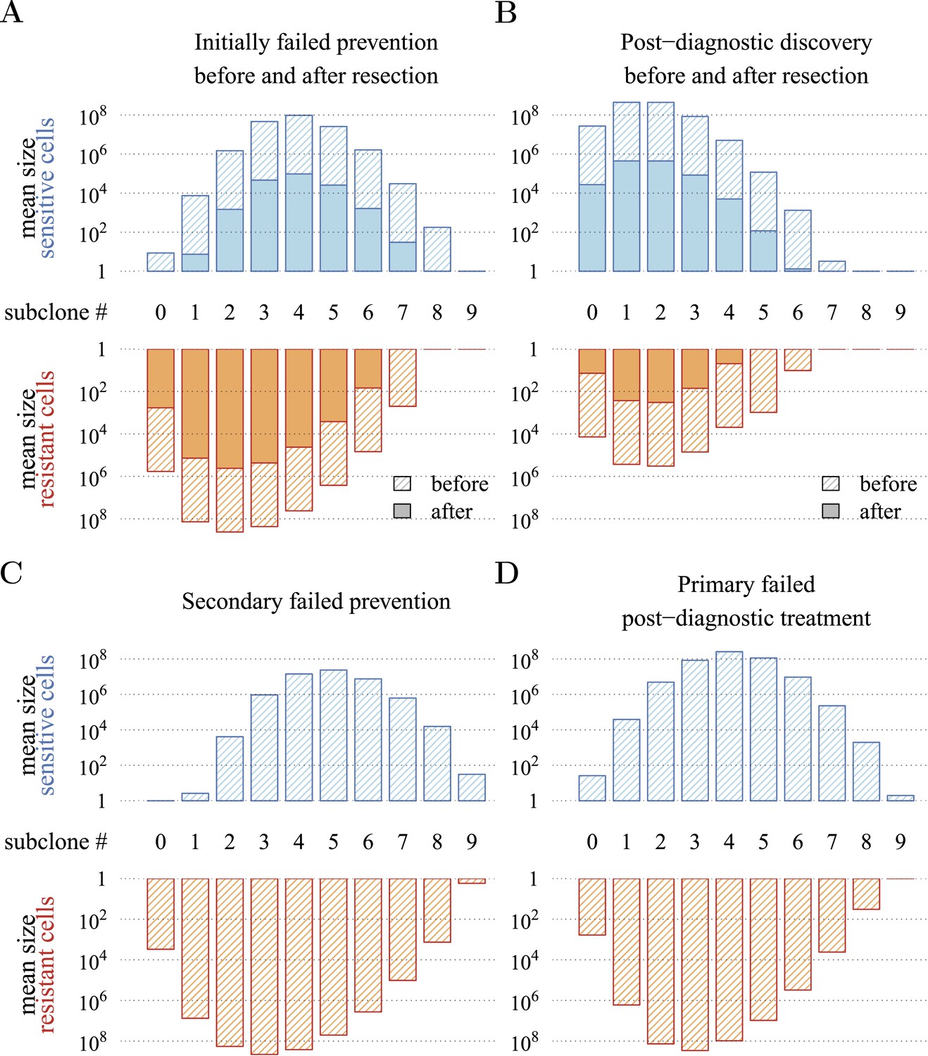
Distribution of mean sizes of subclones.
(A) Cases where a tumour is detected and resected following prevention. (B) Cases where a tumour is detected and resected with no prevention. (C) Cases of relapse following resection and secondary treatment to initially failed prevention. (D) Cases of relapse following resection and primary treatment in cases where there was no prevention. Hatched bars indicate cell numbers in the tumour and solid bar numbers after resection and 106 residual or metastatic cells. Daily arresting level assumed to be 0.25%. Parameter values as in Table 1.
Figure 5—figure supplement 3
Distribution of mean sizes of subclones.
Same as Figure 5—figure supplement 2, except M0 is 104 cancer cells.
Figure 6
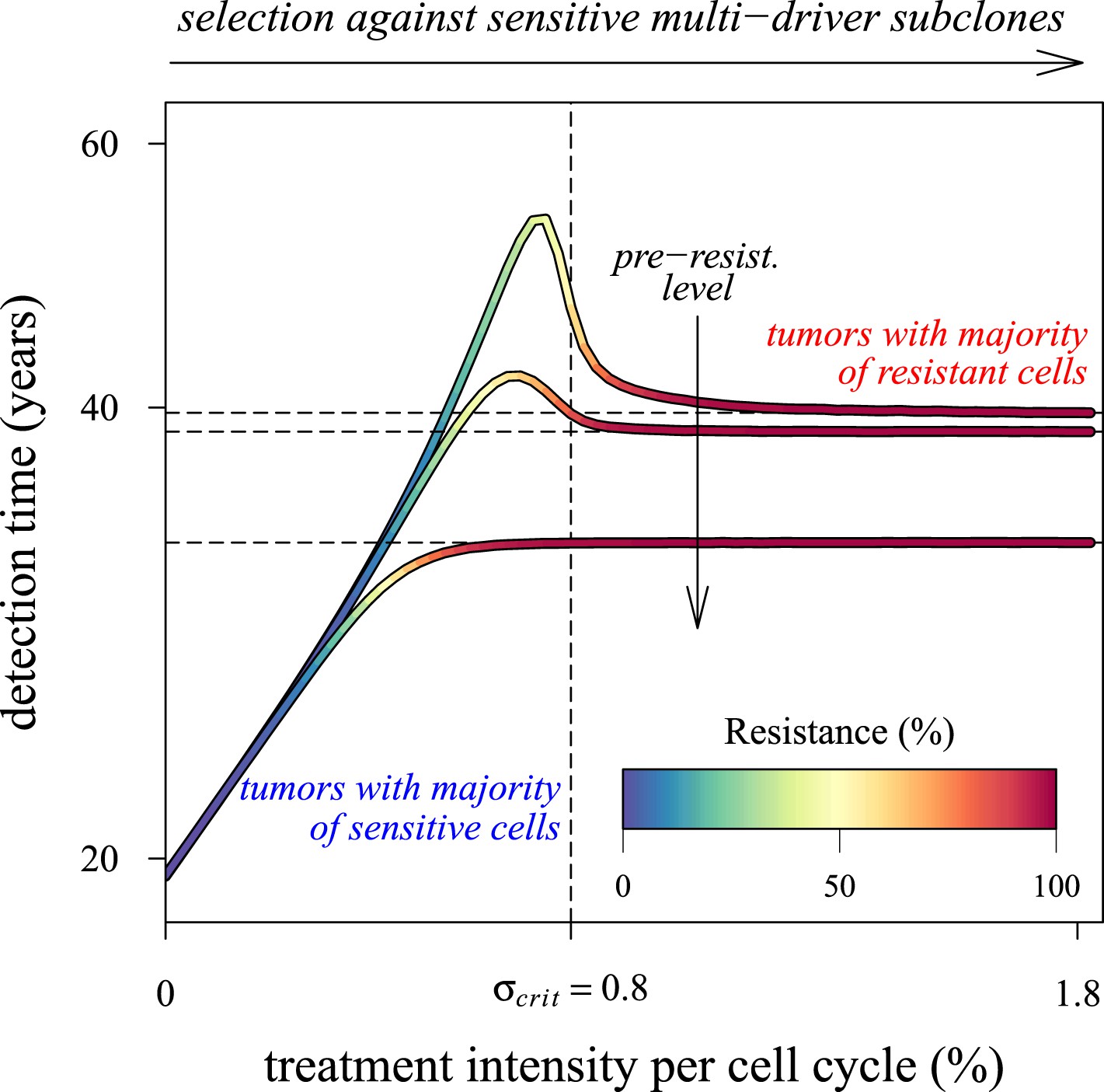
Dependence of the median time for tumour detection on treatment intensity and pre-resistance levels.
Increasing treatment intensity selects against subclones with increasing numbers of drivers, whereas, regardless of treatment intensity, all resistant subclones with s(i+1) > c increase in number. The solid lines illustrate how selection and the initial number of resistant cells in a treated tumour predict median detection times and associated resistance levels. Median detection times approach a horizontal asymptote at 100% resistance as treatment intensity increases, whereas if the resistant mutation were to be knocked out, then the vertical asymptote at σcrit = qs (where q is the number of drivers in the fastest growing subclone) would be approached instead for sufficiently small tumours. Asymptotes are shown as dashed lines. We illustrate three cases, each with an initial population of 100,000 identical cells (i = 0) and with one of three different initial numbers of resistant cells: 10, 100 or 1,000 (top to bottom lines). Other parameters as in Table 1.
Appendix 1—figure 1
Mean field dynamics concord with numerical simulations.
(A) Effect of treatment level and observation time on mean tumour size. (Inset) Mean frequency of resistant cells within tumours corresponding to three of the cases in A. Lines are analytically computed mean-field trajectories, while dots are numerical simulations (see Appendix 1 for details). (B) Dynamics of mean and median tumour size, and percentiles around the median (shaded areas), assuming a fixed constant arresting effect of 0.15% / day. Treatments start at t = 0, and the maximal number of additionally accumulated drivers is 3. See Table 1 for other parameter values.
Appendix 1—figure 2
Trade-off between growth and resistance under different treatment regimes.
(A) Analytically derived times for a tumour to reach 109 cells (see Equation 12). (B) and (C) Sample distributions in relative frequencies, adjusted for bins over periods of 0.5 in logarithmic scale for corresponding points B and C, shown in plot A. Dashed black line is the mean and the dashed-and-dotted line is the median. The bottom panel shows the mean number of additionally accumulated drivers for all detected tumours over the same intervals of 3 months. The colour-code indicates the level of resistance in detected tumours over these intervals. Maximal number of additionally accumulated drivers is 5. Parameters otherwise as in Table 1.
Appendix 1—figure 3
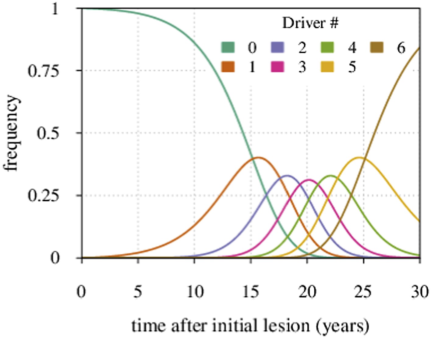
Maximal tumour heterogeneity in terms of driver subclones occurs at intermediate times after initial lesion.
https://doi.org/10.7554/eLife.06266.027
Appendix 1—figure 4
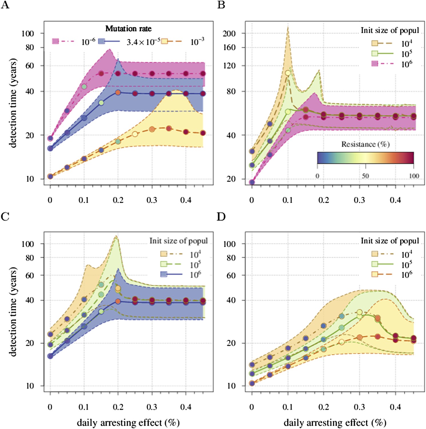
Sensitivity analysis of (A) the mutation rate to acquire drivers and (B–D) initial tumour size.
Thick lines indicate the median and shaded areas with dashed boundaries the 90% confidence intervals of detection times. (A) Initial tumour size is fixed at 106 cells and mutation rate is varied. (B–D) Initial tumour size is varied and mutation rate is fixed at (B) 10−6, (C) 3.4 × 10⁻⁵, (D) 10−3. The colour code for points indicates the average level of resistance within tumours (see the inset in B). Parameter values as in Table 1 except those being varied.
Appendix 1—figure 5

Comparing the case shown in blue in Figure 2 with the case where resistant cells may become addicted to the drug.
The latter is illustrated by two treatment regimes: metronomic strategy (yellow) and constantly administrated drug (green). The plot shows the median and 90% confidence intervals (shaded areas) of detection times. The inset presents the fraction of cases when the tumour goes extinct after the initial lesion of 106 cells. Parameters as in Table 1.
Videos
Video 1
Treatment level affects both detection time and frequency of resistance.
(A) The median (thick line) and 90% confidence intervals (shaded areas with dashed boundaries) for the distribution of detection times. (B) Arbitrary samples of the distribution of detection times and distribution of the mean number of accumulated drivers. The colour-code indicates the average level of resistance in detected tumours over 3 month intervals. Parameters as in Table 1.
Video 2
Treatment level affects both detection time and frequency of resistance.
(A) The median (thick line) and 90% confidence intervals (shaded areas with dashed boundaries) for the distribution of detection times. (B) Arbitrary samples of the distribution of detection times and distribution of the mean number of accumulated drivers. The colour-code indicates the average level of resistance in detected tumours over 3 month intervals. Parameters as in Table 1 except for the cost of resistance c = 0.4%.
Video 3
Treatment level effects on detection times assuming no resistance is possible.
(A) The median (thick line) and 90% confidence intervals (shaded areas with dashed boundaries) for the distribution of detection times. (B) Arbitrary samples of the distribution of detection times and the distribution of the mean number of accumulated drivers. The colour-code indicates the average level of resistance in detected tumours over 3 month intervals. The resistance mutation is knocked out (v = 0). Otherwise parameters as in Table 1.
Video 4
Comparison of preventive (blue lines and shading) and post-diagnostic (red lines, hatched) interventions.
Tumours are treated at M0 = 106 cells. (A) The median (thick line) and 90% confidence intervals (shaded areas with dashed boundaries) for the distribution of times to relapse for treatment failures. (B) and (C) Arbitrary samples of the distribution of detection times for preventive and post-diagnostic interventions, respectively. The colour-code indicates the mean number of accumulated drivers over a period of 1 year. The rectangles on the top of B and on the bottom of C show the fifth and 95th percentiles, the blue circle indicates the median, and the red line is the mean. Parameters as in Table 1.
Video 5
Comparison of preventive (blue lines and shading) and post-diagnostic (red lines, hatched) interventions.
Tumours are treated at M0 = 104 cells. (A) The median (thick line) and 90% confidence intervals (shaded areas with dashed boundaries) for the distribution of times to relapse for treatment failures. (B) and (C) Arbitrary samples of the distribution of detection times for preventive and post-diagnostic interventions, respectively. The colour-code indicates the mean number of accumulated drivers over a period of 1 year. The rectangles at the top of B and the bottom of C shows the fifth and 95th percentiles, the blue circle indicates the median, and the red line is the mean. Parameters as in Table 1.
Tables
Table 1
Baseline parameter values used in this study
| Parameter | Variable | Value | Range | Ref. |
|---|---|---|---|---|
| Time step (cell cycle length) | T | 4 days | 3–4 days | (Bozic et al., 2010) |
| Selective advantage | s | 0.4% | 0.1–1.0% | (Bozic et al., 2010) |
| Cost of resistance | c | 0.1% | ||
| Mutation rate to acquire an additional driver | u | 3.4 × 10⁻⁵ | 10−7–10−2 | (Bozic et al., 2010) |
| Mutation rate to acquire resistance | v | 10−6 | 10−7–10−2 | (Komarova and Wodarz, 2005) |
| Maximal number of additional drivers | N | 5 (Figures 1, 2) 9 (other figures) | 0–9 | |
| Initial cell population | M0 | 106 cells | – | |
| Pre-resistance level | κ | 0.01% | – | (Iwasa et al., 2006) |
| Number of replicate numerical simulations (excluding extinctions) | – | 106 | – | |
| Detection threshold | M | 109 cells | 107–1011 | (Beckman et al., 2012) |
-
‘Range’ is values from previous study and employed in the present study.
Download links
A two-part list of links to download the article, or parts of the article, in various formats.
Downloads (link to download the article as PDF)
Open citations (links to open the citations from this article in various online reference manager services)
Cite this article (links to download the citations from this article in formats compatible with various reference manager tools)
Dynamics of preventive vs post-diagnostic cancer control using low-impact measures
eLife 4:e06266.
https://doi.org/10.7554/eLife.06266


