Three ancient hormonal cues co-ordinate shoot branching in a moss
- University of Cambridge, United Kingdom
- Umeå University, Sweden
- Palacký University and Institute of Experimental Botany ASCR, Czech Republic
Figures
Figure 1
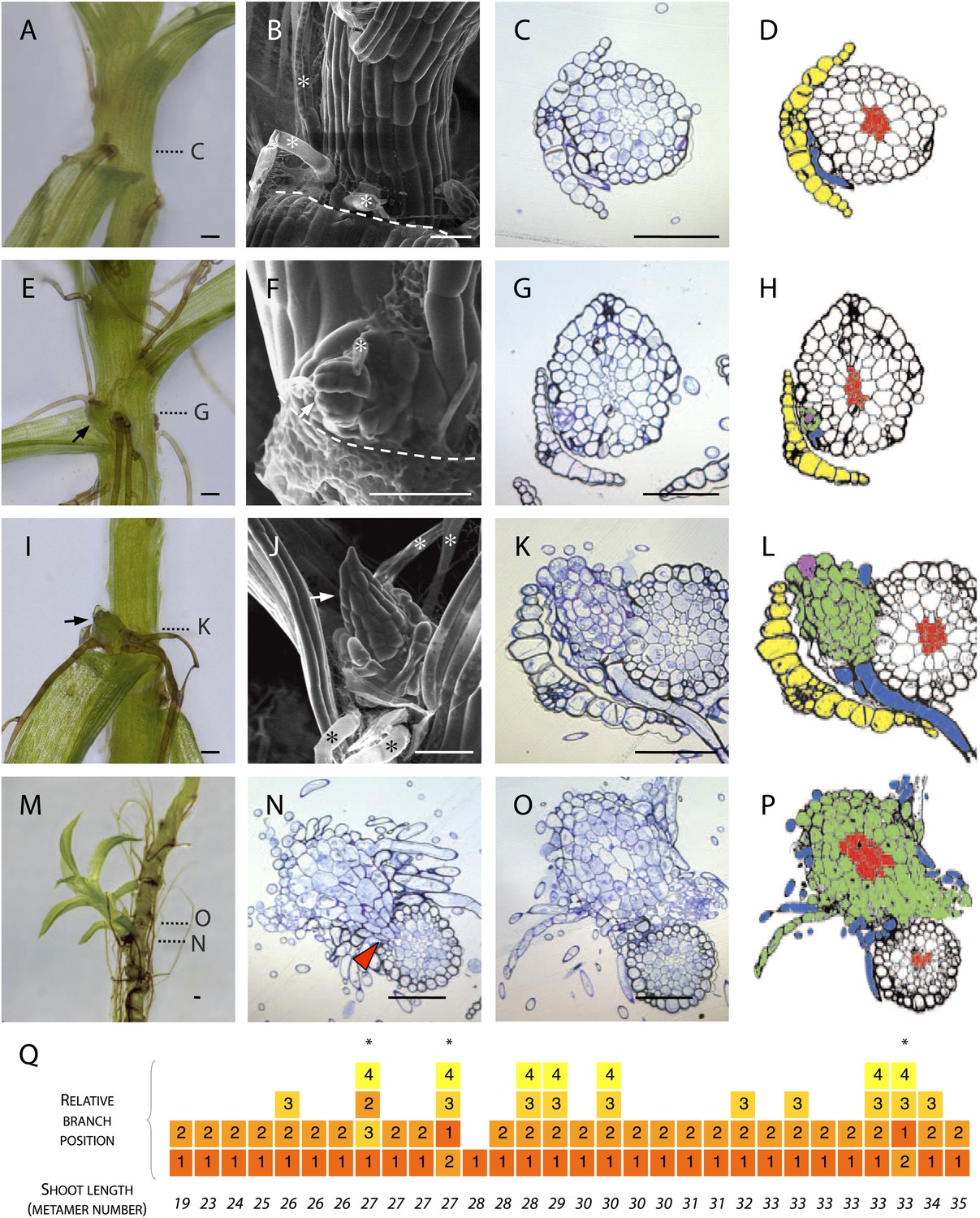
Branches initiate from the epidermis or outermost cortical cell layer in Physcomitrella.
(A–D) Although all leaf axils contained axillary rhizoids, branches were absent in most. (A) Light micrograph, (B) scanning electron microscope (SEM) micrograph, (C) transverse histological section and (D) corresponding line drawing showing a rhizoid (blue) in the axil of a leaf (yellow). Gametophore conducting tissues are shown in red. The label C in (A) indicates the approximate plane of section in (C). (E–H) At the earliest detectable stage of branching, each branch comprised a single apical cell surrounded by leaf initials and was adjacent to one or several developing rhizoids. (E) Light micrograph, (F) SEM micrograph, (G) transverse histological section and (H) corresponding line drawing showing a branch apical cell (pink) surrounded by leaf initials (green) and adjacent to an initiating rhizoid (blue). The label G in (E) indicates the approximate plane of section in (G). (I–L) At a later stage, growing buds had well-developed leaves. (I) Light micrograph, (J) SEM micrograph, (K) transverse histological section and (L) corresponding line drawing showing a well-developed bud (green) and its apical cell (pink) in the axil of the leaf (yellow). The label K in (I) indicates the approximate plane of section in (K). (M–P) Well-developed branches persisted as superficial projections, there was no continuity between the conducting tissue system of the branch and the gametophore axis. (M) Light micrograph of a lateral branch on a gametophore whose leaves have been removed. (N) Transverse histological section at the junction point of the lateral branch with the main gametophore axis (indicated by N in [M]), the red arrowhead shows cortical tissue and the absence of continuity between conducting tissue systems. (O) Transverse histological section and (P) corresponding line drawing above the junction point (indicated by O in [M]) where the conducting tissues (red) of the lateral branch (green) and the main axis (white) can be seen. (Q) The sequence of branch initiation in thirty 6 week old gametophores. For all images, arrows show lateral buds, dotted lines indicate the level of corresponding histological sections, asterisks mark rhizoids, dashed lines mark the boundary between the stem and the detached leaf. Scale bars = 100 μm.
Figure 2 with 2 supplements

Branching patterns are non-random.
(A) A wild-type gametophore before (left) and after (right) removing the leaves. Asterisks indicate lateral branches. Scale bar = 1 mm. (B) Each gametophore is represented as 1-D series of metamers (light green squares) and lateral branch position is indicated in dark green. (C–E) Branching patterns of 60 gametophores ordered by increasing size showing the apical inhibition zone (AIZ) and branching zone (BZ). Data from wild-type (C), stochastic simulation (D) and stochastic simulation with imposed apical inhibition (E) had similar branch numbers but different branch distributions. (F–I) Assumptions and replacement rules of the computational model. (F) Each gametophore starts off as an apex (red), which produces auxin and grows by producing metamers (grey) containing auxin at concentration c. (G) illustrates replacement rules used in simulations. 1: an apex (red) regularly produces metamers (grey). 2: if auxin concentration c in a metamer falls below the auxin sensitivity threshold T, then the metamer becomes a branch and an auxin source (red). 3: if auxin concentration c is higher than T, then branch formation is inhibited. (H) The auxin concentration c within a metamer reflects acropetal transport defined by the constant KA and basipetal transport defined by the constant KB. (I) Stages of growth in a single simulated gametophore showing that, as new metamers are added, the ratio of c/T drops towards the base, allowing a branch to initiate (compare iii to iv). The new apex becomes an auxin source and can export auxin both up and down the gametophore (v). This results in the formation of an auxin minimum further up the gametophore axis and a second branch initiates (vi to vii).
Figure 2—figure supplement 1
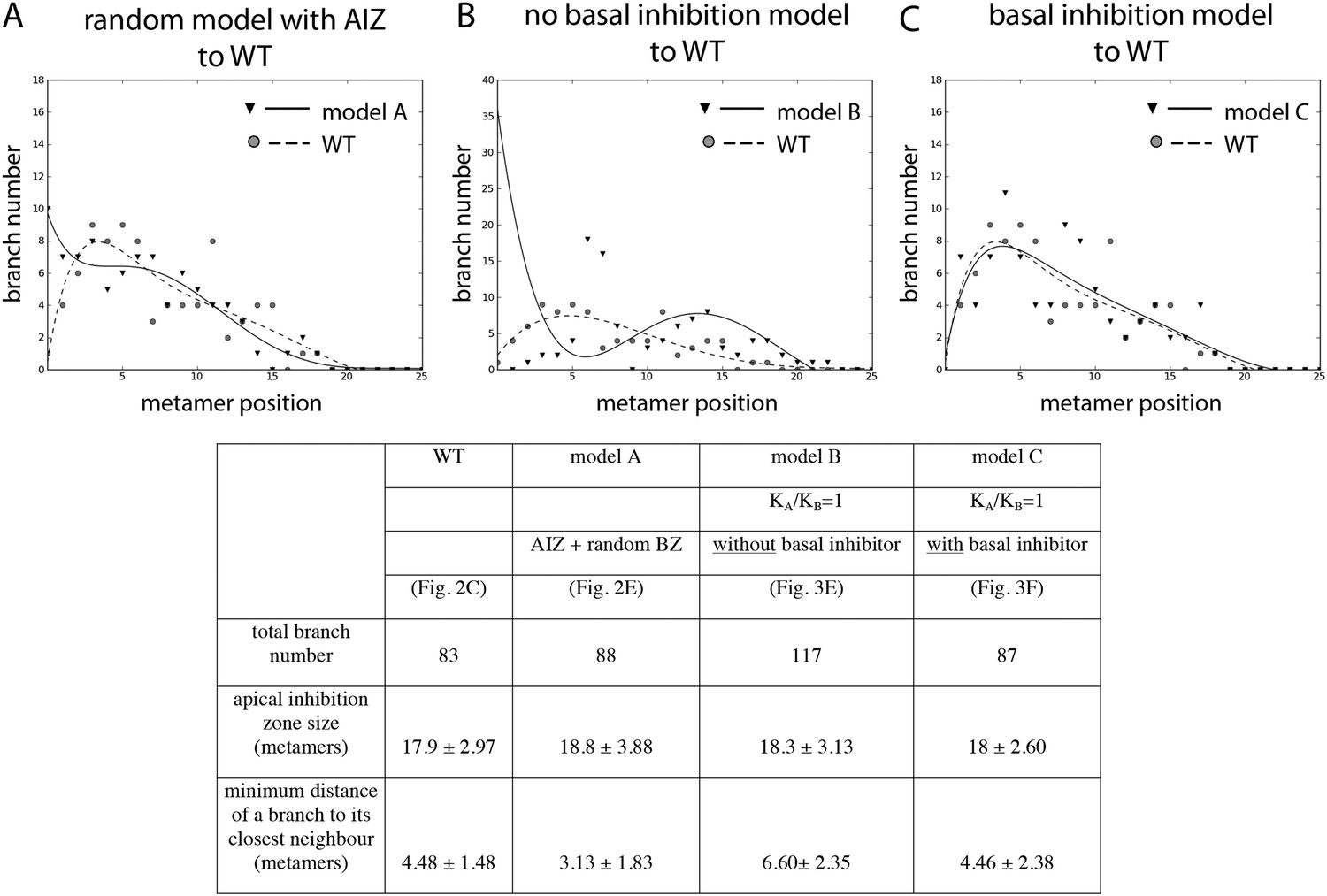
Comparison of the WT branching pattern plot with different model outputs.
(A–C) Model C (directionally unbiased transport, with basal inhibitor) best approximates the distribution of branches observed in WT. Model A, in which an apical inhibition zone is specified to match WT but there is a random branch distribution in the branching zone, does not capture WT branch distribution. Model B, in which there is no basal inhibitor and transport is directionally unbiased, shows a shift in branch distribution due to the constitutive basal activation. Lines indicate the best fitting polynomial of the seventh degree. For model B, a polynomial of the fifth degree was selected to fit the data points. Table: comparison of WT branching patterns to different model outputs. Model C is the best fit to WT branch number, apical inhibition zone size and minimum distance of a branch to its closest neighbour in comparison to models A and B.
Figure 2—figure supplement 2

Stages of growth in a single simulated gametophore showing that as new metamers are added, the ratio of c/T drops towards the base, allowing a branch to initiate (compare v to vi).
The new apex becomes an auxin source and can export auxin both up and down the gametophore (vi). This results in the formation of an auxin minimum further up the gametophore axis and a second branch initiates (vii, A). The zone of basal inhibition is indicated by green metamer outlines (B). Minima of c/T can initiate out of acropetal series (C).
Figure 3
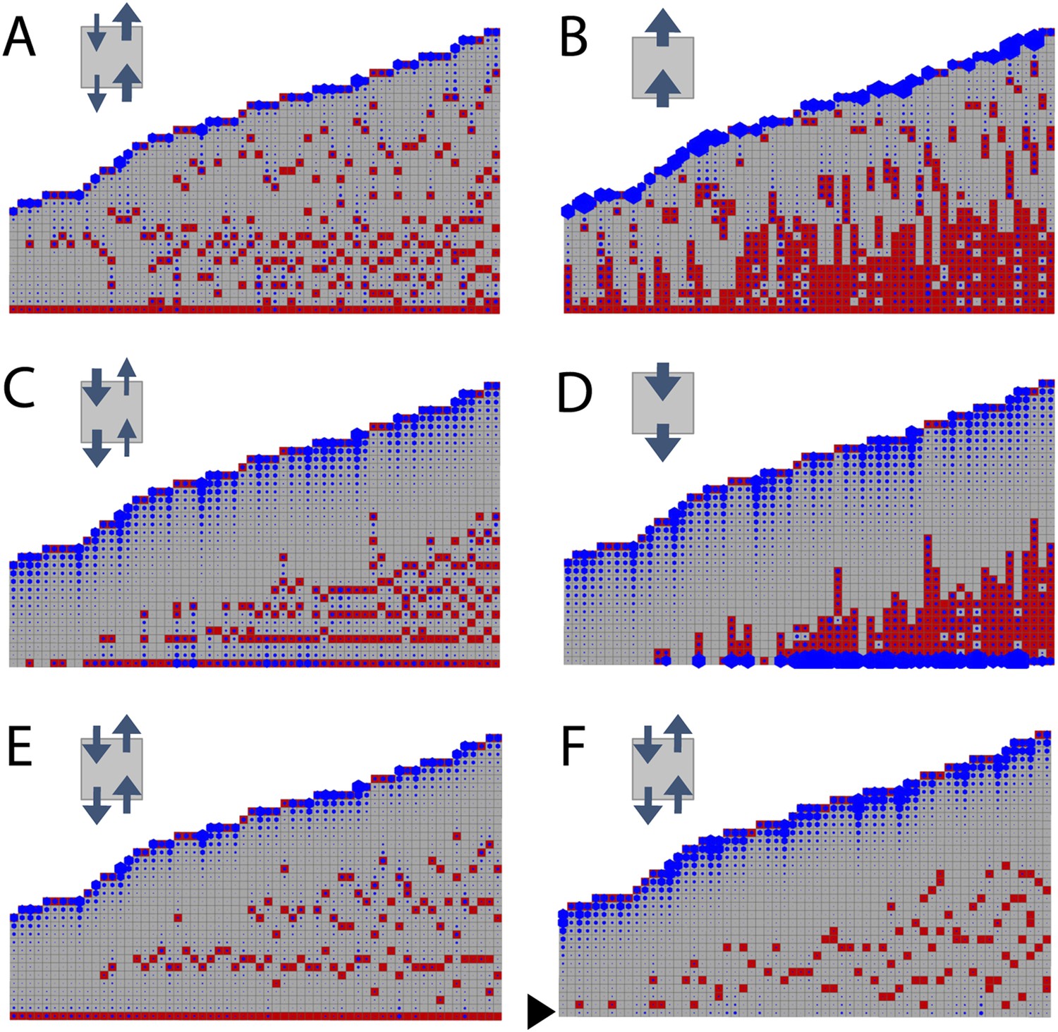
Simulated branching patterns are sensitive to changes in the direction of auxin transport and predict a basal branching inhibitor.
(A–B) Output of simulations with mainly acropetal auxin transport, set to KA/KB = 3 (A) or KA/KB = 100 (B). (C–D) Output of simulations with predominantly basipetal transport, set to KA/KB = 1/3 (C) or KA/KB = 1/100 (D). (E, F) Output of simulations with bi-directional auxin transport set to KA/KB = 1. Without local basal reduction of the branching threshold (T, black arrow), the most basal metamer always produced a branch (E). A reduction of the branching threshold in the basal metamers was required to generate a realistic WT branching pattern (F). For all insets, arrow sizes indicate the relative amount of basipetal and acropetal auxin transport. Red indicates gametophore and branch apices, and blue indicates the auxin concentration (c) relative to T.
Figure 4
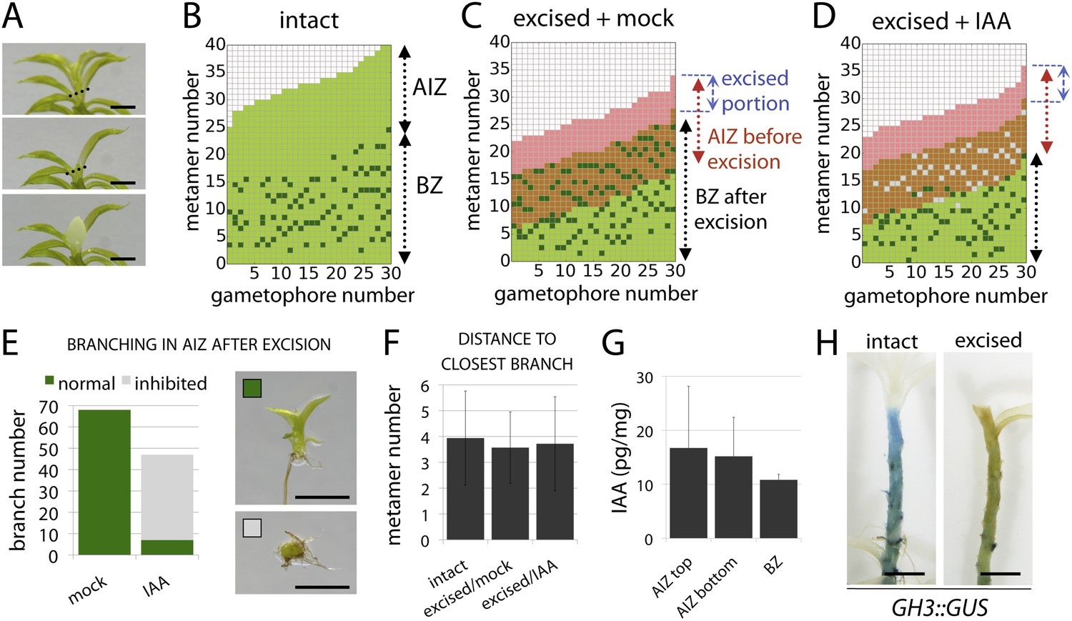
The main Physcomitrella gametophore apex is an auxin source that suppresses branching.
(A) Gametophores were isolated from wild-type colonies (top), and the six top metamers were excised at the dotted line (middle) and replaced with lanolin or lanolin plus 1 mM auxin (bottom). Scale bar = 1 mm. (B) Branching pattern of 30 intact gametophores ordered by increasing size. AIZ, apical inhibition zone. BZ, branching zone. (C) Branching pattern of 30 gametophores 5 days after excision. Lateral branches activated in the portion of gametophore corresponding to the apical inhibition zone before excision, coloured in red. (D) Branching pattern of 30 gametophores 5 days after excision and replacement of the apex by a source of auxin. (E) The number of normal and defective branches formed in the apical inhibition zone of mock and IAA-treated gametophores. (F) Mean minimum metamer number between lateral branches was not affected by gametophore apex excision. (G) shows mean auxin levels quantified from five biological replicates; levels were are highest at the tip of the gametophore and decreased toward the base. (H) GH3::GUS expression was high in the apical inhibition zone (left) and was strongly reduced after decapitation (right). Scale bar = 1 mm.
Figure 5

Globally applied exogenous auxins inhibit branch initiation.
(A–D) Branching patterns in wild-type gametophores grown for 5 weeks, immersed for 24 hr in mock (A), 1 μM IAA (B), 100 nM NAA (C) or 1 μM 2,4-D (D) and grown for another 2 weeks. (E–H) mock (E), IAA (F), NAA (G) and 2,4-D (H) treated gametophores before (left) and after (right) removing the leaves, with asterisks indicating lateral branches. Scale bar = 1 mm. (I–K) Bubble plots showed that branch number decreased in response to IAA (I), NAA (J) and 2,4-D (K) compared with mock-treated gametophores. Gametophore length is depicted as the number of metamers and the bubble area is proportional to the number of gametophores with a similar branch number at a particular length. Ordinary least squares regression was used to test whether the relationship between branch number and gametophore leaf number depended on treatment (see ‘Material and methods’), and for (I) the best fitting model was B = (−4.45 + 2.52X) + (0.2 − 0.12X)L meaning that IAA treatment significantly differed from mock treatment (p < 0.01). For (J) the best fitting model was B = (−4.45 + 2.87X) + (0.2 − 0.13X)L; NAA treatment significantly differed from mock treatment (p < 0.001). For (K) the best fitting model was B = (−4.45 + 2.8X) + (0.2 − 0.13X)L; 2,4-D treatment significantly differed from mock treatment (p < 0.001). (L) The apical inhibition zone size increased in response to IAA, NAA and 2,4-D (mean ± SD; bilateral t-test different from mock control, *p < 0.05).
Figure 6 with 1 supplement

Auxin biosynthesis mutants and transgenics match predicted effects of changing parameter values of Hapex and H.
(A–B) Model simulations of branching patterns with Hapex and H values reduced from 80 ± 20 to 48 ± 12 and from 20 ± 4.5 to 12 ± 2.7 respectively (A) or Hapex and H values increased from 80 ± 20 to 240 ± 60 and from 20 ± 4.5 to 60 ± 13.5 (B). (C–D) Branching patterns in shi2-1 mutants with reduced auxin biosynthesis levels (C) and SHI ox-5 transgenics with elevated auxin biosynthesis levels (D). (E–F) shi2-1 (E) and SHI ox-5 (F) gametophores before (left) and after (right) removing the leaves, with asterisks indicating lateral branches. Scale bar = 1 mm. (G–H) Bubble plots showed that branch number increased in shi2-1 (G) and diminished in SHI ox-5 (H) compared with WT gametophores. Gametophore length is depicted as the number of metamers and the bubble area is proportional to the number of gametophores with a similar branch number at a particular length. For (G) the best fitting model was B = (−3.27 + 1.16X) + 0.18L; shi2-1 significantly differed from WT (p < 0.001). For (H) the best fitting model was B = (−3.29 + 2.05X) + (0.18 − 0.11X)L, SHI ox-5 significantly differed from WT (p < 0.001). (I) Apical inhibition zone size was reduced in shi2-1 and increased in SHI ox-5 (mean ± SD; bilateral t-test different from WT, *p < 0.05). (J) Minimum distance between lateral branches was reduced in shi2-1 (mean ± SD; bilateral t-test different from WT, *p < 0.05). n.d., not determined because branch number was insufficient.
Figure 6—figure supplement 1
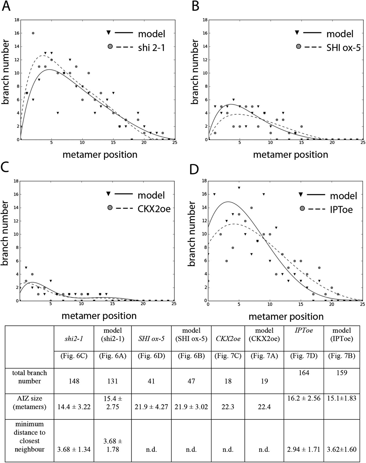
Comparison of mutant branching pattern plots with model outputs.
Every model closely approximates the branch distribution as a function of metamer position, the total branch number, the apical inhibition zone size and the minimum distance of a branch to its closest neighbour for every corresponding mutant. n.d., not determined because branch number was insufficient. Table: comparison of mutant branching patterns with model outputs.
Figure 7 with 1 supplement

Cytokinin biosynthesis mutants and transgenics match predicted effects of changing parameter values of T and exogenous cytokinin treatment is sufficient for lateral meristem formation.
(A) Model simulation of branching patterns with T values reduced from 3 ± 0.8 to 0.45 ± 0.2. (B) Model simulation of branching patterns with T values increased from 3 ± 0.8 to 5.4 ± 0.8. (C–D) Branching patterns in CKX2oe transgenics with reduced cytokinin levels (C) and IPToe transgenics with increased cytokinin levels (D). (E–F) CKX2oe (E) and IPToe (F) gametophores before (left) and after (right) removing the leaves, with asterisks indicating lateral branches. Scale bar = 1 mm. (G–H) Bubble plots showed that branch number diminished in CKX2oe (G) and increased in IPToe (H) compared with WT gametophores. Gametophore length is depicted as the number of metamers and the bubble area is proportional to the number of gametophores with a similar branch number at a particular length. (G) The best fitting model was B = (−3.28 + 3.19X) + (0.18 − 0.17X)L, CKX2oe significantly differed from WT (p < 0.001). (H) The best fitting model was B = (−3.69 + 1.28X) + 0.2L, IPToe significantly differed from WT (p < 0.001). (I) Apical inhibition zone size was reduced in IPT1oe (mean ± SD; bilateral t-test different from WT, *p < 0.05). (J) Minimum distance between lateral branches was reduced in IPT1oe (mean ± SD; bilateral t-test different from WT, *p < 0.05). n.d., not determined because branch number was insufficient. (K–N) Exogenous cytokinin treatment promoted branch initiation. WT gametophores 1 week after immersion in mock (K) or 1 μM BAP (L) solution for 24 hr. Cytokinin promoted development of callus-like structures (M). Scale bar = 1 mm. (N) Confocal microscope image showing that cytokinin-induced structures were mainly constituted of leaves (white asterisks) resulting from the proliferation of ectopic meristematic cells. Scale bar = 100 μm.
Figure 7—figure supplement 1
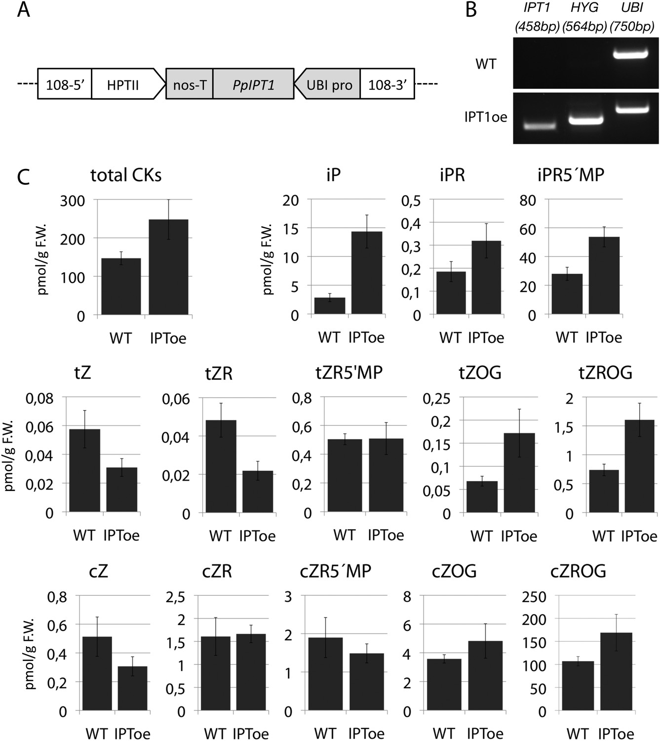
Molecular characterization and cytokinin profiling of the PpIPT1 overexpressing line.
(A) Schematic of the genetic construct pTHUBI-PpIPT1 (modified from pTHUBI-Gateway [Perroud et al., 2011]). Used to generate PpIPT1 overexpressing lines. (B) RT-PCR analysis detected strong expression of PpIPT1 and HYG genes in wild-type plants genetically transformed with pTHUBI-PpIPT1 (IPToe), but not in untransformed wild-type plants (WT). PpUBI gene was used as internal control. (C) Cytokinin (CK) profiling showed a global increase in CK levels in IPToe transgenics in comparison with WT. CK levels represent the mean (± s.d.) of four biological replicates and are expressed in pmol per gram of fresh weight (pmol/g F.W.). iP, N-isopentenyladenine; iPR, N-isopentenyladenosine; iPR5′MP, N-isopentenyladenosine-5′-monophosphate; tZ, trans-zeatin; tZR, trans-zeatin riboside; tZR5′MP, trans-zeatin riboside-5′-monophosphate; tZOG, trans-zeatin O-glucoside; tZROG, trans-zeatin riboside O-glucoside; cZ, cis-zeatin; cZR, cis-zeatin riboside; cZR5′MP, cis-zeatin riboside-5′-monophosphate; cZOG, cis-zeatin O-glucoside; cZROG, cis-zeatin riboside O-glucoside.
Figure 8

PIN-mediated auxin transport is a minor contributor to branching patterns.
(A–D) Branching patterns in GH3::GUS, pina, pinb and pina pinb mutants. (E–H) GH3::GUS (E), pina (F), pinb (G) and pina pinb (H) gametophores before (left) and after (right) removing leaves, with asterisks indicating lateral branches. Scale bar = 1 mm. (I) Apical inhibition zone size is significantly reduced in the pina pinb double mutant but not in pina or pinb single mutants (mean ± SD; bilateral t-test different from GH3::GUS, *p < 0.05). (J–L) Bubble plots showed that branch number increases in pinb (K) and pina pinb (L) but not pina (J) compared with GH3::GUS gametophores. Gametophore length is depicted as the number of metamers and the bubble area is proportional to the number of gametophores with a similar branch number at a particular length. The best fitting model for (J) was B = −2.8 + 0.15L, pina was not significantly different from GH3::GUS. The best fitting model for (K) was B = (−2.47 − 1.40X) + (0.14 + 0.07X)L, pinb was significantly different from GH3::GUS (p < 0.01). The best fitting model for (L) was B = (−2.96 + 0.52X) + 0.15L, pina pinb significantly differed from GH3::GUS (p < 0.01). (M) The minimum distance between lateral branches is reduced in pina, pinb and pina pinb mutants with respect to GH3::GUS controls (mean ± SD; bilateral t-test different from GH3::GUS, *p < 0.05), thus branch density in the branching zone is higher in all the mutants. (N–O) Branching patterns in GH3::GUS mutants treated without (N) or with (O) 5 μM NPA. (P–R) 5 μM NPA treatment did not affect the branch number in GH3::GUS transgenics (P), the apical inhibition zone size (Q) and the minimum distance between lateral branches (R). For (P), the best fitting model was B = −3.64 + 0.2L; NPA treatment was not significantly different from the mock treatment. (S–T) Branching patterns in pina pinb mutants treated without (S) or with (T) 5 μM NPA. (U–W) 5 μM NPA treatment did not affect the branch number in pina pinb mutants (U), the apical inhibition zone size (V) and the minimum distance between lateral branches (W). For (U), the best fitting model was B = −1.99 + 0.14L; NPA treatment was not significantly different from the mock treatment. (X–Y) Branching patterns in WT treated without (X) or with (Y) 5 μM BUM. (Z–AB) 5 μM BUM treatment did not affect the branch number in WT (Z), the apical inhibition zone size (AA) and the minimum distance between lateral branches (AB) (mean ± SD). For (Z), the best fitting model was B = −1.24 + 0.07L; BUM treatment was not significantly different from the mock treatment.
Figure 9 with 1 supplement
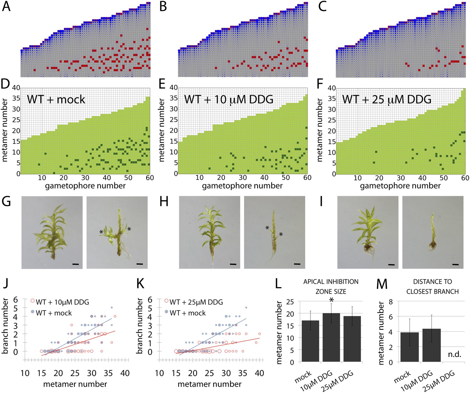
A callose synthesis inhibitor regulates branching.
(A–C) Model simulation of branching patterns with K values increased from 0.025 (A) to 0.045 (B) and 0.07 (C). (D–F) Branching patterns in wild-type gametophores treated with mock (D), 10 μM 2-deoxy-glucose (DDG) (E) or 25 μM DDG (F). (G–I) mock (G), 10 μM DDG (H) or 25 μM DDG (I) treated gametophores before (left) and after (right) removing the leaves, with asterisks indicating lateral branches. Scale bar = 1 mm. (J–K) Bubble plots show that branch number diminishes in 10 μM DDG (J) and is strongly reduced in 25 μM DDG (K) treated gametophores compared with mock treatment. Gametophore length is depicted as the number of metamers and the bubble area is proportional to the number of gametophores with a similar branch number at a particular length. The best fitting model for (J) was B = (−3.82 + 1.41X) + (0.21 − 0.08X)L, 10 μM DDG was significantly different from mock treatment (p < 0.001). The best fitting model for (K) was B = (−3.82 + 2.47X) + (0.21 − 0.14X)L, 25 μM DDG was significantly different from mock treatment (p < 0.001). (L) Apical inhibition size is significantly increased in response to DDG treatment (mean ± SD; bilateral t-test different from WT mock, *p < 0.05). (M) The minimum distance between lateral branches is not different in 10 μM DDG treated gametophores with respect to mock controls (mean ± SD). n.d., not determined because branch number was insufficient.
Figure 9—figure supplement 1
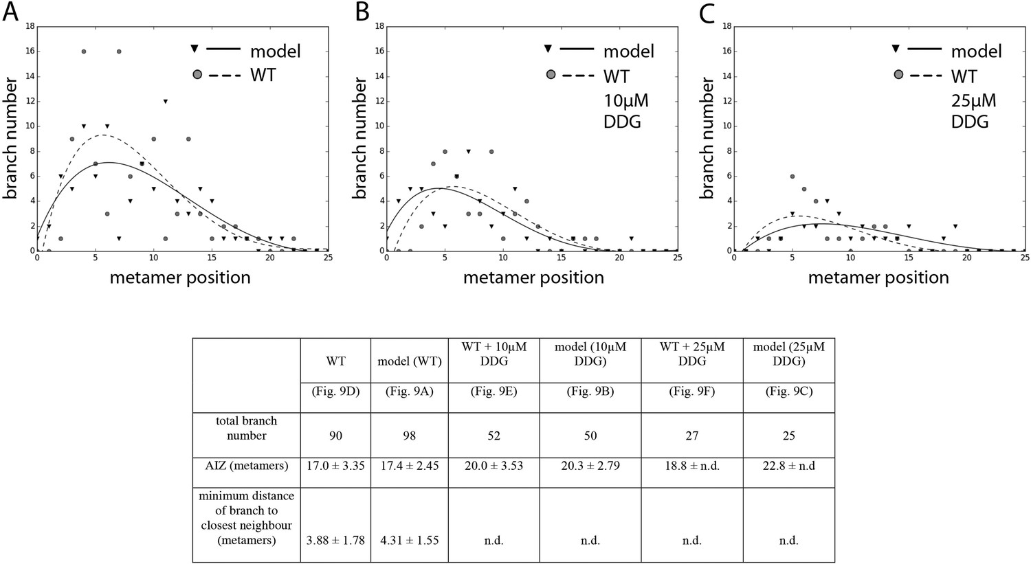
Comparison of branching pattern plots from pharmacologically treated plants with model outputs.
Every model closely approximates the branch distribution as a function of metamer position, the total branch number, the apical inhibition zone size and the minimum distance of a branch to its closest neighbour for every corresponding mutant. n.d., not determined because branch number was insufficient. Table: comparison of branching patterns from pharmacologically treated plants with model outputs'.
Figure 10 with 1 supplement
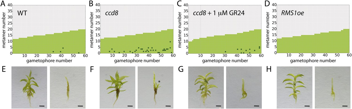
Expression levels of a strigolactone biosynthesis gene modulates branching.
(A–D) Branching patterns of 60 gametophores with fewer than 20 leaves in (A) WT, (B) strigolactone-deficient ppccd8 mutants, (C) ppccd8 mutants treated with 1 μM GR24 and (D) RMS1oe transgenics with increased strigolactone levels. (E–H) WT (E), ppccd8 (F), GR24-treated ppccd8 (G) and RMS1oe (H) gametophores before (left) and after (right) removing the leaves, with asterisks indicating lateral branches. Scale bar = 1 mm.
Figure 10—figure supplement 1
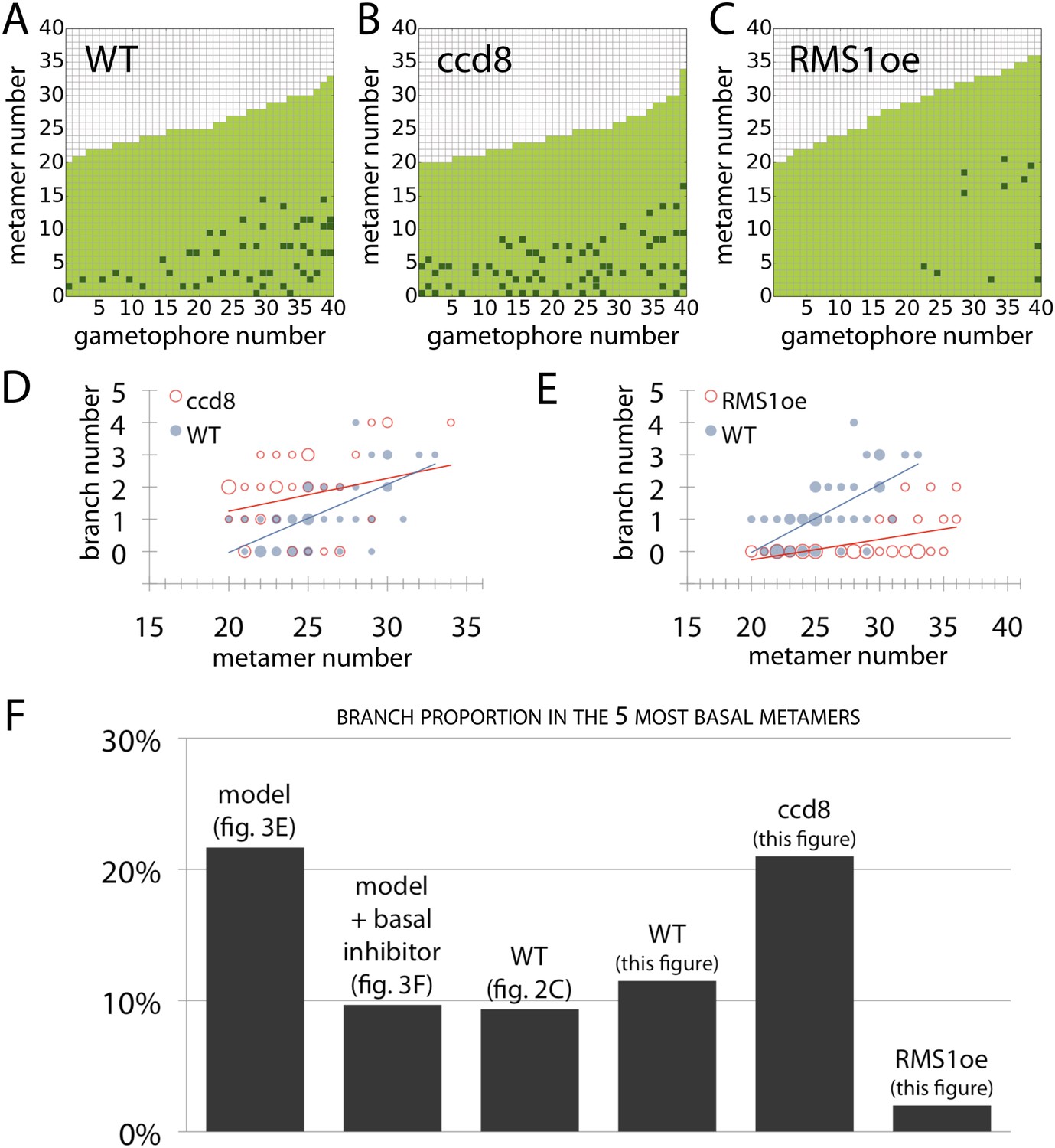
Branching patterns of gametophores with more than 20 leaves and branch proportion in the five most basal metamers.
(A–C) Branching patterns of 40 gametophores with more than 20 leaves in (A) WT, (B) strigolactone-deficient ppccd8 mutants and (C) RMS1oe transgenic lines with increased strigolactone levels. (D–E) Bubble plots show that branch number increases at the base of ccd8 mutants (D) and is strongly reduced in RMS1oe transgenics (E) compared with WT gametophores. Gametophore length is depicted as the number of metamers and the bubble area is proportional to the number of gametophores with a similar branch number at a particular length. The best fitting model for (D) was B = (−2.84 + 0.73X) + 0.16L, ccd8 was significantly different from WT (p < 0.01). The best fitting model for (E) was B = (−4.25 + 2.71X) + (0.21 − 0.15X)L, RMS1oe was significantly different from WT (p < 0.001). (F) Branch proportion in the five most basal metamers is similar between the ‘no basal branching inhibitor’ model output (Figure 3E) and ppccd8 mutants (B, D). Addition of a basal branching inhibitor in the model simulations (Figure 3F) captures basal branch proportion of WT gametophores (A, Figure 2C). Increase of strigolactone biosynthesis suppresses basal branching in RMS1oe gametophores (C, E).
Videos
Video 1
(corresponds to Figure 3A) Simulation of branching activation pattern with mainly acropetal auxin transport (set to KA/KB = 3) and no basal branching inhibitor.
https://doi.org/10.7554/eLife.06808.010
Video 2
(corresponds to Figure 3B) Simulation of branching activation pattern with mainly acropetal auxin transport (set to KA/KB = 100) and no basal branching inhibitor.
https://doi.org/10.7554/eLife.06808.011
Video 3
(corresponds to Figure 3C) Simulation of branching activation pattern with mainly basipetal auxin transport (set to KA/KB = 1/3) and no basal branching inhibitor.
https://doi.org/10.7554/eLife.06808.012
Video 4
(corresponds to Figure 3D) Simulation of branching activation pattern with mainly basipetal auxin transport (set to KA/KB = 1/100) and no basal branching inhibitor.
https://doi.org/10.7554/eLife.06808.013
Video 5
(corresponds to Figure 3E) Simulation of branching activation pattern with equal basipetal and acropetal auxin transport (set to KA/KB = 1) and no basal branching inhibitor.
https://doi.org/10.7554/eLife.06808.014
Video 6
(corresponds to Figure 3F) Simulation of branching activation pattern with equal basipetal and acropetal auxin transport (set to KA/KB = 1) and with basal branching inhibitor.
https://doi.org/10.7554/eLife.06808.018
Video 7
(corresponds to Figure 6A) Simulation of branching activation pattern in the shi2-1 mutant.
https://doi.org/10.7554/eLife.06808.021
Video 8
(corresponds to Figure 6B) Simulation of branching activation pattern in the SHI ox-5 transgenic line.
https://doi.org/10.7554/eLife.06808.022
Video 9
(corresponds to Figure 7A) Simulation of branching activation pattern in the CKX2oe transgenic line.
https://doi.org/10.7554/eLife.06808.025
Video 10
(corresponds to Figure 7B) Simulation of the branching activiation pattern in the IPT1oe transgenic line.
https://doi.org/10.7554/eLife.06808.026
Video 11
(corresponds to Figure 9A) Simulation of the WT branching activation pattern with refitted parameters.
https://doi.org/10.7554/eLife.06808.029
Video 12
(corresponds to Figure 9B) Simulation of branching activation pattern with K values increased by 100%.
https://doi.org/10.7554/eLife.06808.030
Video 13
(corresponds to Figure 9C) Simulation of branching activation pattern with K values increased by 200%.
https://doi.org/10.7554/eLife.06808.031Tables
Table 1
Parameter values for the models shown in Figures 3, 6, 7
| Model wild-type | Model shi2-1 | Model SHI ox-5 | Model CKX2oe | Model IPT1oe | |
|---|---|---|---|---|---|
| (Figure 3F) | (Figure 6A) | (Figure 6B) | (Figure 7A) | (Figure 7B) | |
| Hapex | µ = 80, σ = 20 | µ = 48, σ = 12 | µ = 240, σ = 60 | ||
| H | µ = 20, σ = 4.5 | µ = 12, σ = 2.7 | µ = 60, σ = 13.5 | ||
| T | µ = 3.0, σ = 0.8 | µ = 0.45, σ = 0.2 | µ = 5.4, σ = 0.8 | ||
| ν | 0.01 | ||||
| KA | 0.05 | ||||
| KB | 0.05 |
-
Parameter µ represents the mean and σ the variance of the normally distributed stochastic variables H and T. Parameter values left blank are identical to the wild-type model.
Table 2
Refitted parameter values for the models shown in Figure 9
Download links
A two-part list of links to download the article, or parts of the article, in various formats.
Downloads (link to download the article as PDF)
Open citations (links to open the citations from this article in various online reference manager services)
Cite this article (links to download the citations from this article in formats compatible with various reference manager tools)
Three ancient hormonal cues co-ordinate shoot branching in a moss
eLife 4:e06808.
https://doi.org/10.7554/eLife.06808


