A quantitative framework for whole-body coordination reveals specific deficits in freely walking ataxic mice
- Champalimaud Foundation, Portugal
Figures
Figure 1 with 1 supplement

LocoMouse system for analyzing mouse locomotor coordination.
(A) LocoMouse apparatus. The mouse walks freely across a glass corridor with mirror below at a 45° angle. A single high-speed camera captures side and bottom views at 400 fps. Infrared (IR) sensors trigger data collection. (B) Machine learning algorithms identify paws, nose and tail segments and track their movements in 3D. Example ‘paw’ and ‘not paw’ training images for SVM (Support Vector Machine) feature detectors are shown for side and bottom views. (C) Continuous tracks are obtained by post-processing the feature detections with a Multi-Target Tracking algorithm. (D) Continuous forward trajectories (x position vs time) for paws, nose, and tail. The inset illustrates the color code used throughout the paper to identify individual features. (E) Continuous vertical (z) trajectories of the two front paws. (F) Side-to-side (y) position of proximal (green) to distal (yellow) tail segments vs time. (G) Individual strides were divided into swing and stance phases for further analysis. Further validation of tracking algorithm is presented in Figure 1—figure supplement 1.
Figure 1—figure supplement 1

LocoMouse tracking validation.
(A) Comparison of manual (gray) and automated tracking (blue) for front left paw across 3 dimensions. From left to right, plots show normalized x, y, and z paw position aligned to stance onset (n = 43 strides from 9 movies of 3 mice). (B) Scatterplots of manual vs automated tracking positions (x, y, and z) for all frames (n = 4194) of the same 9 movies. Values where the difference between manual and automated tracking are larger than average paw size are color-coded in green. Correlation coefficients are Pearson's r. (C) Example tracking traces demonstrate that stride lengths can differ at similar walking speeds due to pauses in walking.
Figure 2 with 1 supplement
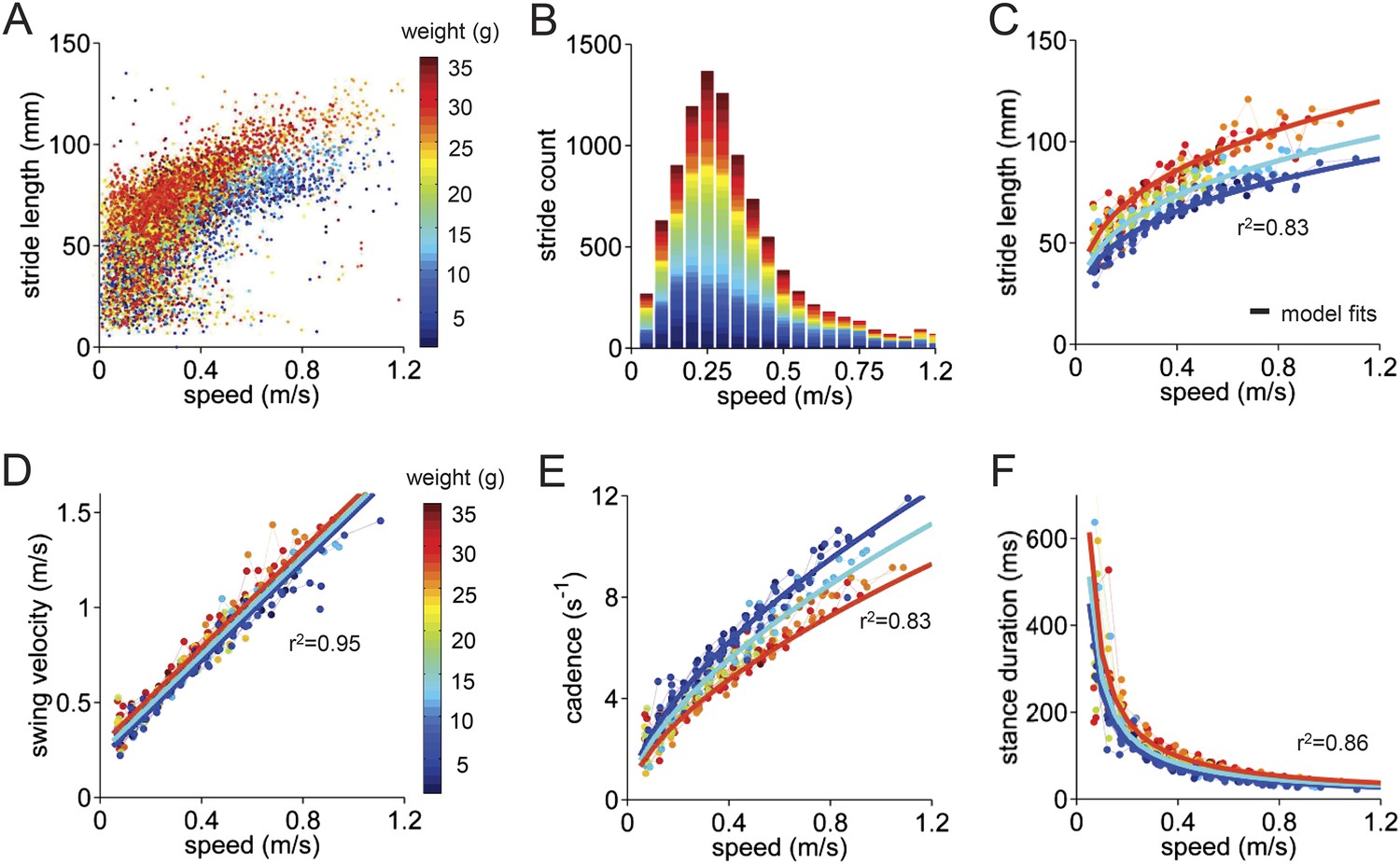
Basic stride parameters can be predicted using only walking speed and body size.
(A) Stride length vs walking speed for 9602 individual strides of the front right paws of 34 wildtype mice are color-coded by weight for each individual animal. More information on the mice can be found in Figure 2—figure supplement 1 and Figure 2—source data 1. (B) Histogram of average walking speeds for each stride from (A). Strides are divided into speed bins of 0.05 m/s. (C–F) Stride length, cadence (1/stride duration), swing velocity, and stance duration vs walking speed, respectively. For each parameter, speed-binned median values are shown for each animal (solid circles, color coded by weight). Data for each animal are connected across speeds with a thin dotted line. Thick lines are the output of the linear mixed-effects model, for 3 example weights across walking speeds (blue: 9g, cyan:19g, red: 33g). Marginal R-squared values for each linear mixed model are shown for each parameter. All raw data for Figure 2 and Figure 2—figure supplement 1 can be found in Figure 2—source data 1.
-
Figure 2—source data 1
Individual limb gait parameters, walking speed, and mouse metrics used to generate the linear mixed effects model in Figure 2.
Data for the four paws (FR HR FL HL) are stored in separate columns for all variables; rows are organized stride-wise. The linear mixed model shown in Figure 2 uses speed-binned data (0.05 m/s speed bins) from the FR paw, with a minimum stride count criterion of 5 strides per bin.
- https://doi.org/10.7554/eLife.07892.007
Figure 2—figure supplement 1
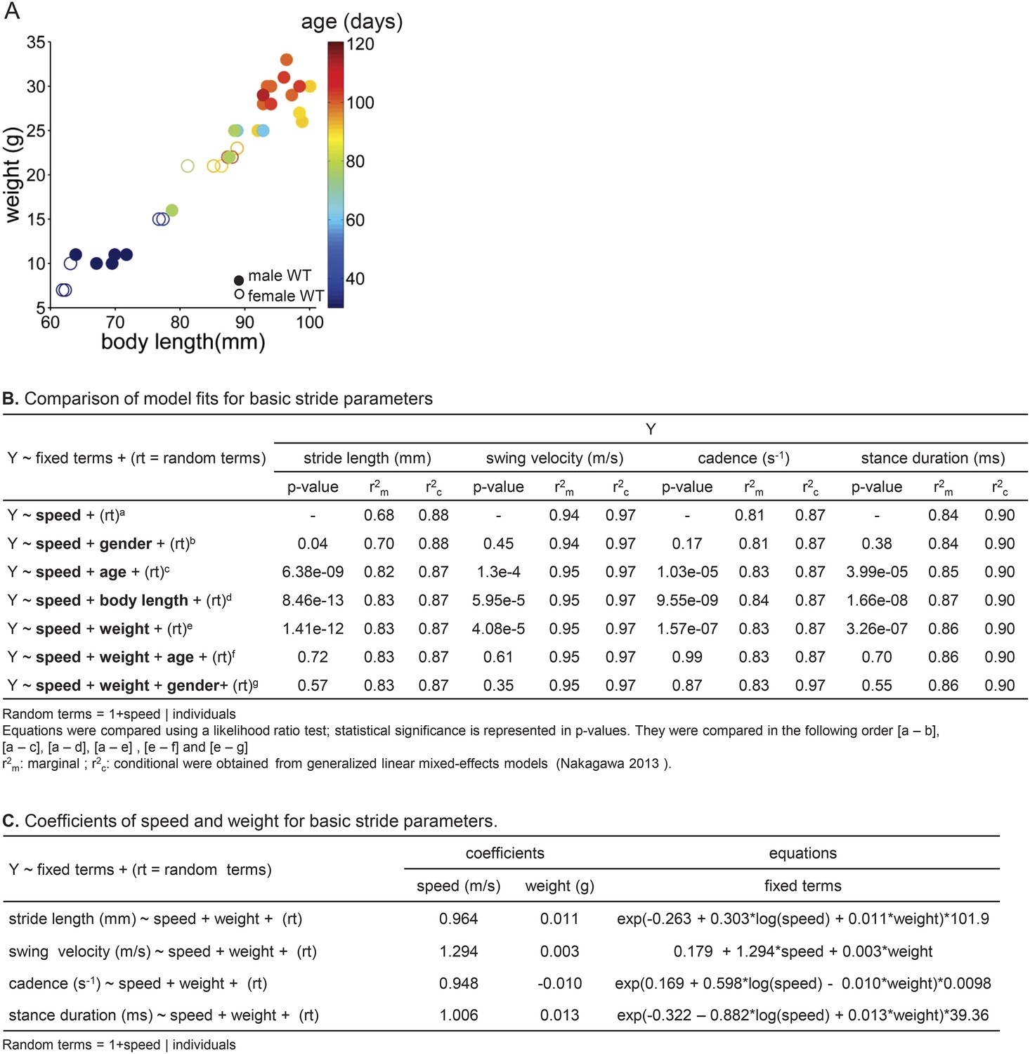
Using linear mixed effects models to predict basic stride parameters.
(A) Properties of wildtype mice used for linear mixed-effects model. A total of 34 wild-type C57BL/6 mice were used for the linear mixed-effects model in Figure 2. Each individual WT animal is plotted as a circle (open circles, females, N = 11; closed circles, males, N = 23). Symbols are color-coded by age. The diverse group included a variety of ages (30–114 days), body lengths (61–100 mm), and weights (7–33g). (B) Comparison of model fits for basic stride parameters. Speed, gender, age, body length, weight (fixed terms) and subject (random term) were used as predictor variables in the linear mixed-effects model. Table rows show tested equations for predicting stride parameters and values used for selection criteria of the resulting predictive model. p-values reported for each term are the outcome of a likelihood ratio test comparing indicated equations (superscripts). The last two lines (f, g) indicate that age and gender did not improve the predictions beyond the inclusion of speed and body weight. (C) Coefficients of speed and weight for basic stride parameters. The final equations for each stride parameter included speed and weight as fixed-term predictor variables; subject was included as a random-term. Coefficient values for fixed terms are represented. These equations can be used to predict stride parameters for a given mouse walking at a particular speed.
Figure 3 with 2 supplements
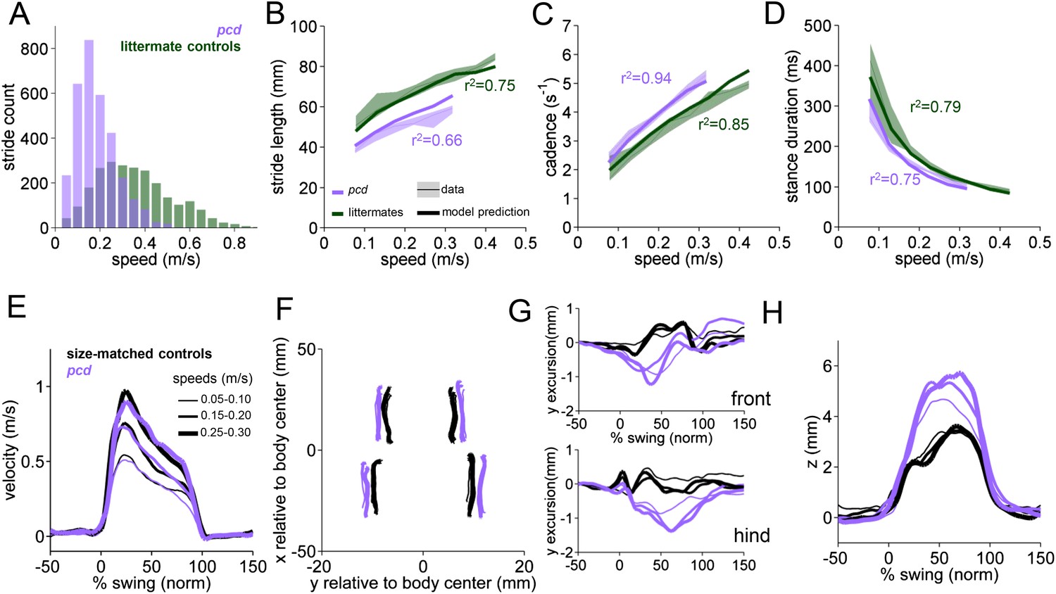
Differences in forward paw trajectories in pcd can be accounted for by walking speed and body size; impairments are restricted to off-axis movement.
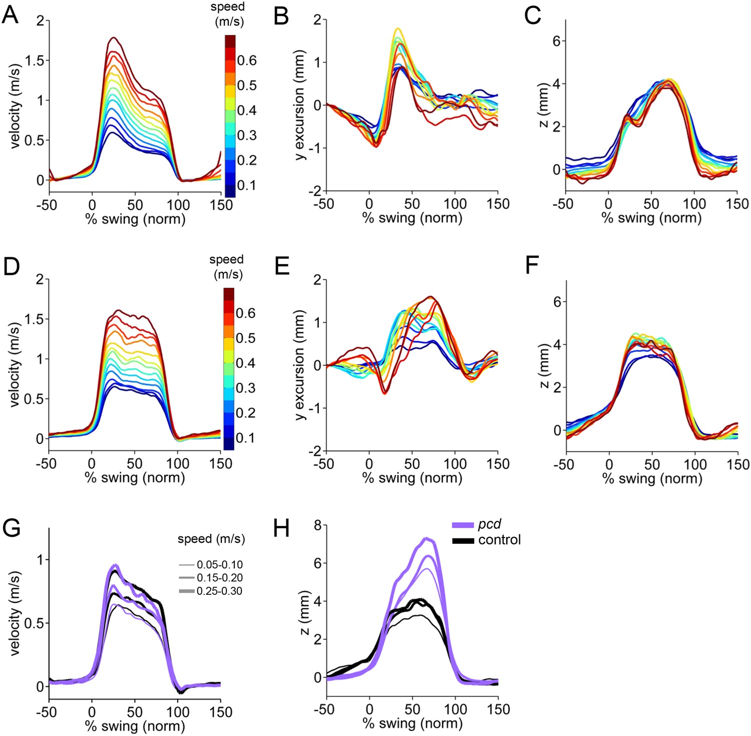
(A) Histogram of walking speeds, divided into 0.05 m/s speed bins for pcd (purple N = 3 mice; n = 3052 strides) and littermate controls (green, N = 7; n = 2256 strides). (B–D) Stride length (B), cadence (C, 1/stride duration) and stance duration (D) vs walking speed for pcd mice (purple) and littermate controls (green). For each parameter, the thin lines with shadows represent median values ±25th, 75th percentiles. Thick lines represent the predictions calculated using the mixed-effect models described in Figure 2 and Figure 2—figure supplement 1 (including speed and weight as predictor variables). (E) Average instantaneous forward (x) velocity of FR paw during swing phase for pcd (purple) and size-matched controls (black). Line thickness represents increasing speed. (F) x-y position of four paws relative to the body center during swing. (G) y-excursion for front and hind paws, relative to body midline. (H) Average vertical (z) position of FR paw relative to ground during swing.
Figure 3—figure supplement 1
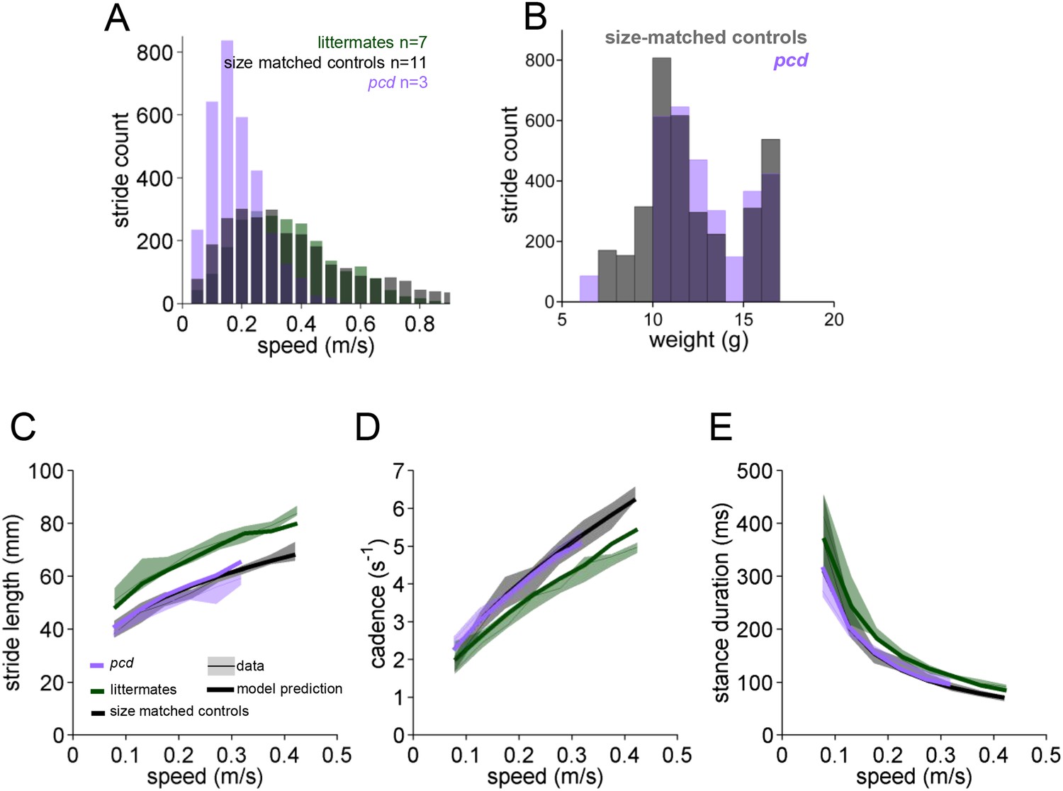
Basic stride parameters for pcd are are not different from their size-matched controls.
(A) Histogram of walking speeds, divided in 0.05 m/s speed bins for pcd (purple, N = 3 mice, n = 3052 strides), littermate controls (green, N = 7 mice, n = 2256 strides) and size matched controls (black, N = 11 mice, n = 3400 strides). (B) Histogram of stride counts by weight for size-matched controls and pcd. (C–E) Basic stride parameters. For each parameter, thick lines represent the prediction, from the mixed-effects models derived from wildtype data in Figure 2 (including speed and weight as predictor variables), for each group. Pcd (average weight = 12g; purple line), control littermates (average weight = 26g; blue line) and size-match controls (average weight = 12g; black line). (C) Stride length values vs walking speed for pcd, littermate controls and size-matched controls (median ±25th, 75th percentile). Data are represented by thin lines and shadows, thick lines are model predictions. (D, E) Temporal measures of the step cycle; cadence (inverse of stride duration) and stance duration, respectively (median ±25th, 75th percentile).
Figure 3—figure supplement 2
3D paw trajectories for wildtype controls and pcd.
(A–C) Average 3D trajectories for front right paw of wildtype control group (N = 34; n = 9602 strides) during swing phase. Traces are binned and color coded by walking speed. (A) Instantaneous forward (x) velocity. (B) side-to-side (y) excursion (C) vertical (z) position relative to ground. (D–F) Same as above but for hind right paw of wildtype control group. (G–I) Paw trajectories for pcd and size-matched controls. (G) Hind right paw x-trajectories. (H) Hind right paw vertical (z) position relative to ground during swing. In pcd, hind paws were lifted higher than forepaws, and their peak positions varied more steeply with speed, (F[153.02,1] = 5.64,p < 0.05).
Figure 4 with 1 supplement
Front-hind limb coordination is specifically impaired in pcd.
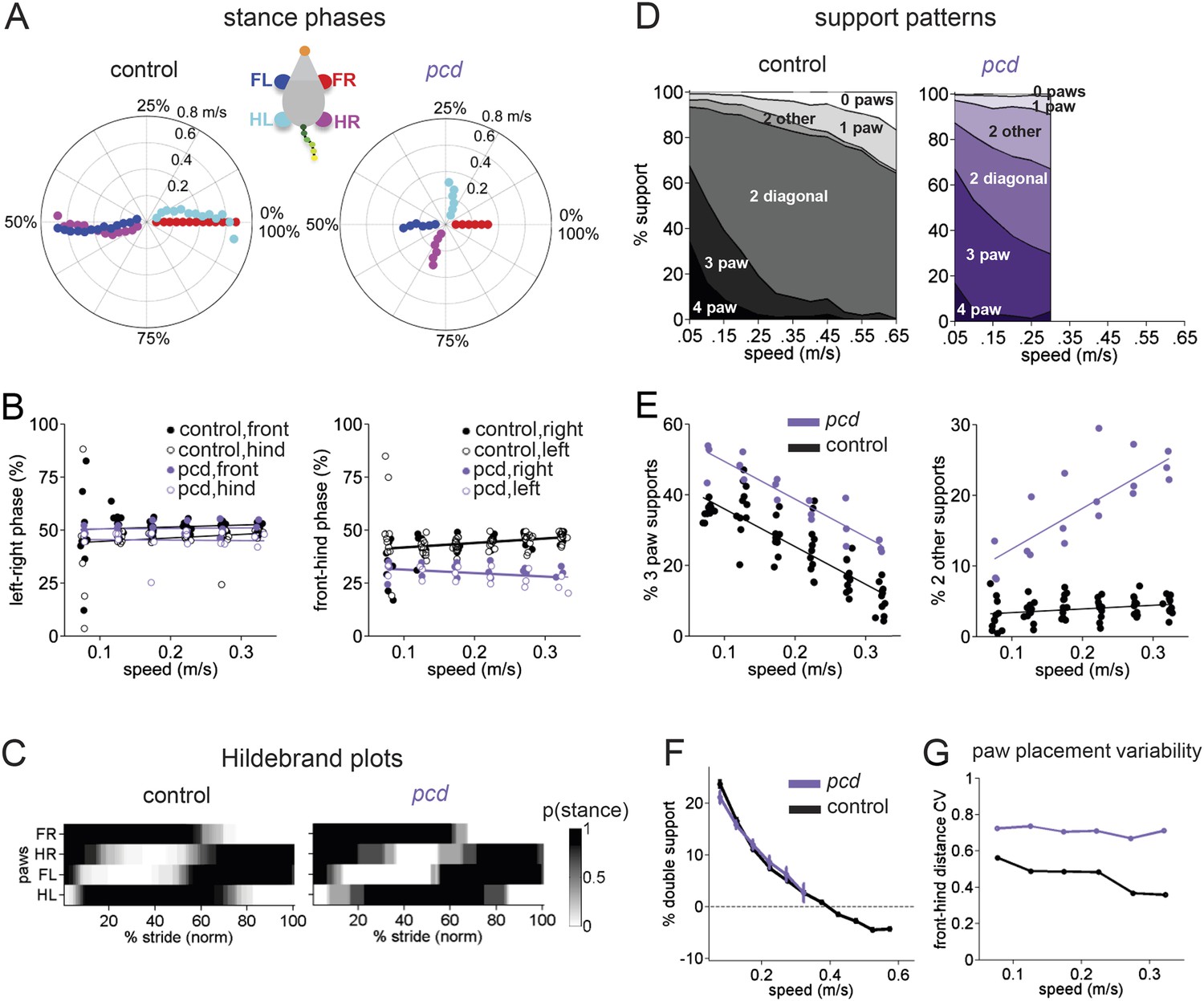
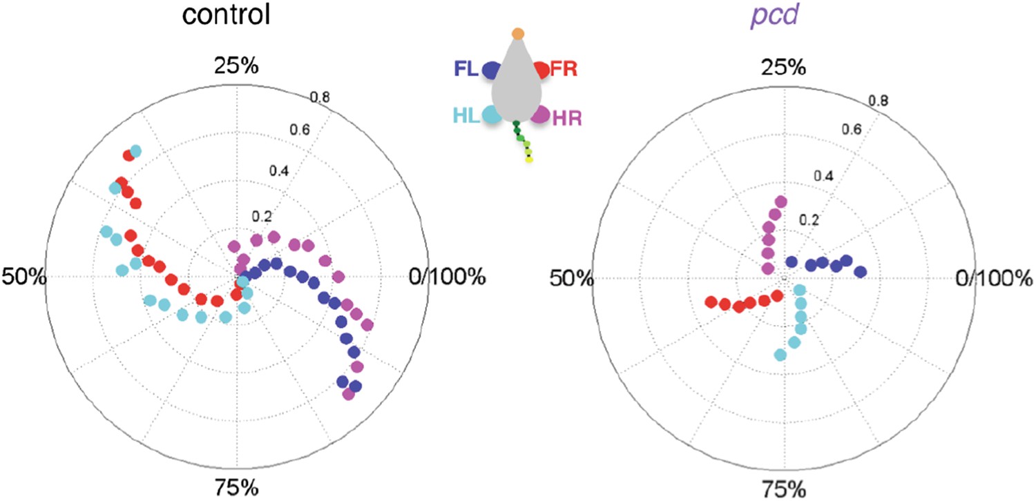
(A) Polar plots indicating the phase of the step cycle in which each limb enters stance, aligned to stance onset of FR paw (red). Distance from the origin represents walking speed. Left, size-matched control mice (N = 11). Right, pcd (N = 3). (B) Left-right phase (left) and front-hind (right) phase for individual animals of pcd and size-matched controls. Circles show average values for each animal. Lines show fit of linear-mixed effects model for each variable. (C) Average Hildebrand plots aligned to FR stance onset for speeds between 0.15 and 0.20 m/s. Grayscale represents probably of stance. (D) Area plot of average paw support types as % of stride cycle, across speeds for size-matched controls (left) and pcd (right). (E) 3 paw (left) and 2-paw other (right) supports for each animal (circles). Lines show fit of linear-mixed effects model. (F) Average ±sem percent double support for hind paws of pcd and size-matched controls. (G) Coefficient of variation for paw placement distance (front-hind) for pcd and size-matched controls.
Figure 4—figure supplement 1
Comparison of gait patterns between control and pcd mice.
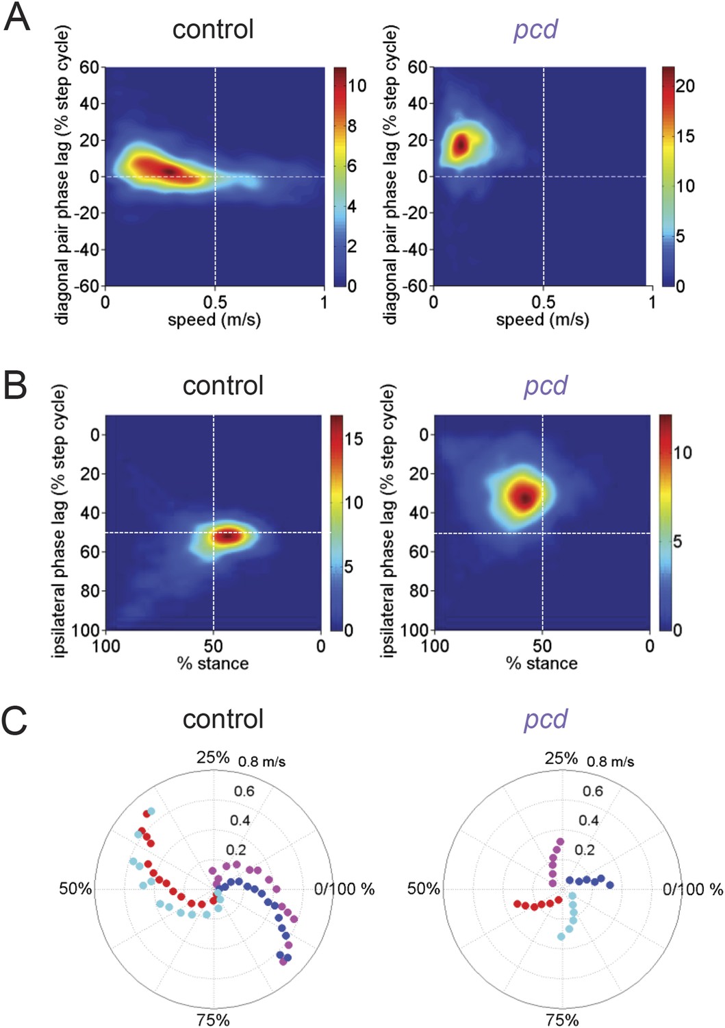
(A) Smoothed probability density of diagonal (FL-HR) pair stance phase lags and speed obtained by kernel density estimation for all strides of size-matched controls (left, n = 3400, N = 11) and pcd (right, n = 3052, N = 3). Color code is estimated stride density. (B) Smoothed probability density of ipsilateral pair (FL-HL) stance phase lags and % stance duration for all strides of size-matched controls (left) and pcd (right), plotted according to the convention of Figure 5 of Hildebrand (1989). Color code is estimated stride density. (C) Polar plots of stance to swing phasing aligned to front right paw for controls (left) and pcd (right).
Figure 5 with 2 supplements
The tail and nose movements of pcd mice can be modeled as a passive consequence of the forward motion of the hind limbs.
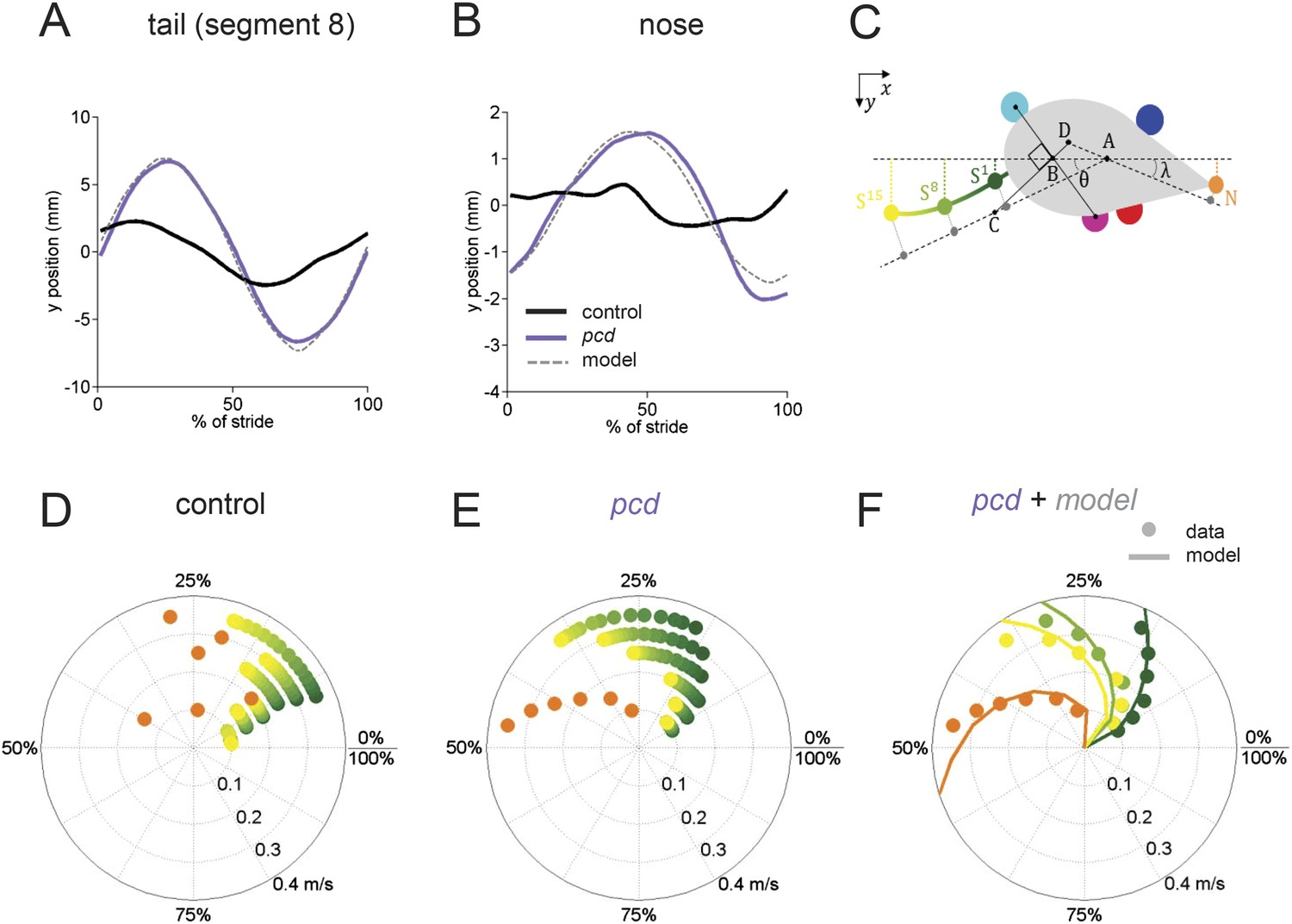
(A, B) Averaged lateral trajectory of tail segment 8 (A) and nose (B), relative to the mid-point between the hind paws, for animals walking at 0.25–0.30 m/s, for size-matched controls (black), pcds (purple) and model (dashed gray). (C) Geometric model of the tail and nose. The lateral position of each tail segment at every time step is given by Syi =_ASisinθ, whereas the lateral position of the nose is given by Ny=_DN _sinλ. (D, E) Phase of maximum correlation between the forward position of the hind paws and the lateral trajectories of each tail segment (green-yellow gradient) and the nose (orange). (F) The maximum correlation phases of the passive geometric model (lines) are superimposed on the observed values (circles) for tail segments 1 (dark green), 8 (light green), 15 (yellow), and nose (orange).
Figure 5—figure supplement 1
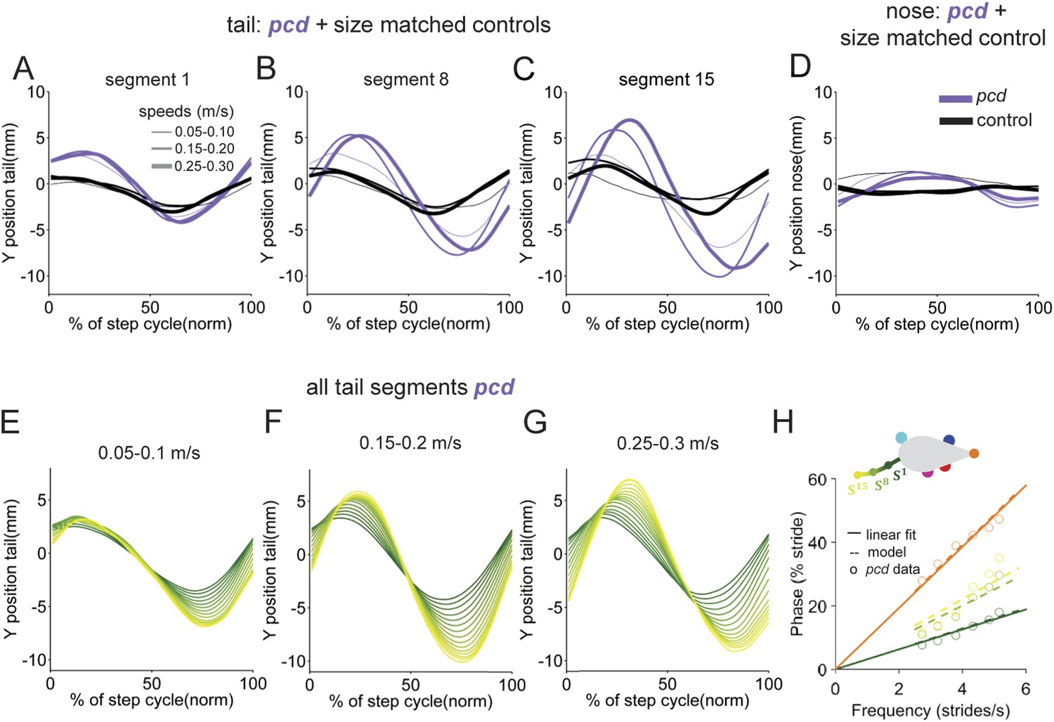
Nose and tail movements across speed bins.
(A–C) Average interpolated (y) trajectory of segment 1, 8, 15, respectively for wild type mice aligned with stance onset of the hind right paw. (D) Average interpolated (y) trajectory of nose for wild type mice aligned with stance onset of the front right paw. (E–G). Average interpolated (y) trajectory of all tail segments for pcd mice aligned to stance onset of the hind right paw across several speed bins. (H) Bode plot of tail and nose phases for pcd.
Figure 5—figure supplement 2
Results summary for young pcd and size-matched controls.
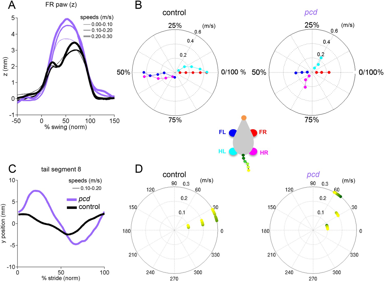
(A) Average vertical (z) position of FR paw relative to ground during swing for young (<P55) pcd (purple) and size-matched controls (compare with Figure 3G). Line thickness represents increasing speed. (B–D) Polar plots indicating the phase of the step cycle in which each limb enters stance, aligned to stance onset of FR paw (red). Distance from the origin represents walking speed. Left, size-matched control mice. Right, young pcd (compare with Figure 4A). (C) Averaged lateral trajectory of tail segment 8 relative to the mid-point between the hind paws, for animals walking at 0.1–0.2 m/s, for size-matched controls (black), and young pcd (purple) (compare with Figure 5A). (D) Phase of maximum correlation between the forward position of the hind paws and the lateral trajectories of each tail segment (green-yellow gradient) for size-matched controls (left) and pcd (right) (compare with Figure 5D,E).
Figure 6

Visualization of impaired whole-body coordination in pcd.
(A) Ribbon plots showing average vertical (z) trajectories for nose, paw and select tail (2, 5, 8, 11, 14) segments for size-matched control (Left, N = 11)) and pcd (Right, N = 3) mice walking at 0.20–0.25 m/s. Data are presented relative to 100% of the stride cycle of the FR paw (x-axis). Nose and paw trajectories are z position relative to floor; tail is z relative to floor with mean vertical position of the of base of the tail subtracted for clarity. (B) Matrix of correlation coefficients computed for average vertical trajectories of control (Left) and pcd (Right). Color bar is value of correlation coefficient.
Author response image 1
Stance to swing phases for size-matched controls and all pcd.
https://doi.org/10.7554/eLife.07892.023
Author response image 2

Average Hildebrand plots aligned to FR stance onset.
https://doi.org/10.7554/eLife.07892.024
Author response image 3
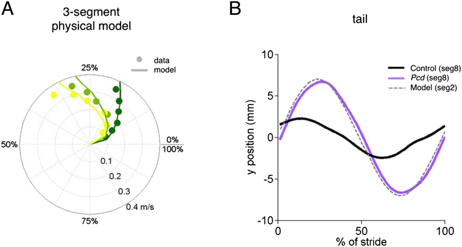
Physical model.
The physical model of the tail consists of three masses 1, 2 and 3 (the later being the most distal) connected via an angualar spring-damper system. The masses of each segment were estimated from measurements of a real mouse tail (10g, 0.6g, 0.001g for segments 1, 2 and 3 respectively). The springs and dampers were estimated manually (k1=13e-6 Nm/deg, c1=0.95e-6 Nms/deg, k2=5e-6 Nm/deg, c2=0.7e-6 Nms/deg and k3=20e-6 Nm/deg, c3=0.2e-6 Nms/deg). The model was implemented and tested in SimMechanics MATLAB 2015a. (A) The phases of segments 1, 2 and 3 in the model (lines) superimposed over segments of 18 and 15 of the pcd tail. (B) Trajectories of tail segment 8 for controls (black), and pcd (purple), and tail segment 2 for the physical model.
Videos
Video 1
Automated, high-resolution locomotion tracking in freely walking mice.
High-speed (400 fps) video of a mouse crossing the LocoMouse corridor, displayed at 30 fps. Side and bottom (via mirror reflection) views of the mouse are captured in a single camera. Top: Raw video of a wild-type mouse. Bottom: Same video with the output of the machine learning tracking overlaid: nose (orange circle), paws (red: front right; blue: front left; magenta: hind right; cyan: hind left) and tail segments (green-to-yellow gradient circles).
Video 2
Purkinje cell degeneration mice are visibly ataxic.
Purkinje cell degeneration (pcd) mouse crossing the LocoMouse corridor. Pcd mice are smaller and walk more slowly than controls. They lift their paws higher and have altered patterns of interlimb coordination. The nose and tail oscillate laterally and vertically.
Video 3
Passive nose and tail model.
Passive model of nose and tail for a mouse walking at 0.2 m/s. The forward movements of the paws were modeled according to the data described in Figures 3 and 4. The lateral movements of the nose and tail segments are predicted from a model in which an orthogonal projection transforms the forward movements of the hind paws (solid white line) into lateral movements of the tail (dashed white line) and nose with a fixed time-delay for each element. As a result of this orthogonal coupling, the nose and tail oscillate laterally as a passive consequence of the forward motion of the hind paws.
Tables
Table 1
Image feature size
| Feature | Bottom view size (in pixels) | Side view size (in pixels) |
|---|---|---|
| Paw | 30 x 30 | 20 x 30 |
| Snout | 40 x 40 | 20 x 40 |
| Tail segments | 30 x 30 | 25 x 30 |
Download links
A two-part list of links to download the article, or parts of the article, in various formats.
Downloads (link to download the article as PDF)
Open citations (links to open the citations from this article in various online reference manager services)
Cite this article (links to download the citations from this article in formats compatible with various reference manager tools)
A quantitative framework for whole-body coordination reveals specific deficits in freely walking ataxic mice
eLife 4:e07892.
https://doi.org/10.7554/eLife.07892


