Sensory dynamics of visual hallucinations in the normal population
- University of New South Wales, Australia
- University of Pittsburgh, United States
Figures
Figure 1
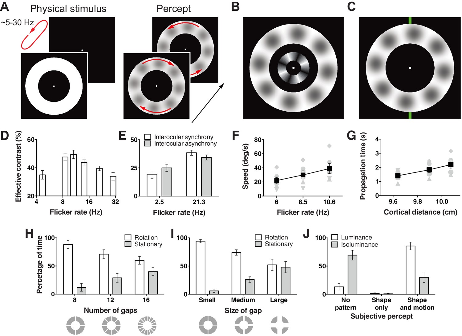
Hallucination stimulus and data.
(A) Physical stimulus and depiction of the percept. (B) Depiction of the stimulus used to measure the effective contrast. The small inner annulus is the perceptual, while the larger outer annulus shows a depiction of the hallucinated content. (C) Hallucination depiction and nonius lines used to measure the effective rotation propagation times. (D) Effective contrast data showing mean point of subjective equivalence between the perceptual and hallucinated content as a function of flicker frequency (Exp. 1; N = 42, 56 trials per frequency). (E) Data showing interocular interaction (Exp. 2; N = 20, 56 trials per combination of synchrony and frequency). Synchronous and asynchronous flickering annuli give different contrasts measures. (F) Hallucination motion speed measures using stimulus in C, as a function of flicker rate (Exp. 3A; N = 6, 40 trials per frequency). (G) Dependence of propagation times on cortical distance (Exp. 3B; N = 6, 40 trials per eccentricity condition). Distance around the annulus was converted into cm across cortex using the formulae from (Horton and Hoyt, 1991). Main effect of distance F(2, 5) = 13.74; p=0.001. (H) The effect of number of physical gaps in the annulus (Exp. 4A; N = 4, 10 trials per stimulus). (I) The effect of the width of physical gaps in the annulus (Exp. 4B; N = 4, 10 trials per stimulus). (J) Hallucinated structure and motion is reduced at isoluminance (Exp. 5; N = 5, 20 trials per luminance condition). All error bars show ± SEM.
Figure 2
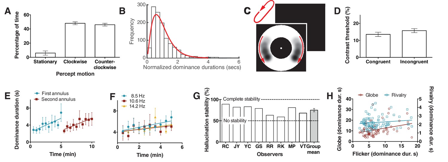
Bistability of the hallucination.
(A) Data showing that subjects experience the hallucination rotation equally in clockwise and counter-clockwise directions (Exp. 6; N = 9, 10 min of tracking). (B) A histogram of dominance durations, showing the long tail and fit with a gamma function, a hallmark of perceptual bistability (Exp. 6; from the gamma fit: a = 2.49; b = 0.40). (C) Depiction of the motion probe stimulus. Motion probes were presented moving clockwise or counter-clockwise, while subjects tracked hallucination alternations. (D) Contrast thresholds from the probe stimulus for congruent and incongruent probes (Exp. 7; N = 13, 384 trials). (E) Longer dominance durations over viewing time suggest a form of adaptation that is local in visual space, the second ring ‘resets’ the adaptation (Exp. 8A; N = 7, 10 min tracking per stimulus order). (F) Dominance durations over time for three different flicker frequencies (Exp. 8B; N = 6, 10 trials per frequency). (G) 8 individual subjects and the mean stability for intermittent physical presentations (Exp. 9; 100 trials). (H) Comparing dominance durations in binocular rivalry, rotation globe-stimulus and flicker hallucinations (Exp. 10; N = 84, 2 trials of two minutes tracking). Retest reliability: flicker: r =0.736; globe: r =0.741; rivalry: r =0.744; all ps <0.0001. All error bars show ± SEM.
Figure 3 with 1 supplement
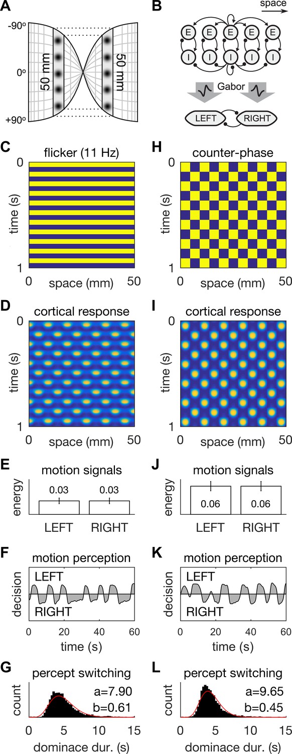
A neural field model of flicker-induced bistable motion.
(A) The log-polar retinotopic map of human visual cortex. The fovea is located at the centre. The annulus stimulus maps onto a thin strip of tissue (shaded) that spans both hemispheres. Inter-hemispheric fibres (dotted lines) connect the strips to form a contiguous ring. (B) Schematic of the model. The ring of tissue is modelled in one spatial dimension using an established neural field model (Rule et al., 2011). that comprises local populations of excitatory (E) and inhibitory (I) cells. Flicker and counter-phase stimulation both induce counter-phase responses in this model. Motion within the cortical response patterns was detected by banks of Gabor filters (large arrows) following the motion-energy model. The motion-energy signals (boxes) represented the percepts of LEFT (anti-clockwise) and RIGHT (clockwise) motion. Those percepts were subject to rivalry through mutual inhibition and firing rate adaptation. (C) Space-time plots of flicker. (D) Cortical responses to flicker. (E) Time-averaged LEFT and RIGHT motion-energy responses to flicker stimulation. Error bars are ±1 standard deviation. (F) Time course of the perceptual decisions evoked by flicker. (G) Histogram of dominance durations for switching between left and right motion percepts fit with a gamma function. The variation in switch times is due to injected noise in perceptual rivalry model. (H–L) The analogous representations for the counter-phase retina-sourced stimulation.
Figure 3—figure supplement 1
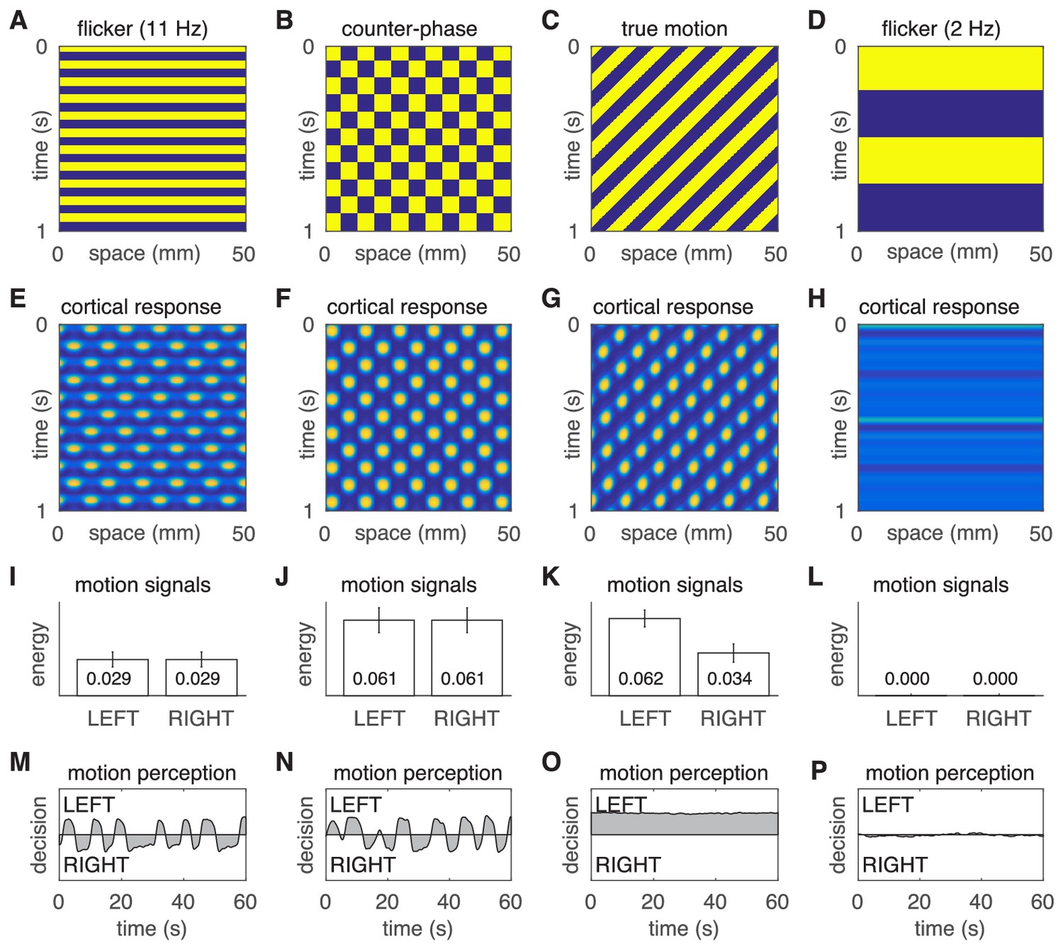
Motion percepts in the model under four different stimulus conditions.
(A–D) Space-time plots of the four stimuli. (E–H) Space-time plots of the corresponding cortical responses. (I–L) Time- averaged responses of the LEFT and RIGHT motion detectors. (M–P) Time courses of the perceptual decisions. The two left most columns reproduce the results of the main text, namely the comparison of illusory motion induced by flicker and counter-phase stimulation. The two rightmost columns demonstrate the absence of illusory motion in response to true motion and slow strobe-like flicker stimulation.
Author response image 1
Videos
Video 1
An animated movie representation of one of our stimuli.
Under the right viewing conditions, you may experience light grey blobs (that are not physically presented in the movie) appearing around the flickering annulus. This video contains flashing and alternating images, and therefore might not be suitable for readers with photosensitive epilepsy.
Video 2
A perceptual, retina-based representation approximating what some see in the otherwise empty flickering white annulus of Video 1.
Note, this is only one interpretation, the individual hallucination experience may vary from individual to individual. This video contains flashing and alternating images, and therefore might not be suitable for readers with photosensitive epilepsy.
Tables
Appendix 1—table 1
Parameters of the cortical model.
| Parameter | Description |
|---|---|
| Excitatory activation state | |
| Inhibitory activation state | |
| Spatio-temporal stimulus | |
| Spatial coupling kernel | |
| Spread of excitation (mm) | |
| Spread of inhibition (mm) | |
| Coupling weight ( to ) | |
| Coupling weight ( to ) | |
| Coupling weight ( to ) | |
| Coupling weight ( to ) | |
| Excitatory firing threshold | |
| Inhibitory firing threshold | |
| Excitatory time constant (ms) | |
| Inhibitory time constant (ms) | |
| Ring length (mm) | |
| Spatial resolution (mm) | |
| Integration time step (ms) | |
| Spatial frequency (cycles/mm) | |
| Temporal frequency (cycles/ms) |
Download links
A two-part list of links to download the article, or parts of the article, in various formats.
Downloads (link to download the article as PDF)
Open citations (links to open the citations from this article in various online reference manager services)
Cite this article (links to download the citations from this article in formats compatible with various reference manager tools)
Sensory dynamics of visual hallucinations in the normal population
eLife 5:e17072.
https://doi.org/10.7554/eLife.17072


