Generation of shape complexity through tissue conflict resolution
- John Innes Centre, England
- University of East Anglia, England
Figures
Figure 1 with 1 supplement
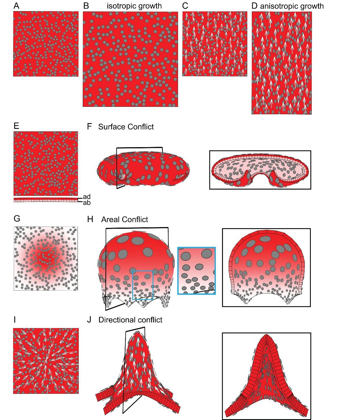
Generation of 3D deformations through tissue conflict resolution.
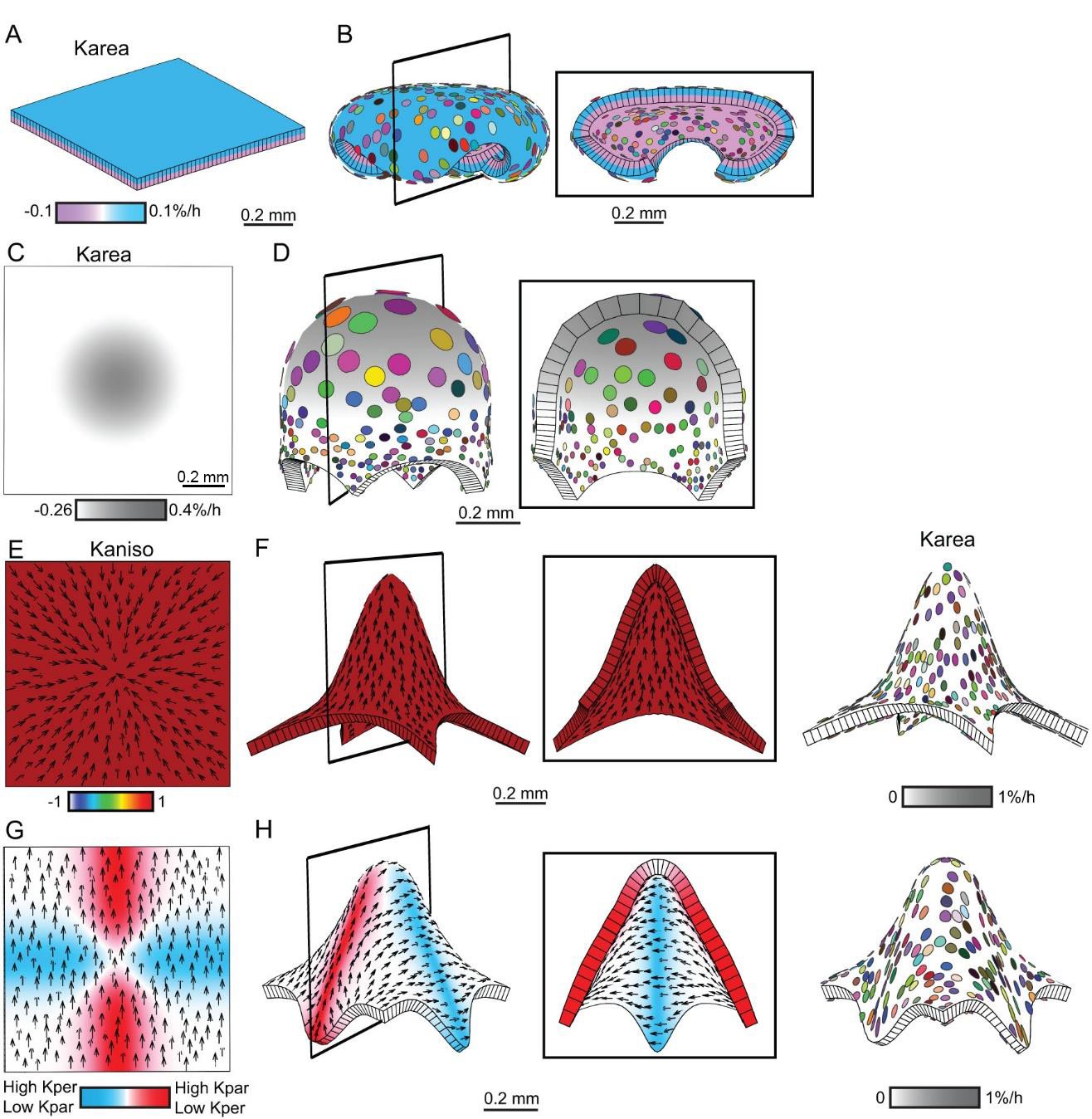
(A–B) Isotropic specified growth promoted by a uniformly expressed Growth-promoting Transcription Factor (GTF, red shading). The initial square marked with circular clones (A) grows into a bigger square with enlarged isometric clones (B). (C–D) A proximodistal polarity field (white arrows) with uniformly expressed GTF promoting growth parallel to the polarity (specified anisotropic growth). The square (C) elongates to from a rectangle (D). (E–F) Surface conflict. GTF promotes specified isotropic growth and is expressed at a higher level in the top surface (red, adaxial, ad) compared to the bottom (pink, abaxial, ab) (E). The canvas deforms into a dome with downwards curled edges (F). (G–H) Areal conflict. GTF promotes specified isotropic growth and is more highly expressed in the centre of the canvas (G). The canvas deforms into a rounded dome with circular clones bigger at the apex (H, side view in left panel and clipped view in right panel) and slightly elliptical at the periphery of the dome (blue square in H). (I–J) Directional conflict with a convergent polarity field (white arrows) and GTF promoting growth parallel to the polarity. The square deforms into an elongated dome with clones elongated parallel to the polarity field (J, side view in left panel, clipped view in right panel). For each model the position of the clipping plane is indicated by black line in the side view.
Figure 1—figure supplement 1
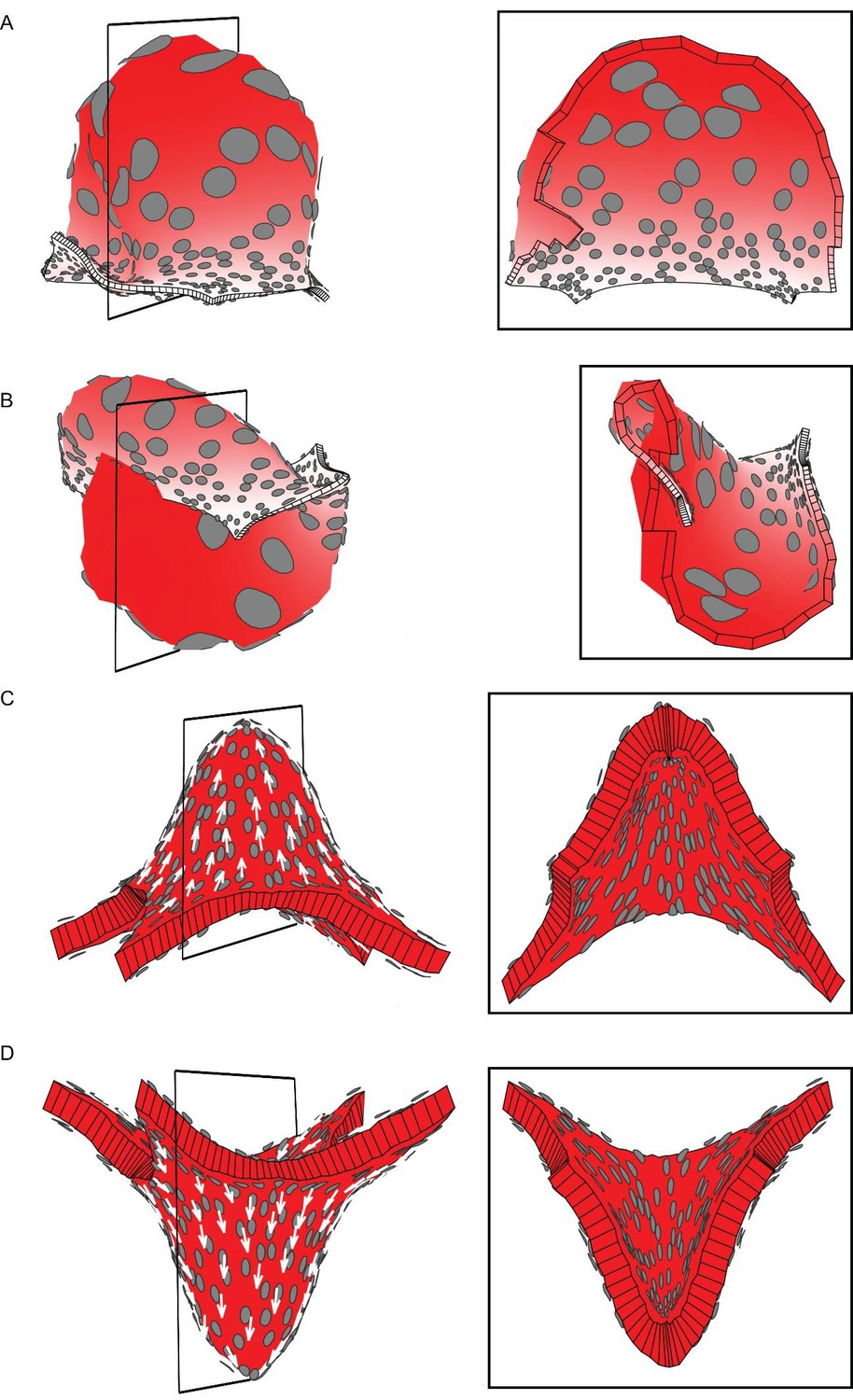
Areal and directional conflicts with flat starting tissue.
Tissue conflict resolutions as in Figure 1 but starting with a flat sheet with a small amount of random perturbation in height instead of an initial slight curvature. (A–B) Areal conflict as in Figure 1G. The tissue buckles to form a dome or wave depending on the simulation run (A and B are outputs from two separate runs). (C–D) Directional conflict as in Figure 1I. The tissue buckles to form a dome upwards or downwards depending on the simulation run (C and D are outputs from two separate runs).
Figure 2
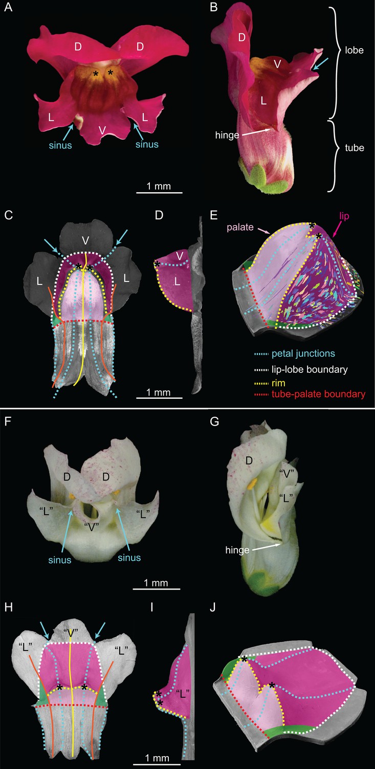
Wild-type and div Snapdragon corolla morphology.
(A–E) Wild-type bilaterally symmetric Snapdragon flower, with dorsal (D), lateral (L) and ventral (V) petals (A). The flower has a closed mouth hinged at the dorsal to lateral sinuses (hinge). The corolla is divided into a proximal region (tube) and distal region (lobes) (B). Dissected and partially flattened lower petals, imaged from above (C, adaxial surface, i.e. inside the flower) and side (D) (black and white images are used to allow labelling of petal regions). Along the proximodistal axis, the distal wedge limit is the boundary between the lip and the distal lobe (white dashed line), and the proximal wedge limit is the boundary between the palate and the proximal tube (red dashed line). Along the mediolateral axis, the lateral petal midveins (orange lines) are the lateral wedge limits. Ventral petal midvein (yellow line), petal junctions (blue dashed lines), foci (asterisks) and petal sinuses (blue arrows) are also labelled. A simplified clay model of the wedge shape (E) illustrates the slope (palate, light pink), ridge (rim, yellow dashed line) and cliff (lip, dark pink). Experimentally induced clonal sectors (Green et al., 2010) are superimposed on the 3D shape (multi-coloured regions). The wedge spans the ventral petal and the ventral half of the lateral petal (flanks) while the dorsal half of the lateral petal forms a narrow region either side (hinge, green shading in C and E). (F–J) div mutant flower, with normal dorsal petals (D), modified lateral and ventral petals (‘L’ and ‘V’) (F), and an open flower (G). To compare the shape of the div mutant with wild type, the div mutant lower petals were dissected, flattened, imaged from above (H, adaxial side) and from the side (I) and labelled as for wild type. The div mutant has two domes at the foci (asterisks in H–J). A simplified clay model (J) highlights the reduction of palate (light pink shading) and the flat lip (dark pink shading).
Figure 3
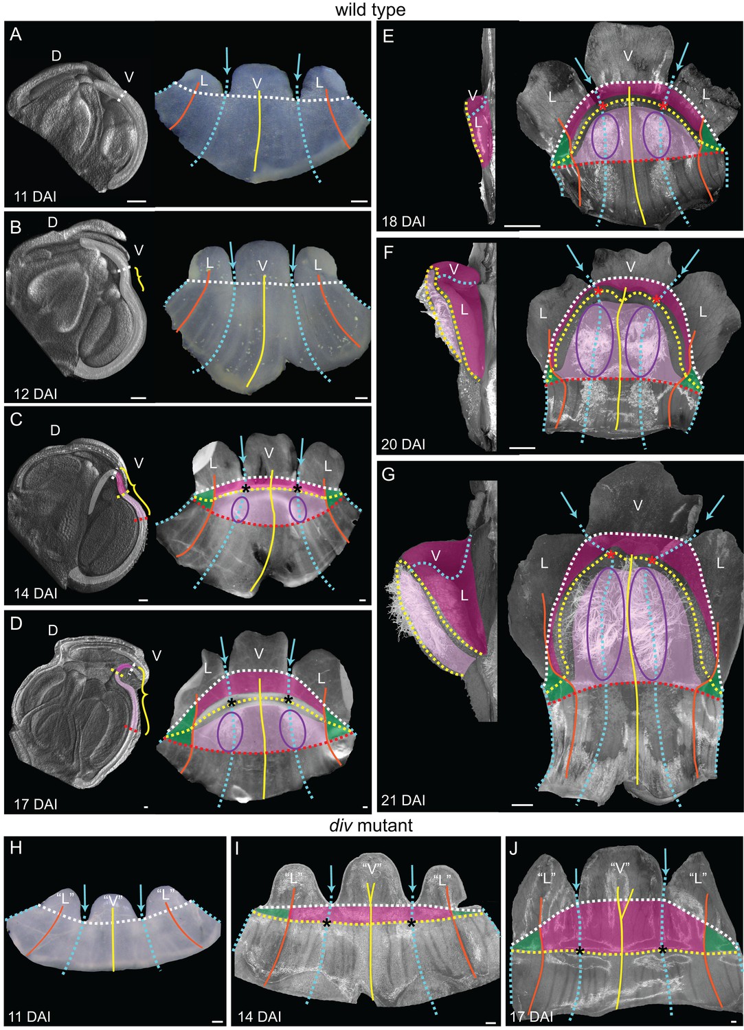
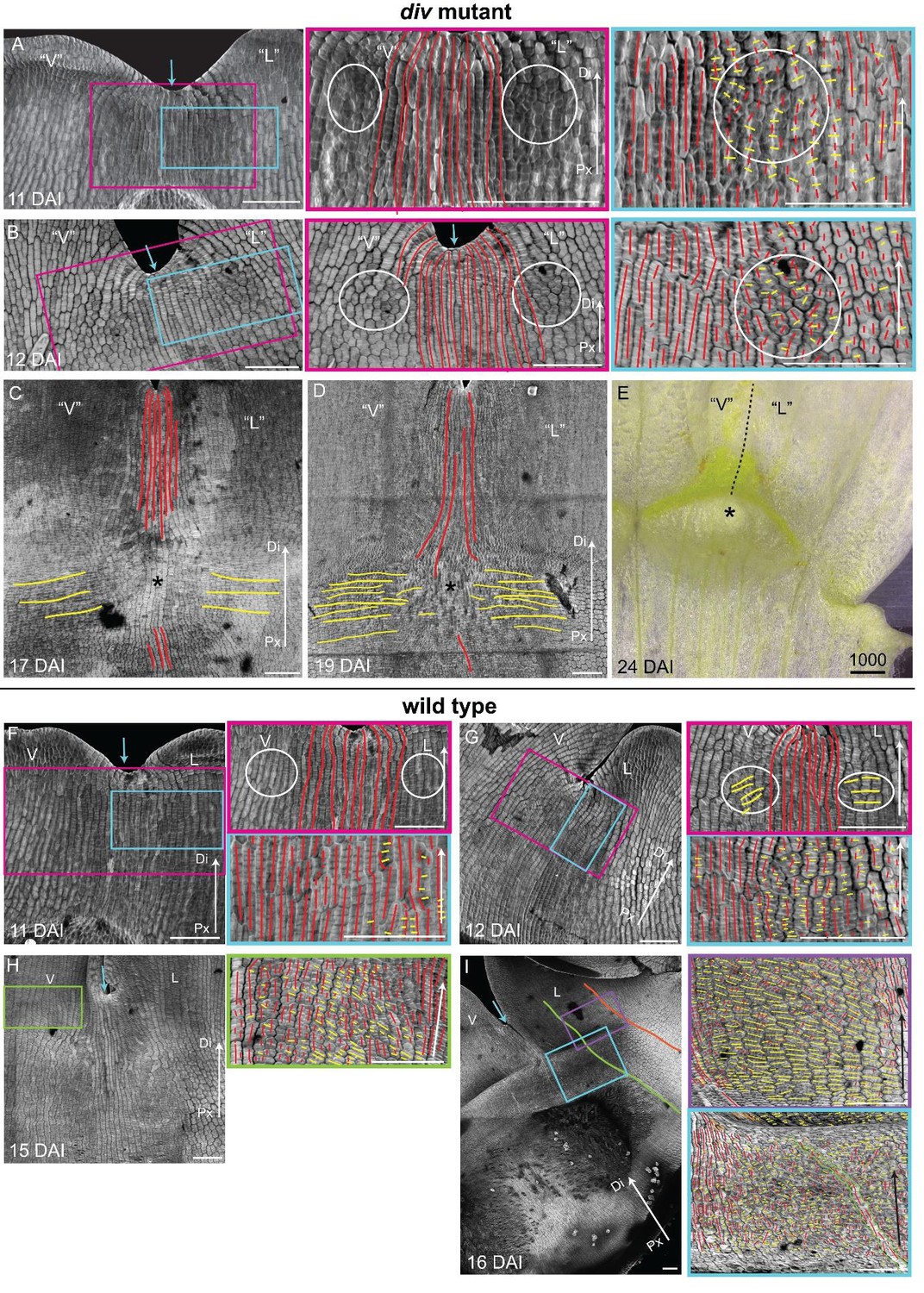
Morphogenesis and fate map of div and wild-type lower corollas.
(A–G) Fate map of wedge emergence in the wild-type lower corolla. The 3D deformation of the lower petals was visualised by OPT (Lee et al., 2006) with a longitudinal midsection across the ventral petal (highlighted with white shading in left panels of A-D) and by photographing the partially flattened lower corolla (right panels), labelled with various morphological landmarks as Figure 2. The boundary between the palate and the proximal tube (red dashed line) can only be determined after palate trichome emergence at 14 DAI (purple ellipses). At early stages of development, 11 DAI (A) and 12 DAI (B), the lower petals develop a furrow at the rim (yellow bracket in B) although they still appear relatively flat. During the next five days (C and D), the furrow gets more pronounced and can be clearly seen at 17 DAI (yellow bracket in D). From 18 DAI, the out-of-plane deformation is visible from side (left panel in E-G) and top (right panel in E-G) views of the dissected corolla. The size of the wedge increases over the next four days (compare E to G). Scale bars, 100 µm (A–D) and 1 mm (E–G). (H–J) Fate map of dome emergence in the div lower corolla. The div lower corolla was dissected and partially flattened at 11 DAI (H), 14 DAI (I) and 17 DAI (J), and labelled with various morphological landmarks as for wild type, except for the boundary between the palate and the proximal tube, which is difficult to determine at these stages due to the lack of palate trichomes. Initially, petals are relatively flat (H). At 14 DAI small adaxial bulges, with foci at their tips (asterisks in I), can be seen at the intersection between the petal junctions and the rim. This is also the first timepoint when the lip region can be mapped (dark pink). By 17 DAI, the domes extend half way into the lateral petals (orange line in J). Scale bars, 100 µm.
Figure 4 with 1 supplement
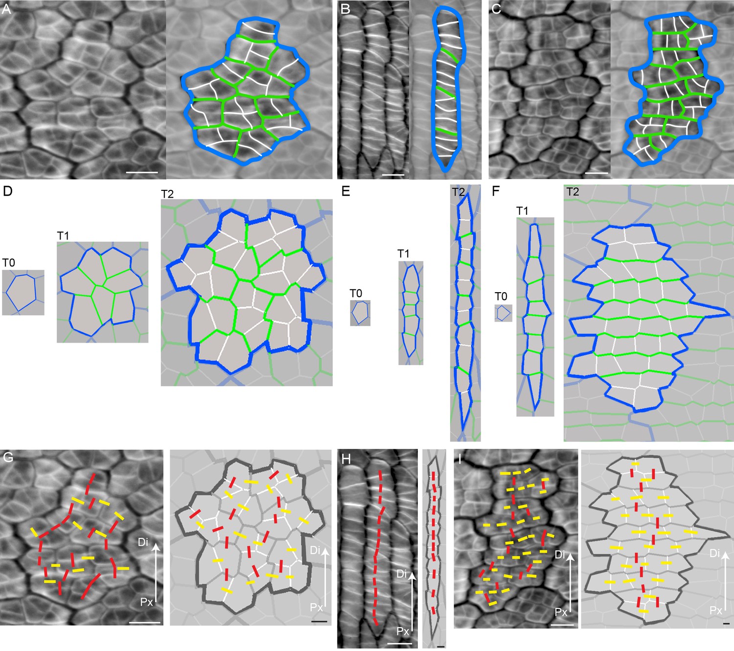
Inferring growth orientations from cell division patterns.
(A–C) Confocal images of petal tissue showing different shapes of cell files (or clones). The cell walls were stained with calcofluor white (left panels). The most recent cell walls stain the brightest and are the thinnest (indicated by the white lines), intermediate cell walls stain less and are thicker (green lines), and the oldest cell walls are the thickest and hardly stain (blue lines). The three examples show different patterns observed on developing petals. Scale bars, 10 μm. (D–F) Simulated growth patterns that generate the shape of cell files (or clones) and pattern of cell divisions depicted in A–C. Original cell wall (T0) blue, cell walls formed during T1 in green (thinner than the T0 cell walls), and cell walls formed at T2 in white (the thinnest cell walls). Specified growth isotropic (D), oriented vertically (E), or oriented vertically and then switching to horizontal (F). Scale bars, 10 μm. (G–I) Inferring growth orientations from the patterns of cell division in the calcofluor data using lines perpendicular to cell division walls. For each panel, biological data is shown on left, simulation output on right. Lines were classified as roughly parallel (red) or perpendicular (yellow) to the proximodistal axis (Px-Di for data) or to the orientation of specified growth (simulations). The simulations show output for isotropic growth (G) vertically oriented specified growth (H) or vertical followed by horizontally oriented specified growth (I). Scale bars, 10 μm.
Figure 4—figure supplement 1
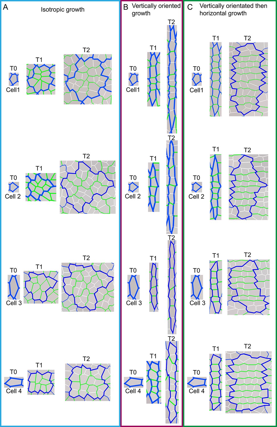
Model output of cell division patterns generated from different specified growth patterns with various initial cell geometries.
(A-C) Model output of cell files (or clones) and pattern of cell divisions for four different starting cell shapes under three different growth conditions. For each starting cell shape (T0), two images are captured at subsequent times, T1 and T2, under specified isotropic growth (A), vertically oriented growth (B) and vertically orientated and then switching to horizontal growth (C). Original cell walls are shown in blue (T0), initially new cell walls are drawn in green (T1) and then at later times drawn in white (T2). Note that in (A) new walls (green and white) are randomly orientated; in (B) new walls are mainly horizontal and in (C) green walls are mainly horizontal and white walls are mainly vertical. Thus initial cell wall geometry does not have a major effect on cell wall patterns.
Figure 5 with 2 supplements
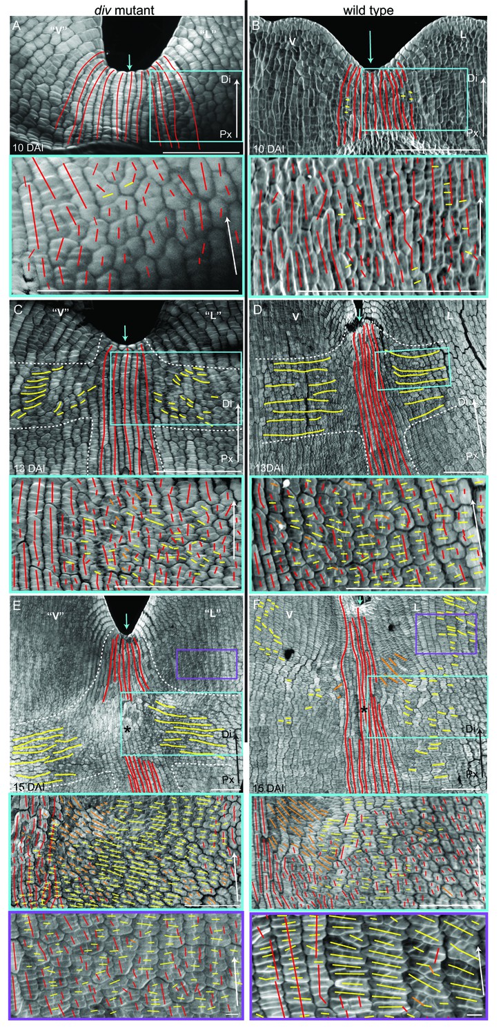
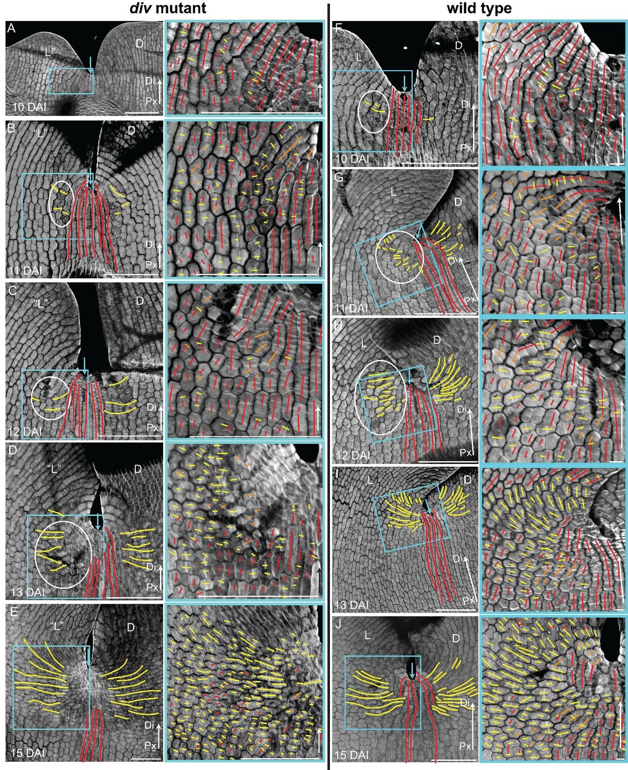
Pattern of cell file orientations at the ventral-lateral junctions during div and wild-type development.
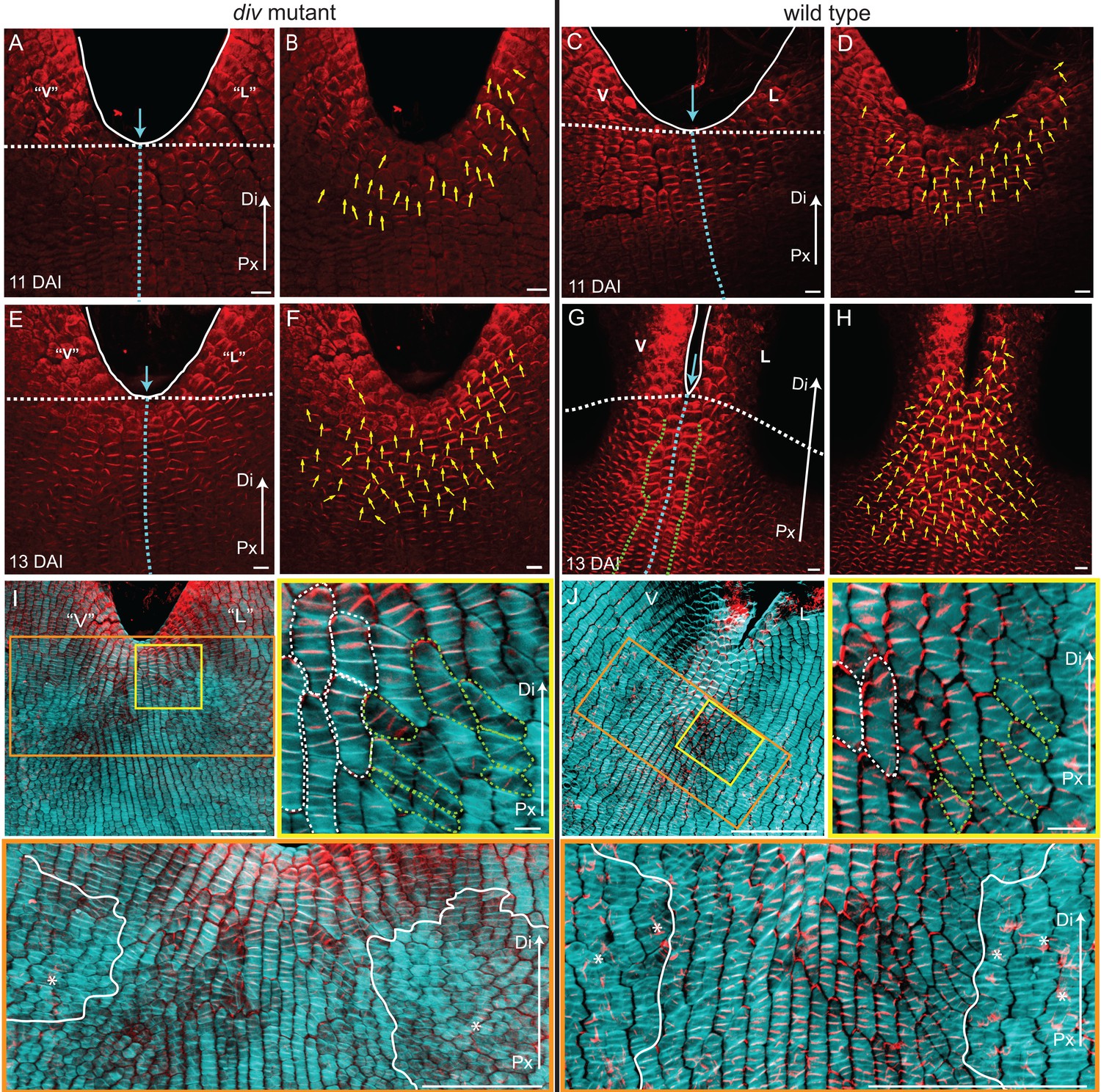
(A–F) Confocal images of div and wild-type ventral-lateral (V–L) junctions at 10 DAI (A and B), 13 DAI (C and D) and 15 DAI (E and F). The tissue was stained with calcofluor white to visualise the patterns of cell division and infer growth orientations as described in Figure 4G–H: proximodistal growth (red lines), mediolateral growth (yellow lines) and diagonal growth (orange lines). Each stage is shown in two magnifications: an overview of the junction region and a zoomed-in region (coloured boxes in A-F). Only regions showing the clearest cell files and oriented patterns of division are shown in the overview images. The patterns of cell files at the div and wild-type V-L junction are mainly proximodistal at 10 DAI (A and B) and become increasingly mediolateral in the rim regions flanking the junction forming an orthogonal pattern of cell files by 13 DAI (white dashed lines in C and D). At 15 DAI, the mediolateral region expands and together with the proximodistal files at the junction form a clear orthogonal pattern of growth orientations in div (white dashed lines in E). In wild type, the orthogonal pattern is not as clear as the rim region flanking the foci and shows a mix of mediolateral and proximodistal growth (blue box in F) but extends to the lateral lip, where predominantly mediolateral growth is observed (purple box in F) in contrast to the mixed proximodistal and mediolateral growth in the div lateral lip (purple box in E). Arrow at the lower right corner of each. panel indicates Proximal (Px) and Distal (Di) axis. Scale bar 100 μm, except for purple boxes of E and F where scale bar is 10 μm.
Figure 5—figure supplement 1
Pattern of cell file orientations at the ventral-lateral junctions during div and wild-type development.
(A-D) Confocal images of div lower petals, stained with calcofluor white to visualise the pattern of cell files, at different stages of development: 11 DAI (A), 12 DAI (B), 17 DAI (C) and 19 DAI (D). For the early stages (A and B), various maginfications are shown: 1) ‘ventral’ (‘V’) and ‘lateral’ (‘L’) petals (left panel); 2) enlargement (pink box in left panel) of the junction region labelled with the proximodistal files (red lines) and mediolateral files (yellow lines) (middle panels), and 3) enlargement (blue box in left panel) of the ‘lateral’ rim labelled for proximodistal and mediolateral growth (orthogonal to new walls, right panel). Cell files are predominantly proximodistal at early stages in development (more red lines than yellow lines in A and B). The orthogonal pattern of cell files observed at day 15 (Figure 4C) is maintained later in development, at the time the emergence of the div domes (C and D). Proximal (Px) and Distal (Di) axis indicated by arrow at the lower right corner of each panel. Scale bar, 100 μm. (E) Detail of a div ‘ventral-lateral’ junction at maturity (day24). Black dashed line indicatse the LIP boundary between the ‘ventral’ and ‘lateral’ petals. (F-I) Confocal images of wild-type lower petals stained with calcofluor white, at different stages of development: 11 DAI (F), 12 DAI (G), 15 DAI (H) and 16 DAI (I). At each stage, magnifications are shown: 1) ventral (V) and lateral (L) petals (left panel); 2) enlargement of the junction region (pink box in left panel) labelled with the proximodistal files (red lines), mediolateral files (yellow lines) and diagonal lines (orange lines) (top right panel); 3) enlargement of the lateral rim (blue box in left panel) labelled for proximodistal and mediolateral growth (orthogonal to new walls) (bottom right panel); 4) enlargement of the lateral lip, labelled as previous panel (lilac box in left panel of I); 5) enlargement of the ventral lip, labelled as above (green box in left panel of H). Between 10 and 12 DAI (F and G), there is an increase in mediolateral cell files in the rim region flanking (yellow lines within white ellipses) the junctions while in other regions growth is maintained mainly proximodistal (red lines). By 15 DAI, the orthogonal pattern of cell files is not as clear as in div (see Figure 4F). The mediolateral growth regions extend to the lateral (purple box in Figure 4F) and ventral lip (green box, H). This pattern is maintained at later stages when the deformation of the rim region forming the ridge can be observed (I). The positions of the lateral midvein and secondary vein are marked with an orange and green ‘line, respectively, in D. Scale bar, 100 μm.
Figure 5—figure supplement 2
Pattern of cell file orientations at the lateral-dorsal junctions during div and wild-type development.
(A-E) Confocal images of div lower petals, stained with calcofluor white to visualise the cell division orientations, at different stages of development: 10 DAI (A), 11 DAI (B), 12 DAI (C), 13 DAI (D) and 15 DAI (E). At each stage, two magnifications are shown: 1) left panel, an image of the ‘lateral’ (‘L’) and dorsal (D) petal junction labelled for proximodistal cell files (red lines) and mediolateral cell files (yellow lines); 2) right panel, enlarged region (blue box in respective left panel) of the ‘lateral’ rim labelled for proximodistal (red lines) and mediolateral (yellow lines) growth (orthogonal to new walls). Similar to the ‘ventral-lateral’ junction, cell files are mainly proximodistal at early stages in development (A) and become increasingly mediolateral (white ellipses in B, C and D) in the rim region as the petals reach 15 DAI, when a clear orthogonal pattern of cell files can be observed (E). Unlike the ‘ventral-lateral’, the mediolateral files are organised around the sinus (blue arrow), most likely due to the lack of growth at the lip region. Proximal (Px) and Distal (Di) axis indicated by arrow at the lower right corner of each panel. Scale. bar, 100 μm. (F-J) Confocal images of wild-type lower petals, stained with calcofluor, at different stages of development: day 10 (F), day 11 (G), day 12 (H), day 13 I) and day 15 (J). At each stage, two magnifications are shown. The pattern of cell files is similar to the div ‘lateral’-dorsal junction, forming an orthogonal pattern of cell files around the junction. Scale bar, 100 μm and 10 μm (for in zoomed-in images).
Figure 6 with 1 supplement
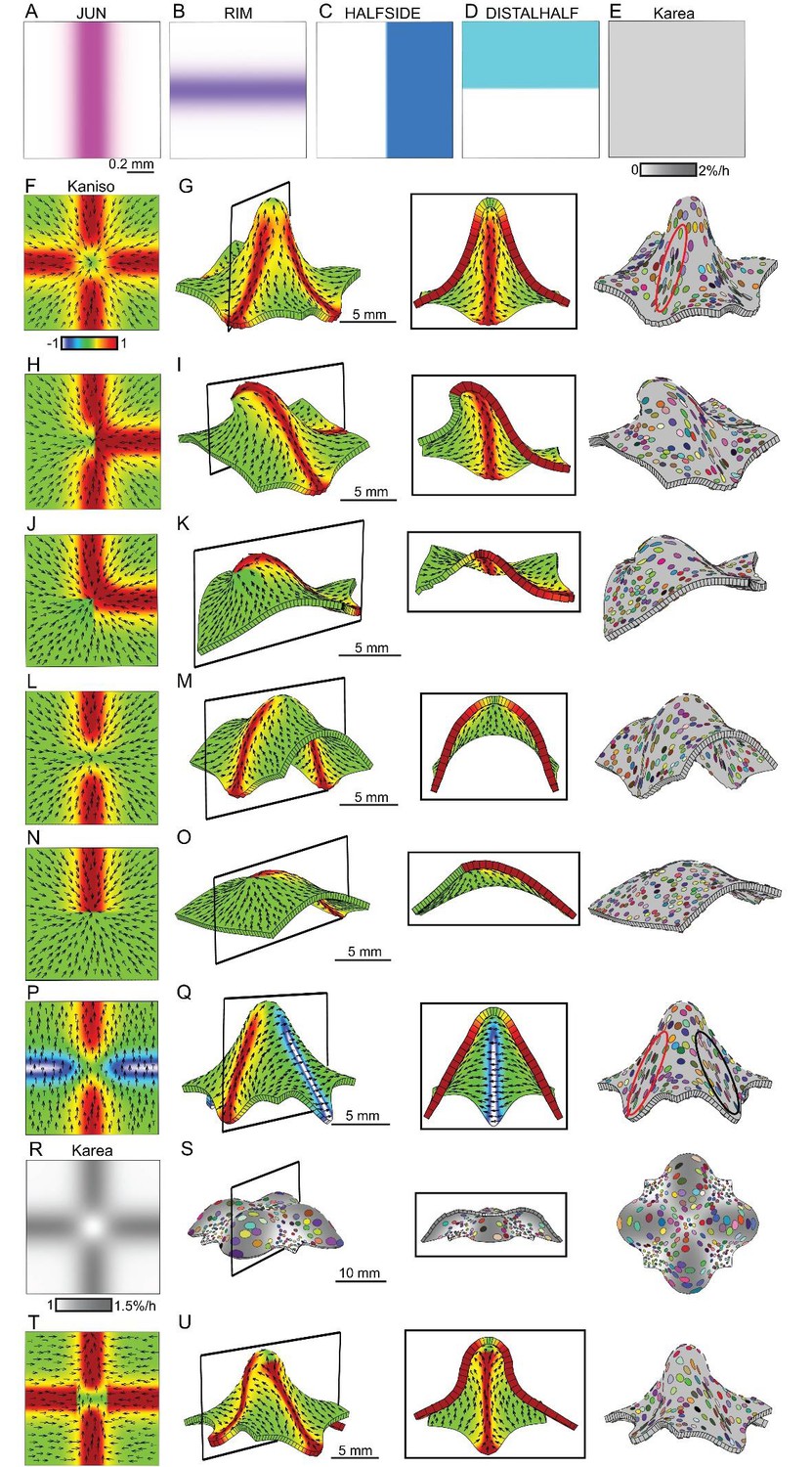
Generation of domes through orthogonal tissue conflicts.
(A–D) Expression pattern of four growth regulatory factors. JUN is expressed as a vertical domain in the middle of the canvas (A), RIM as a horizontal line in the middle of the canvas (B), HALFSIDE in the right side of the canvas (C) and DISTALHALF in the upper half of the canvas (D). In all models the Karea = (Kpar + Kper) was maintained uniform throughout the canvas (E). (F–O) Orthogonal directional conflict models. In the first example Kpar is enhanced in an orthogonal domain established by JUN and RIM but not at the intersection of these factors (F) to generate a dome with clones more elongated in the arms of the orthogonal domains (red ellipse) than in the neighbouring quadrants (G). Modifications to this orthogonal pattern generated variously shaped domes (H–O). A T-shaped pattern (H) generated an asymmetric dome (J). An L-shaped pattern (J) gave a less pronounced asymmetric dome (K), while removing both side arms of high anisotropy (L), gave a ridge with clones more elongated along it (M). Removing all arms but one gave an asymmetric ridge (N–O). (P–U) An orthogonal pattern of directional conflict in a parallel polarity field, generated by boosting Kpar by JUN while boosting Kper by RIM (P). This specified growth pattern generated an elongated dome with clones elongated parallel to the polarity along the regions of high Kpar (red ellipse in Q) and perpendicular to the polarity along the regions of high Kper (black ellipse in Q). Between these regions clones are more isodiametric (Q). Boosting isotropic growth with JUN and RIM (Karea in R) resulted on the formation of four bulges but no dome (S). An orthogonal pattern of directional conflict can also be generated with a channel of proximodistal polarity in the JUN domain, and mediolateral polarity in flanking regions (T). An orthogonal domain of high Kpar generates a wide dome (U). Kaniso = ln (Kpar /Kper). The colour scale for Kaniso is –1 to +1.
Figure 6—figure supplement 1
Combining tissue conflicts.
(A–D) Combining orthogonal direction with areal conflict, by enhancing areal growth in the orthogonal domains while inhibiting growth at the intersection (A), produced a rounded dome with protruding edges (B). A 10% growth differential between surfaces (surface conflict) can be combined with an orthogonal conflict as in Figure 1I to generate an elongated dome with a wide base (C) or with an areal conflict as in Figure 1G to produce a rounded dome (D). Kaniso = ln (Kpar /Kper) colour scale between the −1 and 1; Karea = Kpar + Kper.
Figure 7
Generation of domes by tissue conflicts through contraction and growth.
Similar shape domes to Figure 1 can be generated using a combination of contraction and growth, with overall canvas size remaining the same. (A–B) Surface conflict. Uniform isotropic specified growth for one surface (blue) and isotropic specified contraction (negative growth) for the other surface (lilac), causes an initial square (A) to deform into a dome with downward curled edges (B). (C–D) Areal conflict. Isotropic specified growth in the centre counterbalanced by contraction at the edges causes the square canvas (C) to deform into a rounded dome with circular clones which are bigger at the apex (D). (E–F) Directional conflict with a convergent polarity field. Uniformly high specified growth parallel to the polarity is counterbalanced by uniformly high specified contraction perpendicular to the polarity. The canvas deforms from an initial square (E) into a dome with elongated clones parallel to the polarity field (F). (G–H) Orthogonal directional conflict with a parallel polarity field. High specified growth parallel to the polarity in the vertical domain (red) and perpendicular to the polarity in the horizontal domain (blue) are counterbalanced by contraction perpendicular to the polarity in the vertical domain and parallel in the horizontal domain (G). A dome is generated with clones elongated parallel to the polarity in the red domain and perpendicular to the polarity in the blue domain (H). Kaniso = ln(Kpar /Kper). The colour scale for Kaniso is –1 to +1. Karea = Kpar + Kper.
Figure 8 with 2 supplements
PIN1 polarity and correlation with cell file orientation.
(A–H) Whole-mount immunolocalisation in div and wild-type ventral-lateral junctions using the antibody raised to the PIN1a peptide at 11 DAI (A–D) and 13 DAI (E–H). Left panels show confocal images of PIN1 immunolocalisation (red signal). Right panels depict the average PIN1 polarity (yellow arrows) calculated using the PinPoint software. At 11 DAI, PIN1 is expressed at the ventral-lateral petal junction (blue dashed line) just below the sinus (blue arrow) and points proximodistally towards the petal margin (white outline) in both div (A and B) and wild type (C and D). At 13 DAI, PIN1 expression extends more proximally in div (E and F) and to an ever greater extent in wild type (G and H). The PIN1 polarity in wild type has a central region of 2–3 proximodistal files (within green dashed line in G) and flanking regions with diagonal polarity deflected towards the central files (G and H). Scale bar, 10 μm. Px, proximal, Di, distal. (I and J) Confocal images of div (I) and wild-type (J) ventral-lateral junctions at 13 DAI combining the immunohybridised PIN1a antibody signal (red) with the calcofluor white cell wall signal (cyan) at different magnifications (yellow and orange boxes). When overlapping, the orientation of the cell files correlates with the pattern of cellular PIN1 polarity: proximodistal cell files have proximodistal PIN1 polarity (e.g. files marked with white dashed lines in yellow boxes) while diagonal cell files have diagonally oriented PIN1 polarity (e.g. files marked with green dashed line in yellow boxes). The region of PIN1 expression does not overlap with the region where the mediolateral growth is observed (white outlines in oranges boxes). Asterisks refer to subepidermal PIN1 signal in the vascular tissue. Scale bar (E and F), 100 μm and (G) 10 μm.
Figure 8—figure supplement 1

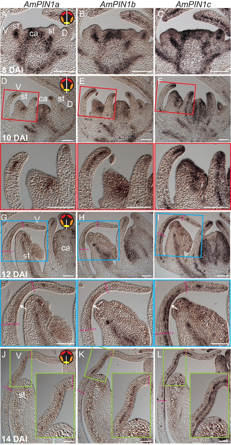
Expression patterns of AmPIN1 genes.
(A-L) Expression patterns of AmPIN1 genes at 8 DAI (A-C), 10 DAI (D-F), 12 DAI (G-I) and 14 DAI (J-L), determined by RNA in situ hybridisation of alternative sections hybridised with AmPIN1a (left panels, A, D, G, J), AmPIN1b (middle panels, B, E, H, K) and AmPIN1c (right panels, C, F, I, L) probes. The AmPIN1 genes show similar expression patterns in the vascular tissue of petal primordia (A-F), with some localised differences particularly at the tips of the petal primordia (D-F and close-ups of red boxes in respective D-F images), in particular for AmPIN1c which shows stronger epidermal expression at the petal tips. At 12 DAI, the AmPIN1 genes continue to be expressed in the vascular tissue (G-I) but are additionally detected at the epidermis of the palate and lip regions, particularly strongly for AmPIN1c (white arrows in close-ups of blue boxes in respective G-I images). At 13 DAI, the epidermal AmPIN1 expression starts to decrease (J-L) in comparison with the vascular tissue signal which continues to be similar to previous stages (close-ups of green squares in respective J-L images). The upper and lower limits of the palate and lip domains are marked by pink dashed lines. The diagram in the upper right corner of every left panel represents the orientation of the section (white line) relative to the five petals (red-dorsal, orange -lateral and yellow -ventral). V: ventral petal; D: dorsal petal; st: stamen; ca: carpel. Scale bars, 100 μm.
Figure 8—figure supplement 2
PIN1 polarity patterns in div and wild type.
(A–C) Scanning electron micrograph of a flower bud at 9 DAI, showing the dorsal (D, red shading), lateral (L, orange shading) and ventral (V, yellow shading) petals (A). Confocal images of PIN1 section-immuno (red signal) in calcofluor stained petal tissue (cyan signal) with a longitudinal section (B, position of section indicated by blue line in A) and a frontal section (C, position of section indicated by magenta line in A). The PIN1 signal is strong in the epidermis, where polarity points proximodistally towards the tip of the petal (white arrows in petal tip, yellow box inset in B) and in the internal tissues where the vascular tissues starts to develop. This PIN1 pattern is confirmed in a frontal section, where the epidermal PIN1 converges towards the most distal cells at the tip of the petal while internally, the PIN1 polarity in the sub-epidermal cells points towards the developing vascular strand (white arrows in green box inset of C). White line in B-C marks the petal edge. Px, proximal, Di, distal. Scale bar (A, B and C), 100 μm. Scale bar (D and E), 10 μm. (D-I) Confocal images of PIN1 whole-mount immuno in div (D, F and H) and wild-type (E, G and I) ventral-lateral sinus at 11 DAI (D and E), 13 DAI (F and G) and 15 DAI (H and I). Polarity of the PIN1 subcellular signal was estimated using the PinPoint software and is labelled with white arrow heads. Initially, PIN1 expression (red) is observed at the petal sinus and its cellular polarity is largely proximodistal at the sinus and proximomarginal along the marginal cells pointing towards the tips of the petals in both div and wild-type (D and E). Although the expression expands in div, its polarity pattern is maintained proximodistal (F). In wild type the extended PIN1 region is larger than in div (compare G to F) and is oriented proximodistally along the petal junction (3–4 central files) (files within green dashed line in H and zoomed-in image in blue box) while either side of this junction, polarity points diagonally, towards the central files and nearby sinus (G). At day 15, PIN1 expression at the sinus becomes restricted to the petal margins, both in div and wild-type (H and I). Scale bar, 10 μm. (J and K) PIN1 whole-mount immuno in wild-type lateral-dorsal sinus at 11 DAI (J) and 13 DAI (K). PIN1 signal is restricted to the sinus region where it shows a proximodistal polarity in the margin cells (next to white line) and a proximomarginal polarity in the cells adjacent to the marginal cells (J). The PIN1 expression at the lateral-dorsal junction is transient, as at 13 DAI no signal is observed around the sinus region (blue arrow) (K). Vascular strands have strong PIN1 signal (strands marked with asterisk). Scale bar, 10 μm. (L) Images of cells showing PIN1 in red (leftmost column), calcofluor cell wall staining in blue (second column), and composite image of PIN1 and calcofluor for use with the PinPoint software (third column). Sample cell segmentations are shown in yellow and polarity directions calculated from PinPoint software are indicated with yellow arrows (rightmost column).
Figure 9 with 1 supplement

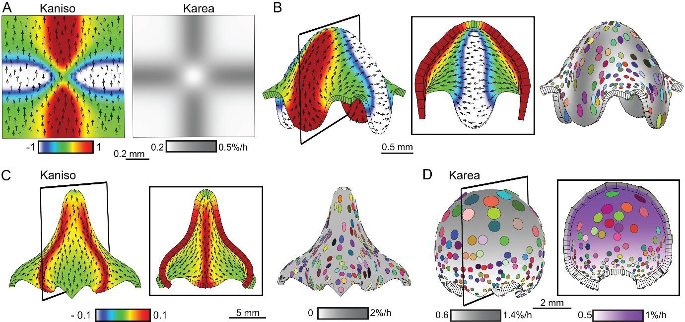
Tissue-level model of div corolla development.
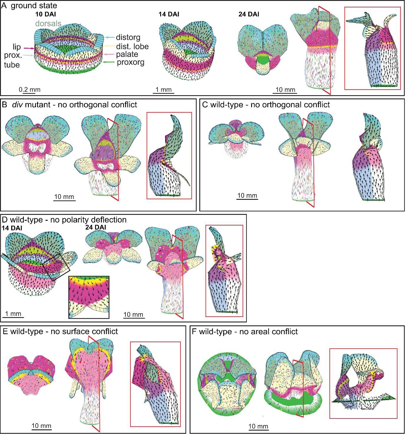
(A–F) Modelling formation of div domes. (A) The initial shape represents a strip of tissue at the tube to lobe boundary, from which the domes develop (Figure 3H–J). The strip is slightly curved to represent the initial petal shape, as shown in the side view of the canvas thickness (Side). During the setup phase, several identity factors are established in domains along three different axes: (1) dorsoventral – sRAD which grades into the lateral petals from the dorsal petals, (2) proximodistal - LIP, PLT, RIM and BRIM and (3) mediolateral - LAT at petal junctions, and MED in the midvein region. (B) These factors interact combinatorially to control the specified rates of growth parallel (Kpar) and perpendicular (Kper) to the proximodistal polarity field (black arrows). Growth is initially higher in Kpar than in Kper (Kaniso). (C) Surface conflict introduced by differential growth at the rim. Kapar is specified Kpar on the abaxial surface of the canvas, whereas Kbpar is specified Kpar on the adaxial surface. The lower value of Kapar relative to Kbpar in rim region will lead to bending of the canvas at the rim. (D) Growth rate is higher in the LIPDISTAL region (see darker grey in the distal region of the canvas), and inhibited at the hinge region by sRAD (lighter shade of grey at the lateral edges of canvas. (E) The above pattern of growth produces a strip with short hinge region at 11.5 DAI just before the time of repatterning. At 12 DAI, an orthogonal pattern of directional conflict is introduced. Kpar is enhanced by LAT around the petal junctions (white lines) and inhibited by RIM, while Kper is enhanced by RIM and inhibited by MED and LAT (the orthogonal pattern of anisotropy is marked by dashed white lines for the lateral-ventral junctions, and red dashed lines for the lateral-dorsal junction). (F) Growth following repatterning leads to a shape at 24 DAI similar to the div lower lip, with two domes at the foci region and an extended asymmetric lip (left panel shows Kaniso, while right panel shows the LIP and PLT regional factors and virtual clones). Virtual clones are predominantly elongated along the proximodistal domain except in the RIM region where clones are mediolateral oriented. (G–J) Evaluating the contribution of growth conflicts to the shape of the div model. (G) Removal of surface conflict produced a similar shape as in F but the out-of-plane deformations protrude towards the abaxial side instead of the adaxial side (left panel shows Kaniso, while right panel shows the LIP and PLT regional factors and virtual clones). (H) Removal of areal conflict, by normalising the areal growth across the canvas while maintaining the anisotropy, generated a curved canvas with long hinge region and abaxial protruding foci. (I) Removing all directional conflict by setting polariser to zero, so that all growth is isotropic, resulted in a curved narrow strip with slight bulges at the region of the high growth in the div (dark grey areas around the petals junctions. (J) Removing only the orthogonal directional conflict, resulted in a canvas with a broad flat lip and a uniform bend at the RIM without domes. (K) Incorporating the above div patterns of areal, surface and directional conflict into the full Snapdragon model produced a div mutant corolla with an extended lip (dark pink), short palate (pink) and two domes at the RIM (yellow) centred on the foci. Canvas shown at 14 DAI and maturity (24 DAI). Kaniso = ln(Kpar /Kper). The colour scale for Kaniso is –1 to +1. Karea = Kpar + Kper.
Figure 9—figure supplement 1
Virtual mutants in the Snapdragon model.
(A) Ground-state Snapdragon corolla model, based on the published model but stripped of the genetic interaction that modulate the growth rates and orientations across the lip and palate regions of lower corolla. At 10 DAI (left panel), the proximodistal polarity field is established by proxorg (green) and distorg (blue) and the polariser gradient is represented by the black arrows. The identity factors are defined throughout the canvas and control the rates of growth parallel and perpendicular to the polarity field. The different identity factors are established along three different axes, but here only the dorsoventral and the proximodistal axis are depicted. The dorsoventral axis is indicated by the darker shading of the dorsal petals. The proximodistal axis comprises of four regions: the distal lobe (dist. lobe - light yellow), the lip (dark pink), the rim (yellow), the palate (light pink) and the tube (white). The lower corolla at 14 DAI does not exhibit out-of-plane deformations and grows straight (middle panel). The lower corolla shape is maintained until maturity (24 DAI panels, with top and front views marked with virtual clones in the left and middle panels, respectively, and a mid-longitudinal section in the right panel). (B) div mutant model without the orthogonal conflict (with a front view and side marked with virtual clones in the left panel and middle panel, and a mid-longitudinal marked with polarity in the right panel). (C) Wild-type model without the orthogonal conflict (with a front view and side marked with virtual clones in the left panel and middle panel, and a mid-longitudinal marked with polarity in the right panel). (D) Wild-type model at the repatterning stage without the deflection of the polarity at the sinus (14 DAI panel, compare black arrow pattern in black box of F with D). The shape at maturity is depicted in the 24 DAI panels (with top and front views marked with virtual clones in the left and middle panels, respectively, and a mid-longitudinal section in the right panel). (E-F) Removing tissues conflicts. Wild-type shape when the surface conflict is removed (E). Wild-type shape when the areal conflict is removed (F). Red square in mid-longitudinal section indicates section plane in front view.
Figure 10

Tissue-level model of wild-type corolla development.
(A–J) Modelling of the wild-type wedge. (A) The regional identities are similar to those in div (Figure 9A) with the addition of the graded DIV expression (yellow shading) and a region, SEC, between the midvein and petal junctions (bottom panel). (B) Growth is initially higher in Kpar than in Kper (Kaniso). (C) DIV inhibits Kapar at the ventral-lateral junctions (whiter domain in Kapar), while the RIM region is kept short by DIV inhibiting Kpar slightly on both surfaces. (D) Growth is boosted in the region of the proximal lip and the palate (see darker grey regions in Karea). (E) The above pattern of growth results in a taller strip, compared to div, at 11.5 DAI (compare with Figure 9E). At 12 DAI (repatterning stage), DIV promotes Kper in combination with SEC and LIP, extending the region of high mediolateral growth (Kaniso, modified orthogonal pattern indicated with white dashed lines). DIV also activates expression of a minus organiser at the sinus (blue arrows), deflecting the polarity field towards it. (F) The above specified pattern of growth leads to a shape and pattern of clone orientations similar to that of Figure 2E (left panel shows Kaniso while right panel shows the LIP and PLT regional factors and virtual clones). (G–J) Evaluating the contribution of growth conflicts to the shape of the wild-type wedge models. (G) Removal of surface conflict produced a similar shape as in F but the out-of-plane deformations protrude towards the abaxial side instead of the adaxial side. (H) Removing areal conflict generated a small wedge with protruding foci and a long hinge region. (I) Removing all directional conflict, resulted in a narrow strip with big bulges at the lateral petal which would normally form the flanks of the wedge. (J) Removing only the orthogonal conflict resulted in a shape with a long palate, sharp bend at the rim (left and middle panel) and a narrow lip (side view in right panel). (K) Incorporating the above growth patterns of areal, surface and directional conflict into the full Snapdragon model produced a closed mouth wild-type corolla, with an extended palate, a ridge at the rim and a steep lip. Canvas shown at 14 DAI and maturity (24 DAI). The region of deflection of polarity induced at the repatterning stage is shown enlarged at 14 DAI. Regions highlighted are lip (dark pink), palate (pink) and rim (yellow). Kaniso = ln(Kpar /Kper). The colour scale for Kaniso is –1 to +1. Karea = Kpar + Kper.
Figure 11
Tissue-level models of dorsoventral mutants.
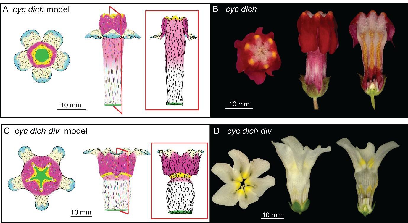
Comparison between corolla shapes of virtual mutants generated by removing gene activities from the tissue-level model (A, C) and corresponding phenotypes of real corollas (B, D). Double mutant cyc dich (A,B) and triple mutant cyc dich div (C,D) are shown. For each panel, corollas are viewed from top (left), side (middle) and in longitudinal mid-section (right, position of section for the virtual corollas indicated by red line in middle panel). For the virtual mutants, regions highlighted are lip (dark pink), palate (pink) and rim (yellow).
Figure 12
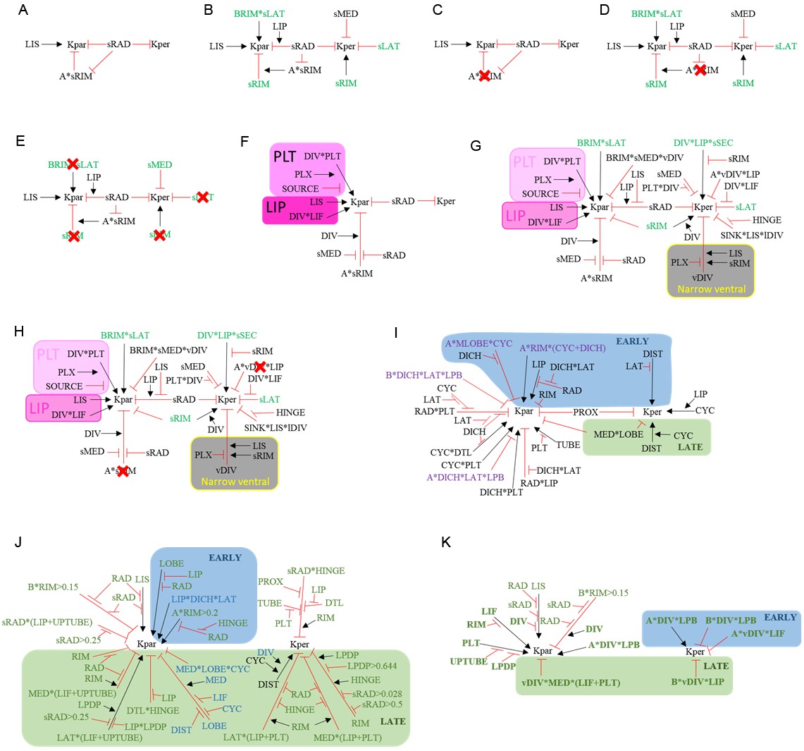
Summaries of growth regulatory networks (KRNs) used in models See materials and methods for full explanation.
(A) Phase I of div domes. (B) Phase II of div domes. (C) Phase I of div domes with no surface conflict. (D) Phase II of div domes with no surface conflict. (E) Phase II of div domes with no orthogonal conflict. (F) Phase I of wild-type wedge. (G) Phase II of wild-type wedge. (H) Phase II of wild-type wedge with no surface conflict. (I) Ground state of full corolla model. (J) div mutant full corolla model showing new interactions (green) and modified interactions (blue). (K) Wild-type full corolla model showing only DIV-dependent interactions (green and bold).
Videos
Video 1
Isotropic growth model as in Figure 1B.
The size of the canvas is not rescale to better show the increase in canvas size.
Video 2
Anisotropic growth model as in Figure 1D.
The size of the canvas is not rescale to better show the increase in canvas size.
Video 3
Surface conflict model as in Figure 1F.
Size of canvas is rescaled to better visualise the deformation of the canvas.
Video 4
Areal conflict model as in Figure 1H.
Size of canvas is rescaled to better visualise the deformation of the canvas.
Video 5
Directional conflict as in Figure 1J.
Size of canvas is rescaled to better visualise the deformation of the canvas.
Video 6
Orthogonal directional conflict model as in Figure 6G.
Size of canvas is rescaled to better visualise the deformation of the canvas.
Video 7
T-shaped orthogonal directional conflict model as in Figure 6I.
Size of canvas is rescaled to better visualise the deformation of the canvas.
Video 8
L-shaped orthogonal directional conflict model as in Figure 6K.
Size of canvas is rescaled to better visualise the deformation of the canvas.
Video 9
I-shaped directional conflict model as in Figure 6M.
Size of canvas is rescaled to better visualise the deformation of the canvas.
Video 10
One arm directional conflict model as in Figure 6O.
Size of canvas is rescaled to better visualise the deformation of the canvas.
Video 11
Orthogonal directional conflict model as in Figure 6Q.
Size of canvas is rescaled to better visualise the deformation of the canvas.
Video 12
Orthogonal areal conflict model as in Figure 6S.
Size of canvas is rescaled to better visualise the deformation of the canvas.
Video 13
Orthogonal directional conflict model as in Figure 6U.
Size of canvas is rescaled to better visualise the deformation of the canvas.
Video 14
div domes model as in Figure 9F.
Size of canvas is rescaled to better visualise the deformation of the canvas.
Video 15
div domes model without surface conflict as in Figure 9G.
Size of canvas is rescaled to better visualise the deformation of the canvas.
Video 16
div domes model without areal conflict as in Figure 9H.
Size of canvas is rescaled to better visualise the deformation of the canvas.
Video 17
div domes model without directional conflict as in Figure 9I.
Size of canvas is rescaled to better visualise the deformation of the canvas.
Video 18
div domes model without orthogonal directional conflict as in Figure 9J.
Size of canvas is rescaled to better visualise the deformation of the canvas.
Video 19
div full Snapdragon model as in Figure 9K.
Size of canvas is rescaled to better visualise the deformation of the canvas.
Video 20
Wild-type wedge model as in Figure 10F.
Size of canvas is rescaled to better visualise the deformation of the canvas.
Video 21
Wild-type wedge model without surface conflict as in Figure 10G.
Size of canvas is rescaled to better visualise the deformation of the canvas.
Video 22
Wild-type wedge model without areal conflict as in Figure 10H.
Size of canvas is rescaled to better visualise the deformation of the canvas.
Video 23
Wild-type wedge model without directional conflict as in Figure 10I.
Size of canvas is rescaled to better visualise the deformation of the canvas.
Video 24
Wild-type wedge model without orthogonal directional conflict as in Figure 10J.
Size of canvas is rescaled to better visualise the deformation of the canvas.
Video 25
Wild-type full Snapdragon model as in Figure 10K.
Size of canvas is rescale to better visualise the deformation of the canvas.
Video 26
cyc dich double mutant model as in Figure 11A.
Size of canvas is rescale to better visualise the deformation of the canvas.
Video 27
cyc dich div triple mutant model as in Figure 11C.
Size of canvas is rescale to better visualise the deformation of the canvas.
Download links
A two-part list of links to download the article, or parts of the article, in various formats.
Downloads (link to download the article as PDF)
Open citations (links to open the citations from this article in various online reference manager services)
Cite this article (links to download the citations from this article in formats compatible with various reference manager tools)
Generation of shape complexity through tissue conflict resolution
eLife 6:e20156.
https://doi.org/10.7554/eLife.20156


