Transformation of spatiotemporal dynamics in the macaque vestibular system from otolith afferents to cortex
- Baylor College of Medicine, United States
- Zhongshan Opthalmic Center, Sun Yat-sen University, China
- Zhejiang University, China
- University of Rochester, United States
Figures
Figure 1
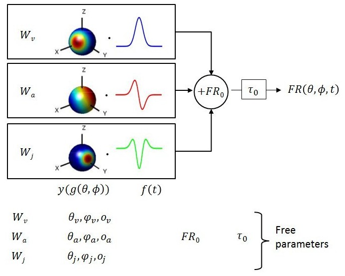
Schematic of model with velocity, acceleration and jerk components.
The fitted function, is the sum of three components, each consisting of a weight , a 3D spatial tuning function ( represented on a sphere) and a temporal response profile (), scaled and multiplied together. Spatial tuning functions illustrate that preferred directions need not be identical for each temporal component.
Figure 2
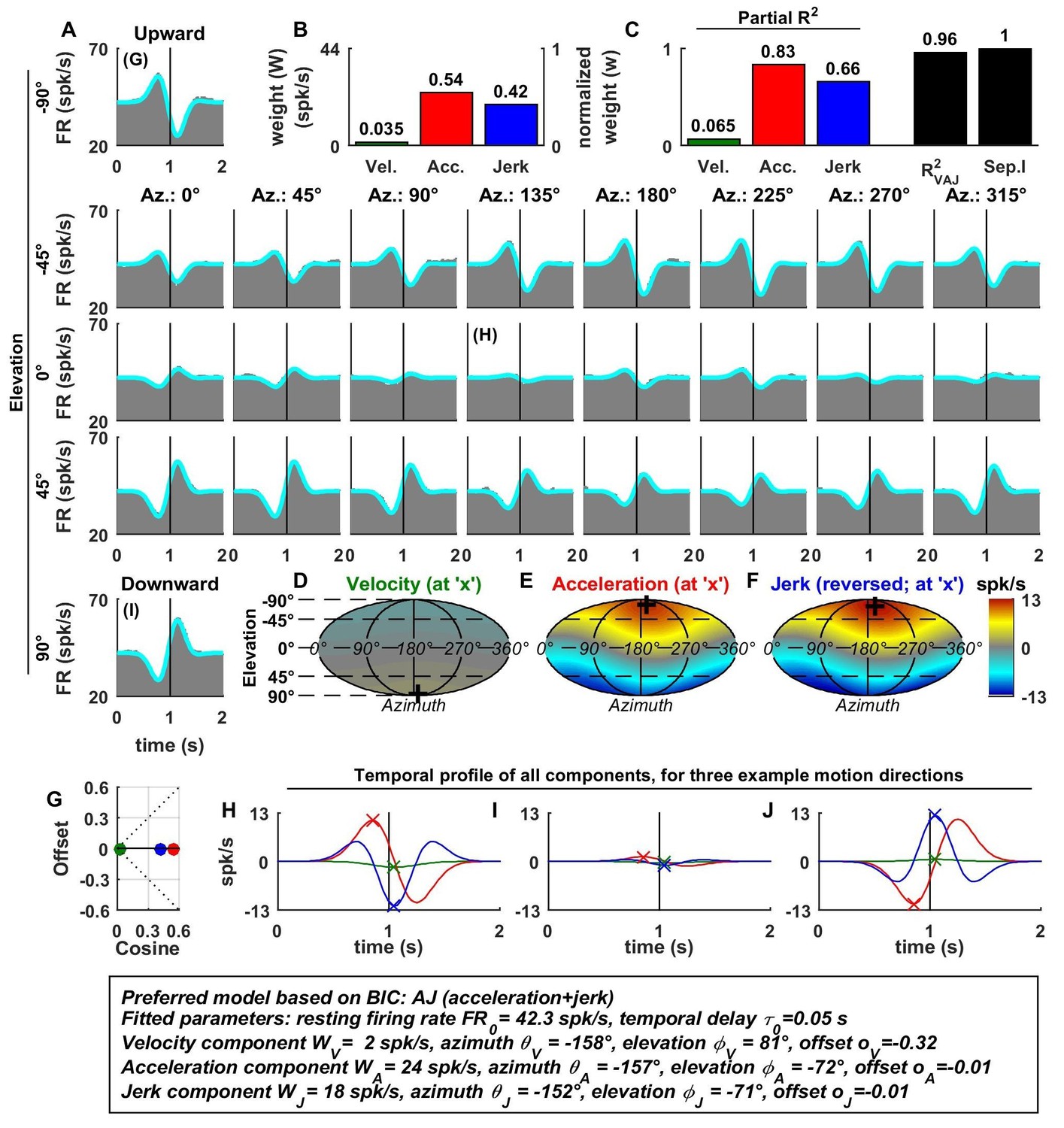
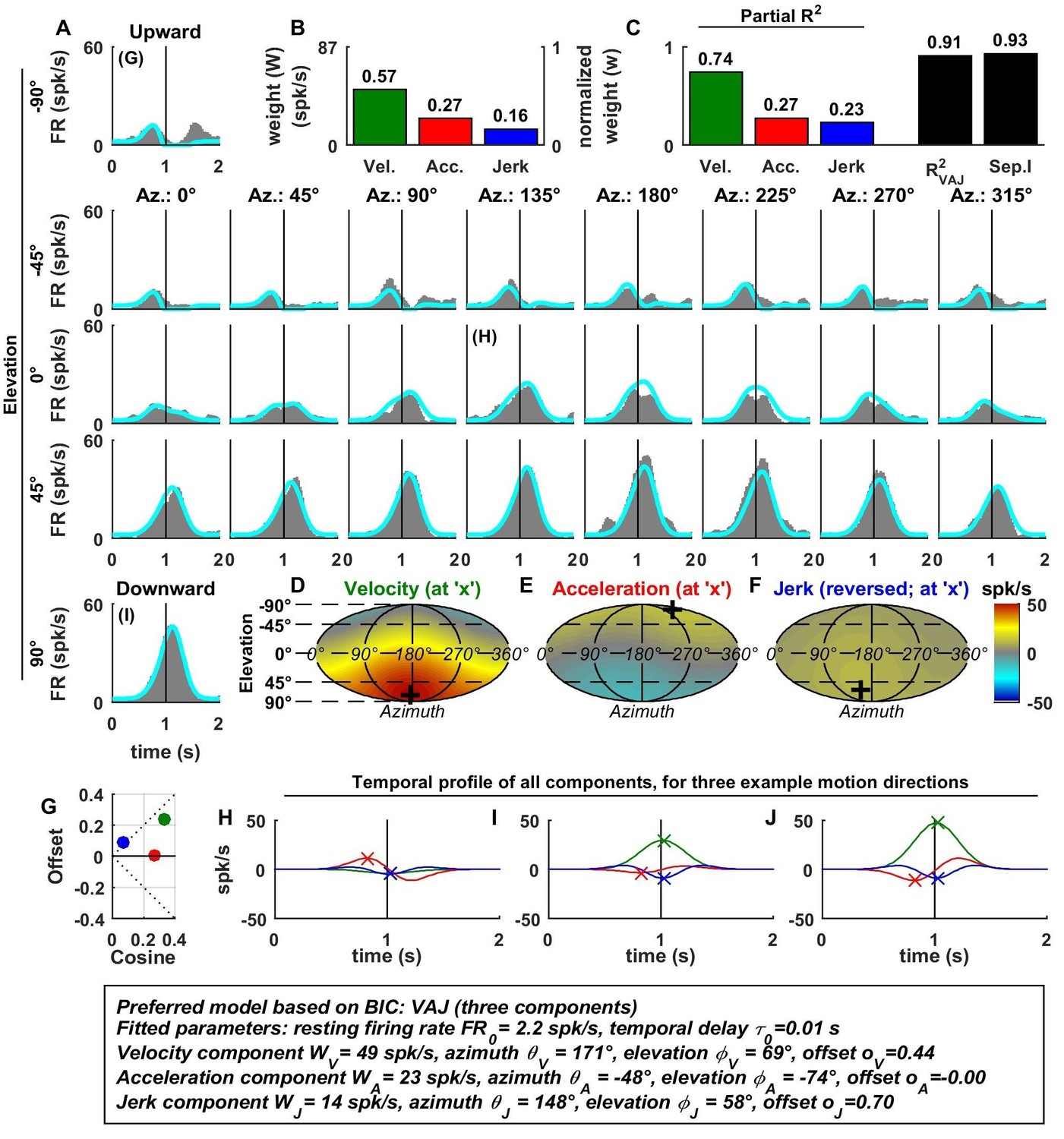
Spatio-temporal tuning of an example otolith afferent that was best fit by the AJ model.
(A) PSTHs (gray) and model fits (cyan) for each of the 26 stimulus directions, defined by the corresponding (azimuth, elevation) angles. The vertical lines at t = 1s represent the timing of peak stimulus velocity. (B) Component weights for the fit of the VAJ model (left axis: raw weight in spikes/s, right axis: normalized weights, such that their sum = 1). (C) Partial R2 of the three components, representing their contribution to the cell’s firing; R2VAJ: goodness of fit of the full VAJ model; Sep.I: separability index, indicating how well the cell can be modeled using the same spatial tuning function for all three temporal response components (see Materials and methods). (D–F) Color intensity plots of the spatial tuning of velocity, acceleration and jerk components, respectively. For illustrative purposes, the sensitivities to velocity, acceleration and jerk, are multiplied by the peak amplitude of the respective temporal profiles such that the three spatial tuning functions are expressed in spikes/s. Therefore, (D) represents the contribution of the velocity component at the time of peak velocity (plus the delay ); (E) represents the contribution of acceleration at the time of peak acceleration (plus ); (F) represents the contribution of jerk at the time of peak jerk (plus ). The crosses in (D–F) indicate the preferred direction of each component. Note that a positive sensitivity to jerk (for upward jerk in this cell) corresponds to a negative response at t = 0 (see G) since jerk is negative at that time. (G) Offset () versus cosine tuning amplitude () of the three temporal components. (H–J) Temporal profiles of the three components [velocity (green), acceleration (red) and jerk (blue) scaled by the respective component weight] for the stimulus directions indicated in A. The x marks illustrate the times for which the spatial tuning in D-F has been plotted.
Figure 3 with 6 supplements

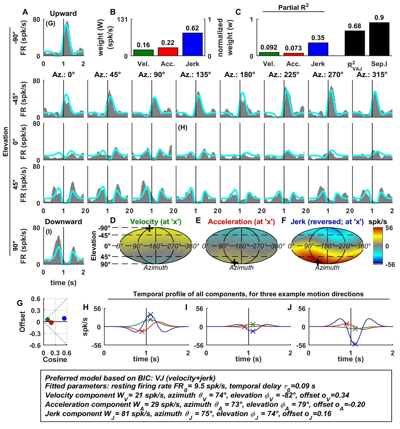
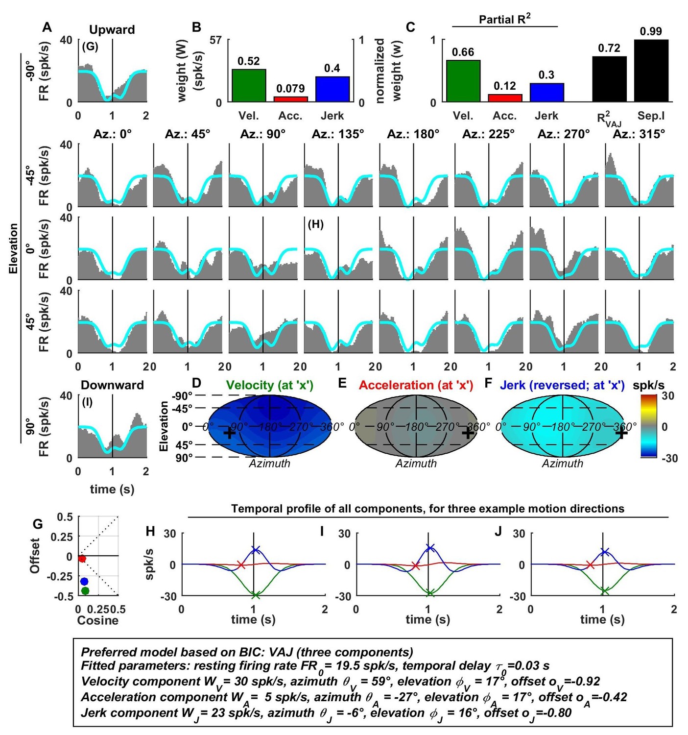
Spatio-temporal tuning and VAJ model fit for an example VN cell.
Format as in Figure 2. Note that the neuron responds to translation in all directions (A), with different temporal response profiles that result from velocity, acceleration and jerk components having different spatial tuning (D–F), thus resulting in a relatively small separability index (C). Note also that the cell is characterized by nearly uniform tuning to velocity and jerk (D,F), which is modeled as a high offset combined with a relatively small cosine tuning amplitude (G, green and blue). Additional example cells are presented in Figure 3—figure supplements 1–6.
Figure 3—figure supplement 1

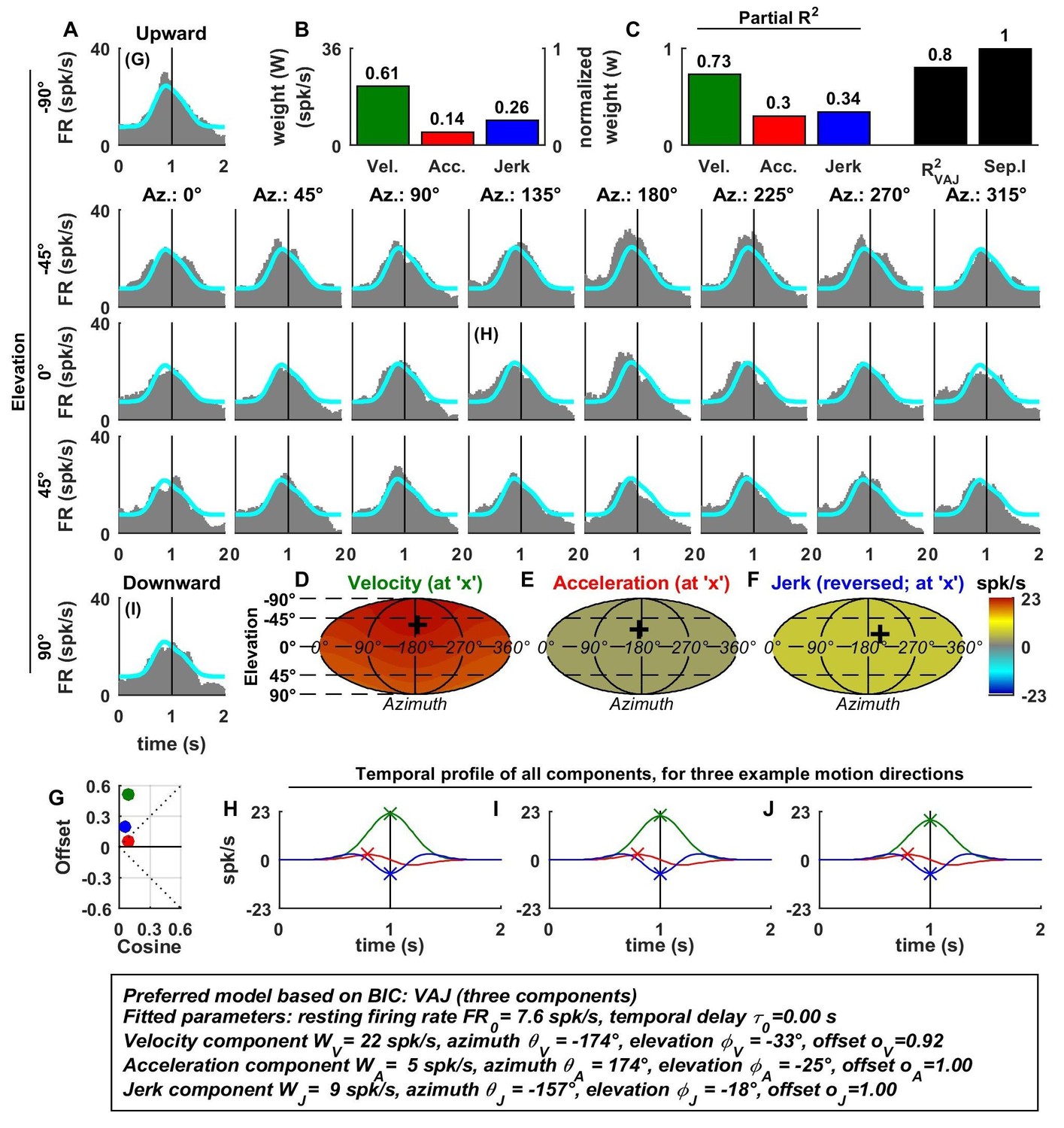
Spatio-temporal tuning of an example CN cell.
(A–J) Format as in Figures 2 and 3. The cell's firing increases during motion in all directions due to its nearly uniform tuning to velocity and jerk (D,F), which is modeled as a low cosine tuning amplitude and a high offset (G, green and blue). Note that the cell’s PSTH varies as a function of motion direction due to the cell's cosine tuning to acceleration (E, low offset in G, red)– despite very broad non-linear tuning to velocity and jerk. This pattern represents the most frequently encountered type of central neuron. Also note that the separability index was high, despite the strongly non-cosine tuning of velocity and jerk. This is because the spatial tuning of velocity and jerk is often very broad, and the separability index is a measure of the tuning similarity of the different temporal components. Thus, a separability index close to one does not necessarily imply cosine (afferent-like) spatial tuning.
Figure 3—figure supplement 2
Spatio-temporal tuning of an example PIVC cell, exhibiting a strong, cosine-like response to jerk.
https://doi.org/10.7554/eLife.20787.007
Figure 3—figure supplement 3
Spatio-temporal tuning of an example VPS cell, whose temporal response is dominated by velocity, exhibiting a nearly uniform response to motion in all directions (D; high offset and low cosine tuning amplitude in G, green) and a high separability index (=1), despite strongly non-linear responsiveness.
https://doi.org/10.7554/eLife.20787.008
Figure 3—figure supplement 4
Spatio-temporal tuning of an example MSTd cell, whose temporal response is dominated by velocity.
This cell exhibits both cosine tuning and offset response to velocity (G, green), resulting in relatively narrow velocity tuning characterized by a strong positive response to downward motion but little response to motion in other directions. Format as in Figures 2 and 3.
Figure 3—figure supplement 5
Spatio-temporal tuning of an example VIP cell, exhibiting a decrease in firing in response to motion in all directions due to a uniform negative tuning to velocity and jerk.
https://doi.org/10.7554/eLife.20787.010
Figure 3—figure supplement 6

Spatio-temporal tuning of an example FEF cell, exhibiting a narrowly tuned response to upward directions, consisting of mostly velocity and acceleration components.
The response is fit with cosine tuning and a small offset (note that the fitted function always includes a rectification, such that the cell is silent during downward motion). Format as in Figures 2 and 3.
Figure 4 with 1 supplement
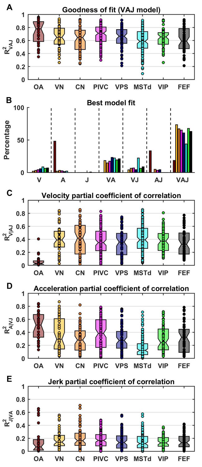
Summary of model fits.
(A) Distribution of R2VAJ values for each brain area. The boxes represent the median (center of the notch) and lower and upper quartiles of the population. Two medians are different at 5% level if the notches do not overlap. Individual data points are represented by circles. (B) Percentage of best model fits based on BIC. (C–E) Partial correlation coefficients of each of the three components, which reflect how much variance is accounted for by adding that component to the joint model of the other two components. Comparisons with model fits using an exponential spatial non-linearity function are shown in in Figure 4—figure supplement 1.
Figure 4—figure supplement 1

Fitting performance using an exponential spatial non-linearity function.
We fitted neuronal responses with an extension of the VAJ model in which the spatial non-linearity function is an exponential , as in Chen et al. (2011c). This function was normalized between −1 and 1, which reduced it to two free parameters, and therefore, the extended VAJ model had 17 free parameters. Fit quality was measured by R2VAJ (here referred to as R2exponential for the extended VAJ model and R2affine for the model used in the rest of the study, where is an affine function). (A) As expected, the extended VAJ model produced better fits (i.e., R2exponential > R2affine). However, the performance improvement was modest, as indicated by the ratio R2affine / R2exponential. This ratio was close to one for the majority of neurons; its median value was 0.97, and it was greater than 0.9 for 91% of the cells. (B) For a few cells (n = 6, 1%), the ratio was less than 0.8. However, R2exponential was also low (<0.6) for these cells. This indicates that these cells were poorly fit (with typically low and noisy responses), such that the extended model was prone to overfitting. We conclude that the extended model provides little quantitative benefit compared to its increased complexity; thus, we adopted the simpler affine model in this study.
Figure 5

Summary of model fits for otolith afferents.
(A) Difference in CV* between afferents that respond to acceleration only (‘A’) or acceleration, jerk and optionally velocity (‘AJ’ and ‘VAJ’). (B–C) Raw and normalized weights for velocity, acceleration and jerk are plotted as a function of CV*. Filled symbols, ‘A’ afferents; open symbols: ‘AJ’ and ‘VAJ’ afferents. Note that weights for each OA were taken from the VAJ model such that all cells could be included in these plots. Solid lines: statistically significant (p<10−2) type I regression lines. Broken lines: non-significant (p>0.05) regression lines. (D) The absolute difference between the 3D preferred directions of component pairs (A–J, V–A, V–J) plotted versus CV*. Here, angular differences are included only when both response components were significant for each cell. Symbols and lines as in B,C. Because A and J components were nearly aligned (black symbols), V-A (red) and V-J (blue) angular differences were similar for each cell.
Figure 6
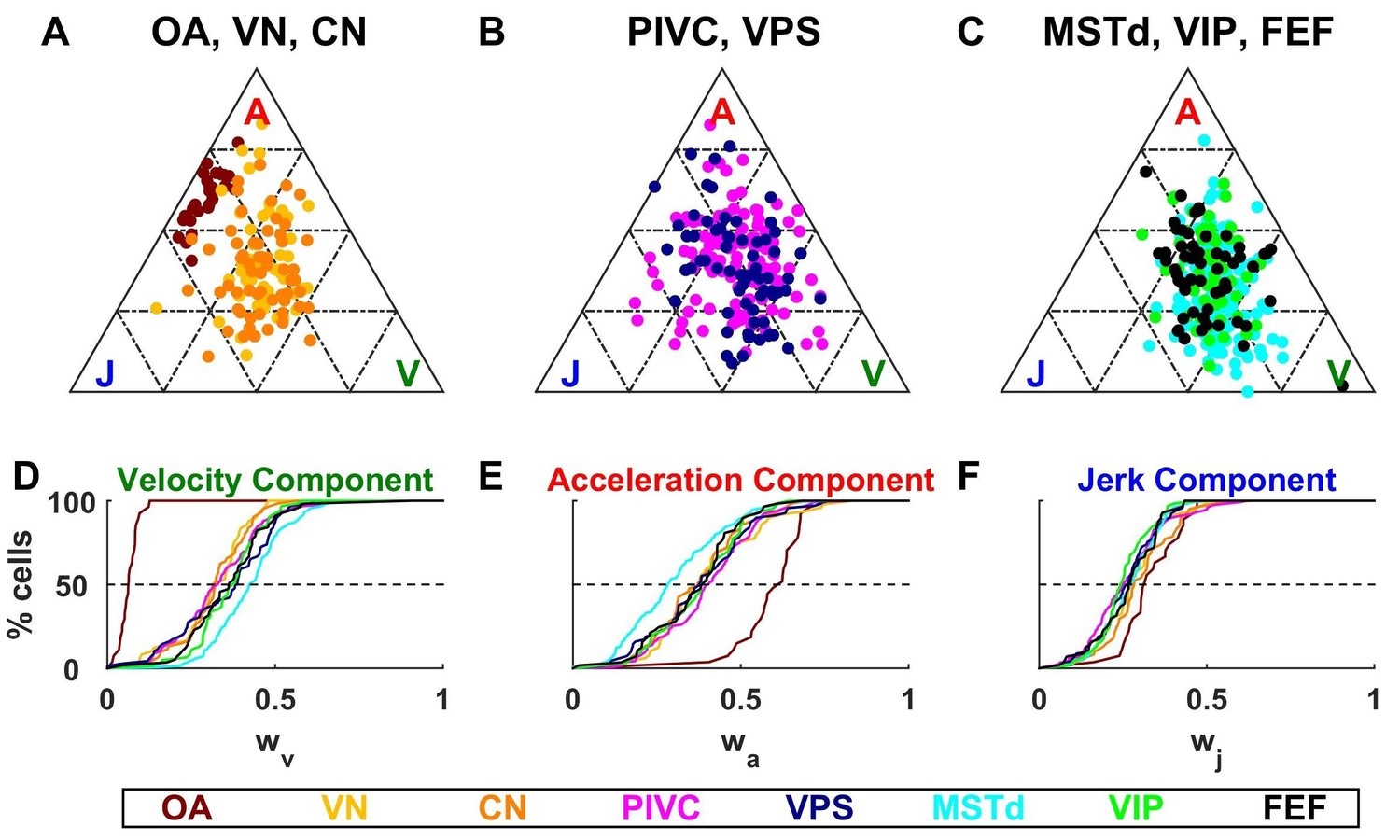
Dynamic components weights.
(A–C) Ternary plots summarizing normalized weights for the acceleration, velocity and jerk components of VAJ model fits. Each data point represents the normalized velocity, acceleration and jerk weights for a single cell, color coded by brain area. (D–F) Cumulative distributions of normalized velocity (D), acceleration (E) and jerk (F) weights. Note the similarity in normalized velocity and acceleration weights across all central brain areas.
Figure 7 with 1 supplement

Comparison of preferred directions across dynamic components.
(A) Distribution of the separability index across brain areas. (B–D) Summary of the angular difference between preferred directions of component pairs. The distribution of angles across the population is color-coded (red/yellow: aligned; green/cyan: opposite; grey: orthogonal). The ‘sum’ bar represents the distribution across all central brain areas (VN to FEF). For each comparison, only cells for which both components had significant spatial tuning have been considered (i.e. single-component best fits have not been included at all, whereas 2-component best fits have only been included in only one plot). The distribution H1 represents the expected distribution if directions are distributed randomly on a sphere, in which case orthogonal pairs (e.g. from 85° to 95°) are more likely to occur than aligned or opposite pairs (e.g. from 0° to 10°). The distribution H2 assumes only ‘aligned’ responses (like the A-J components of OAs). Bold/italic labels indicate distributions that are/are not significantly different from H1 (top) (Kolomogorov-Smirnov Test; p-values indicated in Table 3). Distributions of the preferred direction of each dynamic component are shown in Figure 7—figure supplement 1.
Figure 7—figure supplement 1

Distributions of the PD of each dynamic component.
The PDs of all cells with significant tuning are represented in spherical coordinates (azimuth , elevation ) that are projected on a plane using an equal-area Mollweide projection (a uniform distribution on a sphere corresponds to a uniform distribution on the Mollweide plane). The uniformity of PDs was tested by computing a 3D Rayleigh vector R (equal to the average of ) across neurons, for each region and each component. The observed R values were compared to a distribution P(R|H0) (under the hypothesis H0 that PD are distributed uniformly) that was estimated by drawing n directions uniformly (where n is the number of neurons), computing the corresponding R values, and repeating the operation 1000 times. We found that no component was significantly different from uniform (at p=0.01, corresponding to p=0.2 with Bonferroni correction).
Figure 8
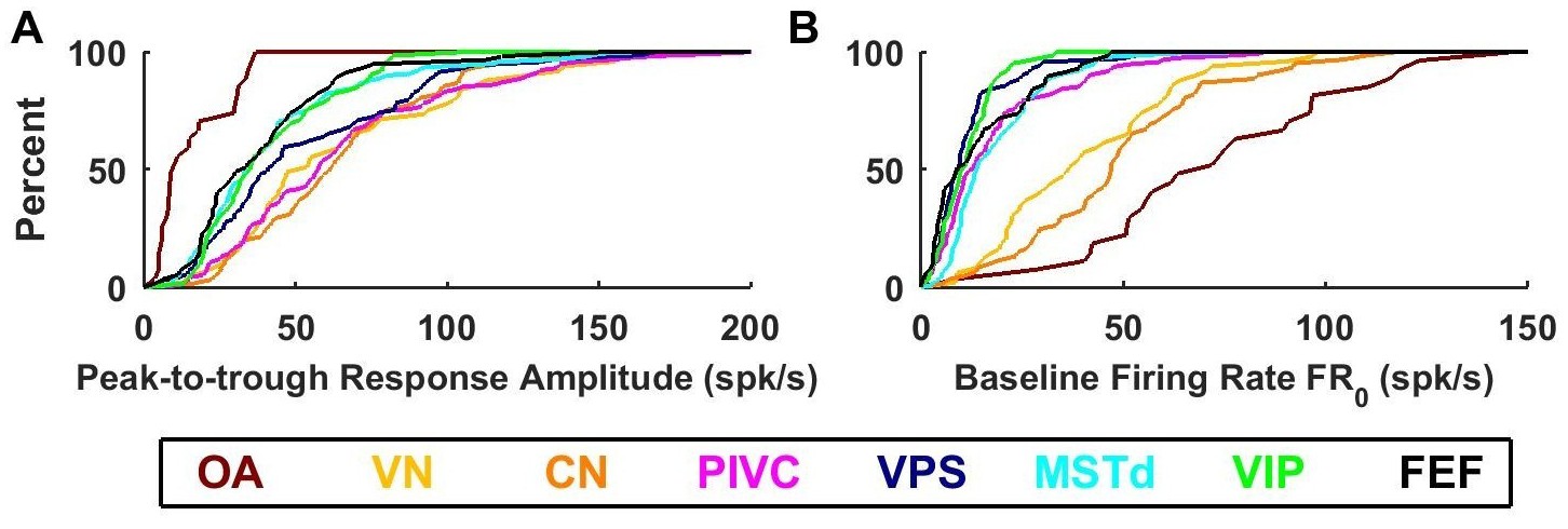
Summary of response amplitude and baseline firing rate parameters.
Cumulative distributions of (A) peak-to-trough response amplitude (maximum across all directions), and (B) baseline firing rate (). OA: otolith afferents (brown); VN: vestibular nuclei (yellow); CN: cerebellar nuclei (orange); PIVC: parietoinsular vestibular cortex (red); VPS: visual posterior sylvian (blue); MSTd: dorsal medial superior temporal area (cyan); VIP: central intraparietal area (green). FEF: frontal eye fields (black).
Figure 9 with 1 supplement
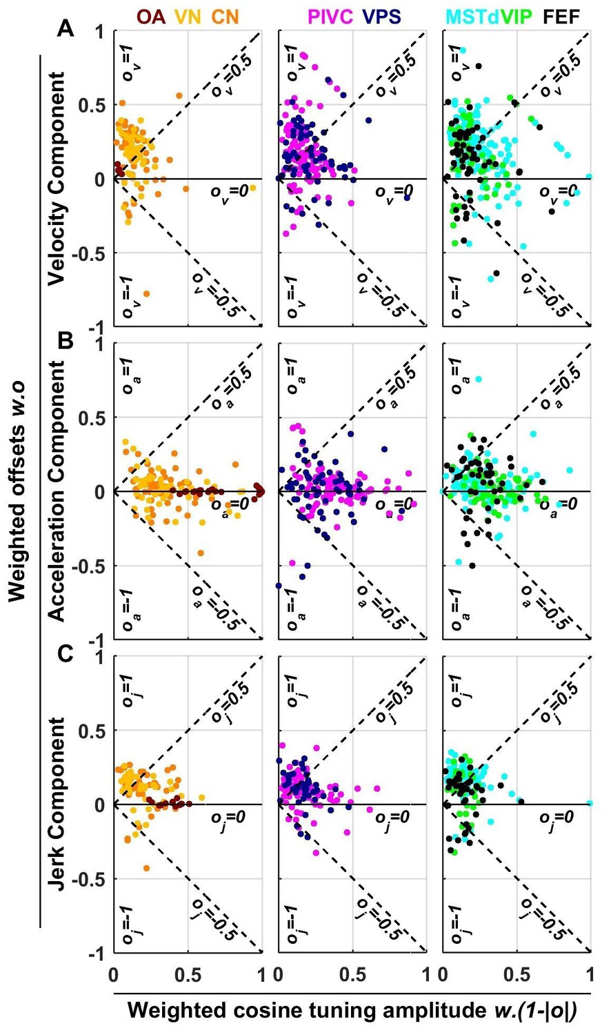
Summary of spatial tuning non-linearity for (A) velocity, (B) acceleration and (C) jerk.
The spatial tuning curves are modeled by adding an offset (, respectively) to a cosine-tuned response , i.e., (the curves follow similar forms). The relative amplitudes of the response to velocity, acceleration and jerk depend on the weights . Thus, the weighted cosine-tuned response components (abscissa) are: , and the weighted offset response components are: (ordinate). Purely cosine-tuned cells have zero offset (, ), while cells with positive or negative omnidirectional responses have a large offset and little modulation (, for positive responses, or for negative responses). Distributions of the offset parameters are shown in Figure 9—figure supplement 1.
Figure 9—figure supplement 1
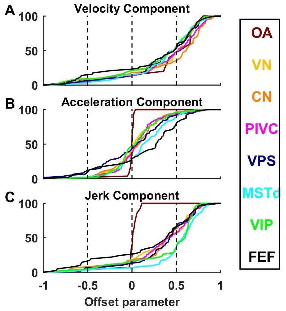
Cumulative distributions of offset parameters for velocity (A), acceleration (B) and jerk (C) components across all brain areas.
Note the larger offset values for velocity and jerk, compared to acceleration.
Figure 10
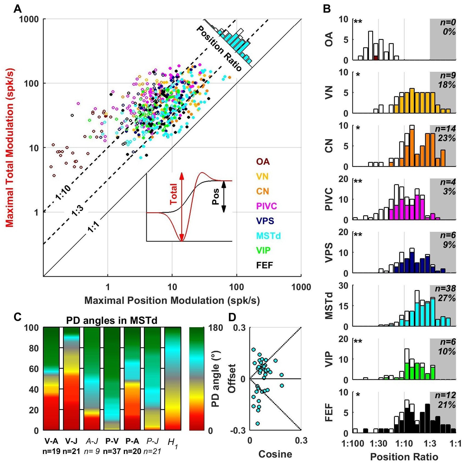
Contribution of position signals to vestibular responses.
(A) Scatter plot of the maximum total peak to peak modulation vs. the maximal position modulation (see inset; computed across all spatial directions for each cell). We define the position ratio as the ratio of these two modulations. The diagonal and the two broken lines represent position ratios of 1:1, 1:3 and 1:10, respectively. (B) Position ratio in all brain areas (the histogram in MSTd is also represented as the marginal cyan distribution in A). The number and percentage of cells with a position ratio higher than 1:3 (grey region) is indicated for each area. All cells that are not significantly tuned to position are represented by open symbols and bars in A and B (and excluded from C,D). (C) Analysis of the angles between the PD of the position (P), velocity (V), acceleration (A) and jerk (J) components (as in Figure 7) for area MSTd. Only cells for which the position ratio is between 1:3 and 1:1 are included (other brain areas are not considered due to the lower numbers of cells). The P and V components have opposite PDs (green) for most MSTd neurons. In contrast, the distribution of P-A angles is symmetric, and similar numbers of cells have aligned and opposite PDs. Accordingly, the distribution of V-A angles is also symmetric. (D) Cosine tuning and offset components of position responses in MSTd (cells with position ratio greater than 1:3). The cells form two groups, one with positive offsets (26/39 cells, median offset = 0.46, [0.41 0.55] CI) corresponding to omnidirectional excitatory responses and another with large negative offsets (13/39 cells, median offset = −0.65, [-0.79–0.49] CI) corresponding to omnidirectional inhibitory responses.
Tables
Table 1
Overview of the data. The table provides a list of the brain regions included in the current analyses, the number (m) of monkeys used in each area (note that neurons were recorded in more than one area in some monkeys), the number (n) of neurons analyzed from each area and references to previous publications where technical details are provided. Neurons were either reported here for the first time (new data) or re-analyzed from previous publications (references in last column).
Area name and abbreviation | m | n | Methodological details and original publication | |
|---|---|---|---|---|
Otolith Afferent fibers, eighth cranial nerve | OA | 2 | 27 | New data/Yu et al. (2015) |
Vestibular Nuclei | VN | 4 | 49 | New data/Liu et al. (2013) |
Rostral medial Cerebellar Nuclei | CN | 5 | 61 | New data/Liu et al. (2013) |
Parietoinsular Vestibular Cortex | PIVC | 2 | 115 | |
Visual Posterior Sylvian area | VPS | 3 | 69 | |
Dorsal Medial Superior Temporal area | MSTd | 3 | 139 | |
Ventral Intraparietal area | VIP | 3 | 62 | |
Frontal Eye Field | FEF | 3 | 57 | |
Total | 19 | 579 | ||
Table 2
Model parameters based on area (median and CI).
OA | VN | CN | PIVC | VPS | MSTd | VIP | FEF | ||
|---|---|---|---|---|---|---|---|---|---|
W0 (spikes/s) | 23 [16-30] | 147 [122-172] | 144 [127-160] | 144 [129-159] | 122 [103-142] | 99 [88-110] | 99 [87-110] | 93 [78-108] | |
Peak-to-trough | 16 [11-21] | 66 [55-78] | 65 [57-73] | 66 [58-73] | 54 [45-63] | 43 [38-48] | 41 [36-47] | 40 [32-47] | |
FR0 (spikes/s) | 74 [61-87] | 41 [34-47] | 49 [43-56] | 19 [15-22] | 12 [9-15] | 18 [16-21] | 11 [10-13] | 15 [11-18] | |
wv | 0.07 [0.05–0.08] | 0.31 [0.28–0.34] | 0.32 [0.30–0.35] | 0.33 [0.31–0.36] | 0.35 [0.32–0.39] | 0.43 [0.41–0.44] | 0.37 [0.34–0.39] | 0.37 [0.33–0.40] | |
wa | 0.60 [0.57–0.63] | 0.40 [0.36–0.45] | 0.37 [0.34–0.41] | 0.41 [0.38–0.43] | 0.38 [0.35–0.42] | 0.30 [0.28–0.33] | 0.38 [0.35–0.41] | 0.37 [0.33–0.40] | |
wj | 0.34 [0.30–0.37] | 0.28 [0.25–0.31] | 0.30 [0.28–0.33] | 0.26 [0.24–0.28] | 0.26 [0.24–0.28] | 0.27 [0.26–0.28] | 0.25 [0.23–0.27] | 0.27 [0.24–0.29] | |
ov | 0.58 [0.32–0.84] | 0.39 [0.26–0.51] | 0.44 [0.32–0.57] | 0.42 [0.34–0.50] | 0.38 [0.28–0.47] | 0.38 [0.32–0.44] | 0.33 [0.22–0.44] | 0.29 [0.16–0.42] | |
oa | 0.00 [-0.01–0.01] | 0.06 [-0.02–0.14] | 0.06 [-0.01–0.14] | 0.07 [0.02–0.12] | 0.02 [-0.07–0.12] | 0.14 [0.09–0.20] | 0.06 [-0.01–0.13] | 0.17 [0.05–0.29] | |
oj | 0.02 [-0.00–0.05] | 0.34 [0.22–0.46] | 0.35 [0.23–0.46] | 0.36 [0.29–0.44] | 0.38 [0.27–0.48] | 0.51 [0.45–0.58] | 0.43 [0.31–0.54] | 0.23 [0.07–0.39] | |
μ0 (s) | 0.06 [0.05–0.07] | 0.04 [0.02–0.07] | 0.04 [0.02–0.07] | 0.04 [0.03–0.05] | 0.05 [0.02–0.07] | 0.14 [0.12–0.16] | 0.07 [0.05–0.10] | 0.06 [0.03–0.09] | |
Best fitting model | V | 0% | 2% | 3% | 4% | 6% | 9% | 6% | 7% |
A | 48% | 2% | 3% | 3% | 1% | 2% | 0% | 0% | |
J | 0% | 0% | 0% | 0% | 0% | 1% | 0% | 0% | |
VA | 0% | 18% | 15% | 17% | 23% | 22% | 19% | 21% | |
VJ | 0% | 4% | 7% | 7% | 4% | 22% | 6% | 9% | |
AJ | 33% | 0% | 5% | 3% | 4% | 0% | 0% | 0% | |
VAJ | 19% | 74% | 67% | 66% | 62% | 44% | 69% | 63% | |
Table 3
p-values of the Kolmogorov-Smirnov tests in Figure 7.
OA | VN | CN | PIVC | VPS | MSTd | VIP | FEF | Sum | |
|---|---|---|---|---|---|---|---|---|---|
V-A PD angles | 0.01 | <10−4 | <10−4 | <10−4 | <10−4 | <10−4 | <10−4 | <10−4 | <10−4 |
V-J PD angles | 0.01 | 0.006 | 0.2 | <10−4 | <10−4 | <10−4 | <10−3 | <10−4 | <10−4 |
A-J PD angles | <10−4 | 0.14 | 0.1 | <10−4 | <10−3 | <10−3 | 0.02 | 0.002 | <10−4 |
Download links
A two-part list of links to download the article, or parts of the article, in various formats.
Downloads (link to download the article as PDF)
Open citations (links to open the citations from this article in various online reference manager services)
Cite this article (links to download the citations from this article in formats compatible with various reference manager tools)
Transformation of spatiotemporal dynamics in the macaque vestibular system from otolith afferents to cortex
eLife 6:e20787.
https://doi.org/10.7554/eLife.20787


