Carbon recovery dynamics following disturbance by selective logging in Amazonian forests
- UMR EcoFoG (Agroparistech, CNRS, Inra, Université des Antilles, Cirad), French Guiana
- UMR EcoFoG (Agroparistech, CNRS, Inra, Université des Antilles, Université de Guyane), French Guiana
- UMR EcoFoG (Agroparistech, Inra, Université des Antilles, Université de Guyane, Cirad), French Guiana
- Cirad, UR Forests and Societies, France
- Embrapa Amazônia Oriental, Brazil
- Wageningen University, Netherlands
- University of Florida, United States
- CarbonForExpert, Switzerland
- University of Oxford, United Kingdom
- Instituto Boliviano de Investigación Forestal, Bolivia
- Embrapa Amazônia Ocidental, Brazil
- Florida International University, United States
- Embrapa Amapa, Brazil
- Instituto de Investigaciones de la Amazonia Peruana, Peru
- Embrapa Acre, Brazil
- University of São Paulo, Brazil
Figures
Figure 1 with 1 supplement
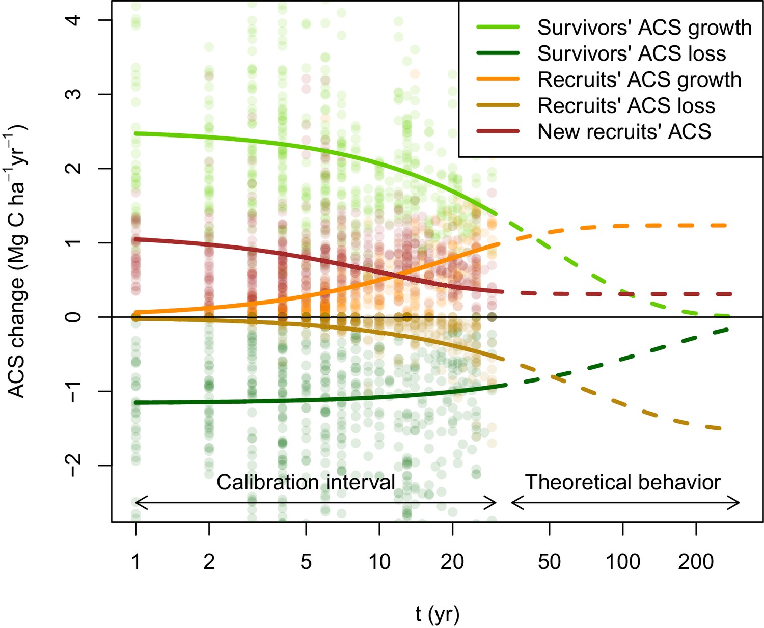
Post-disturbance annual ACS changes of survivors and recruits in 133 Amazonian selectively logged plots.
Data is available between the year of minimum ACS () and 30 years. ACS changes are: recruits’ ACS growth (orange), recruits’ ACS loss (gold), new recruits’ ACS (red), survivors’ ACS growth (light green) and survivors’ ACS loss (dark green). Thick solid lines are the maximum-likelihood predictions (for an average plot, when all covariates are null), and dashed lines are the model theoretical behaviour. New recruits’ ACS, recruits’ ACS growth, and recruits’ ACS loss converge over time to constant values. A dynamic equilibrium is then reached: ACS gain from recruitment and recruits’ growth compensate ACS loss from recruits’ mortality. Survivors’ ACS growth and loss. decline over time and tend to zero when all initial survivors have died.
Figure 1—figure supplement 1
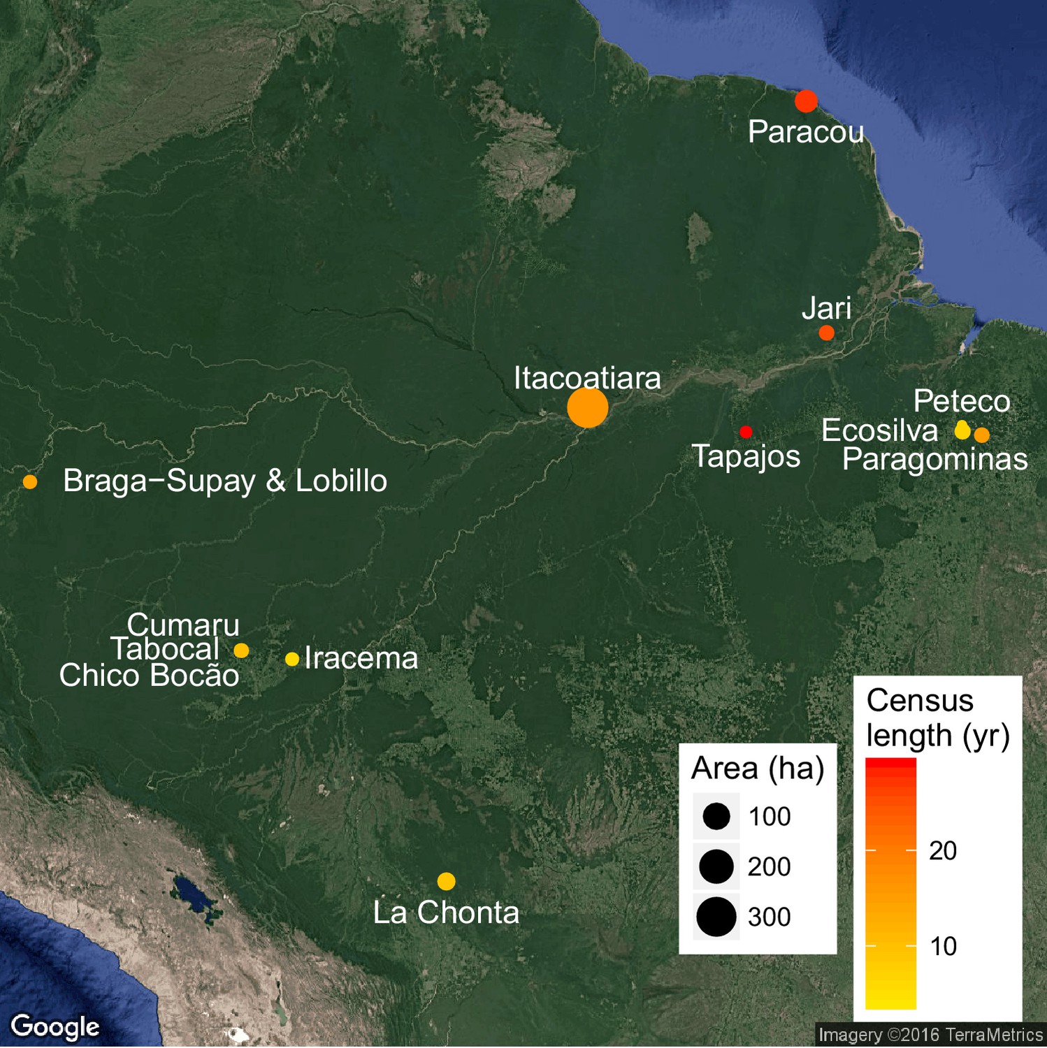
Experimental sites location, each site being composed of permanent forest plots varying in logging intensities, census length (colour) and total area (size).
https://doi.org/10.7554/eLife.21394.004
Figure 2 with 1 supplement
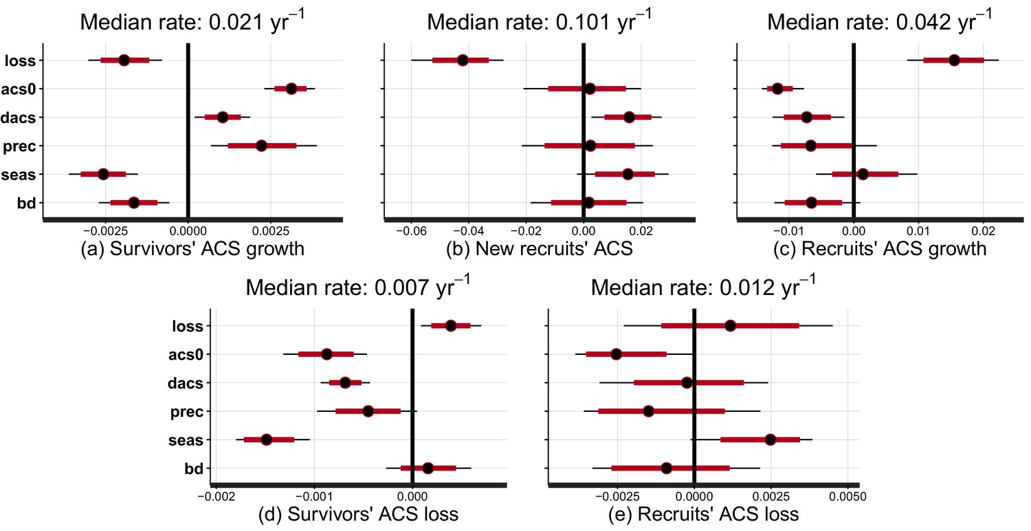
Effect of covariates on the rate at which post-disturbance ACS changes converge to a theoretical steady state (in yr).
Covariates are : disturbance intensity () , i.e. the proportion of initial ACS loss; mean site’s ACS (), and relative forest maturity, i.e. pre-logging plot ACS as a % of (); annual precipitation (); seasonality of precipitation (), soil bulk density (). Covariates are centred and standardized. Red and black levels are 80% and 95% credible intervals, respectively. The median rate is the prediction of the convergence rate for an average plot (when all covariates are set to zero). Negative covariate values indicate slowing and positive values indicate accelerating rates. (a) Survivors’ ACS growth. (b) New recruits’ ACS. (c) Recruits’ ACS growth. (d) Survivors’ ACS loss. (e) Recruits’ ACS loss.
-
Figure 2—source data 1
Parameters posterior distribution.
Columns are the 2.5%, 10%, 50%, 90% and 97.5% quantiles of the posterior distribution of the model parameters (rows).
- https://doi.org/10.7554/eLife.21394.006
Figure 2—figure supplement 1
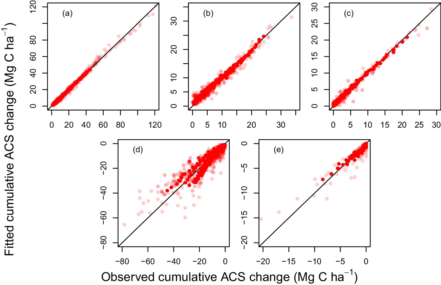
Fitted vs observed values of cumulative ACS changes (Mg C ha).
(a) Survivors’ cumulative ACS growth. (b) New recruits’ cumulative ACS. (c) Recruits’ cumulative ACS growth; (d) Survivors’ cumulative ACS loss; (e) Recruits’ cumulative ACS loss. The closer the dots are to the x=y line, the better the prediction. Dot transparency is proportional to the observation weight: transparent dots are low-weight observations. Because mortality is a stochastic event, ACS loss has poorer predictions than ACS gain which is a more continuous process.
Figure 3
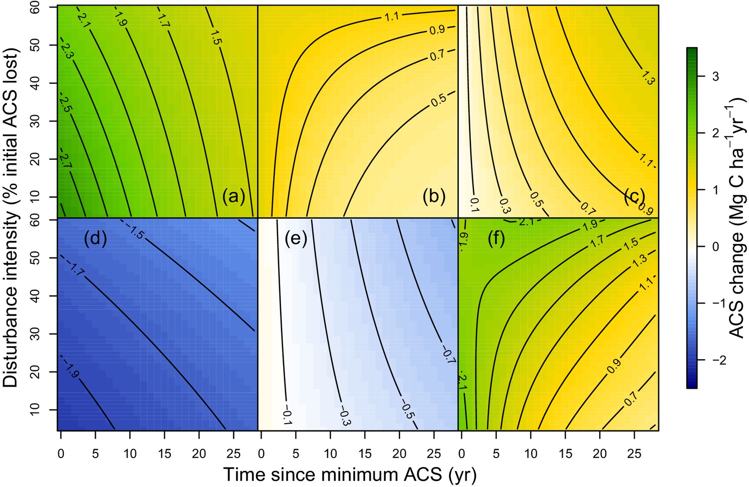
Predicted effect of disturbance intensity on ACS changes along time in an Amazonian-average plot.
(a) Survivors’ ACS growth. (b) New recruits’ ACS. (c) Recruits’ ACS growth. (d) Survivors’ ACS loss. (e) Recruits’ ACS loss. (f) Net ACS change. The net ACS change is the sum of all five ACS changes. ACS changes were calculated with all parameters set to their maximum-likelihood value and covariates (except standardized disturbance intensity ) set to 0. Time since minimum ACS varies from 0 to 30 year (i.e. the calibration interval) and disturbance intensity ranges between 5% and 60% of initial ACS loss.
Figure 4
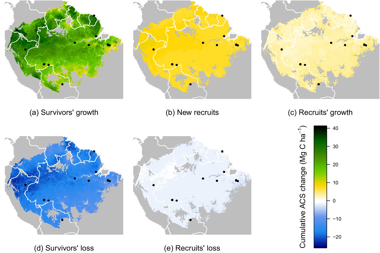
Predicted cumulative ACS changes (Mg C ha) over the first 10 year after losing 40% of ACS.
Extrapolation was based on global rasters: topsoil bulk density from the Harmonized global soil database (Nachtergaele et al., 2008), Worldclim precipitation data (Hijmans et al., 2005) and biomass stocks from Avitabile et al. map (Avitabile et al., 2016). Cumulative ACS changes are obtained by integrating annual ACS changes through time. We here show the median of each pixel. Top graphs are ACS gain and bottom graphs are ACS loss. (a) ACS gain from survivors’ growth. (b) ACS gain from new recruits. (c) ACS gain from recruits’ growth. (d) ACS loss from survivors’ mortality. (e) ACS loss from recruits’ mortality. Black dots are the location of our experimental sites. Survivors’ ACS changes (a and d) show strong regional variations unlike to recruits’ ACS changes (b,c and e).
Figure 5
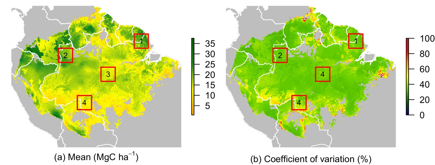
Predicted net ACS recovery over the first 10 year after losing 40% of pre-logging ACS.
(a) median predictions. (b) coefficient of variation (per pixel). Four areas were arbitrarily chosen to illustrate four different geographical behaviours: (1) the Guiana Shield and (2) northwestern Amazonia are two areas with high ACS recovery; the Guiana Shield has higher initial ACS and slower ACS dynamics whereas northwestern Amazonia has lower initial ACS and faster ACS dynamics. (3) central Amazonia has intermediate ACS recovery. (4) southern Amazonia has low ACS recovery.
Figure 6

Predicted contribution of annual ACS changes in ACS recovery in four regions of Amazonia (Figure 5).
The white line is the net annual ACS recovery, i.e. the sum of all annual ACS changes. Survivors’ (green) and recruits’ (orange) contribution are positive for ACS gains (survivors’ ACS growth, new recruits’ ACS and recruits’ ACS growth) and negative for survivors’ and recruits’ ACS loss. Areas with higher levels of transparency and dotted lines are out of the calibration period (0–30 year). In the Guiana Shield and in nothwestern Amazonia, high levels of net ACS recovery are explained by large ACS gain from survivors’ growth. Extrapolation was based on global rasters: topsoil bulk density from the Harmonized global soil database (Nachtergaele et al., 2008), precipitation data from Worldclim (Hijmans et al., 2005) and biomass stocks from Avitabile et al. (Avitabile et al., 2016) map.
Appendix 1—figure 1
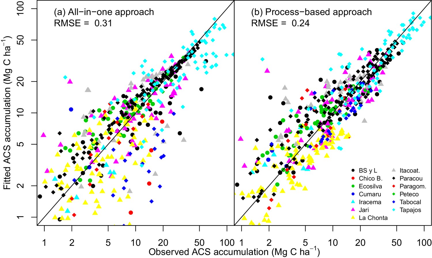
Observed vs fitted values of net ACS accumulation (MgC ha).
(a) Fitted values from the all-in-one model. (b) Fitted values from the process-based model (right). Net ACS accumulation is the sum of cumulative ACS changes (gain and loss). Each combination of a colour and shape is specific to a site. The closer the dots are to the x=y line, the better the prediction.
Appendix 1—figure 2
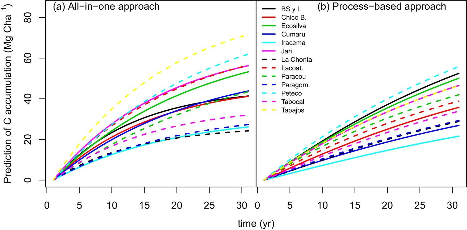
Predicted trajectories of net ACS accumulation (MgC ha) per site with (a) the all-in-one model and (b) the process-based model.
https://doi.org/10.7554/eLife.21394.014
Author response image 1

Time to recover 50% of initial ACS per region and disturbance intensity.
https://doi.org/10.7554/eLife.21394.015
Author response image 2
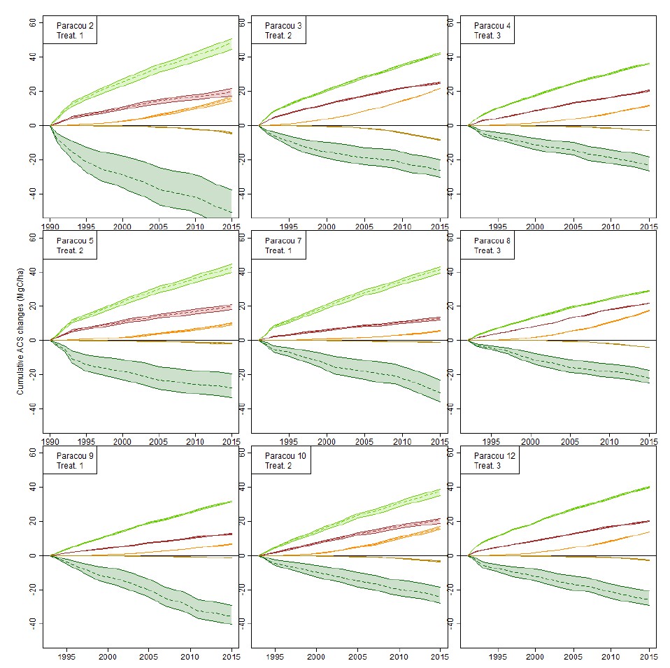
Effect of botanical indetermination on cumulative ACS changes in the 9 Paracou forest plots.
Wood density of all undetermined trees is set to 0.4 (lower bound), 0.9 (higher bound), or the plot average wood density (dashed lines): the latter is the method used in the study. Cumulative ACS changes are then calculated. Cumulative ACS changes (MgC/ha) are: survivors’ ACS growth (light green), survivors’ ACS loss (dark green), new recruits’ ACS (red), recruits’ growth (orange), recruits’ ACS loss (ocher).
Tables
Table 1
List of priors used to infer ACS changes in a Bayesian framework. Models are : () survivors’ ACS growth, () survivors’ ACS loss, () new recruits’ ACS, () recruits’ ACS growth, () recruits’ ACS loss. is the parameter relative to the covariate (logging intensity).
| Model | Parameter | Prior | Justification |
|---|---|---|---|
| On average 100 survivors/ha storing 0.25 to 2.5 MgC each | |||
| yr | |||
| yr | |||
| Range of observed values in TmFO control plots | |||
| yr | |||
| Range of observed values in Amazonia (Johnson et al., 2016) | |||
| yr | |||
| yr | |||
| All models M† | Avoid multicollinearity problems | ||
| All models M† | Avoid multicollinearity problems |
-
∗ is the time when the ACS change has reached 95% of its asymptotic value.
-
†M is one of the five models: either , , , , .
Download links
A two-part list of links to download the article, or parts of the article, in various formats.
Downloads (link to download the article as PDF)
Open citations (links to open the citations from this article in various online reference manager services)
Cite this article (links to download the citations from this article in formats compatible with various reference manager tools)
Carbon recovery dynamics following disturbance by selective logging in Amazonian forests
eLife 5:e21394.
https://doi.org/10.7554/eLife.21394


