Humans treat unreliable filled-in percepts as more real than veridical ones
- Institute of Cognitive Science, University of Osnabrück, Germany
- University of Hamburg, Germany
- University Medical Center Hamburg-Eppendorf, Germany
Figures
Figure 1 with 1 supplement
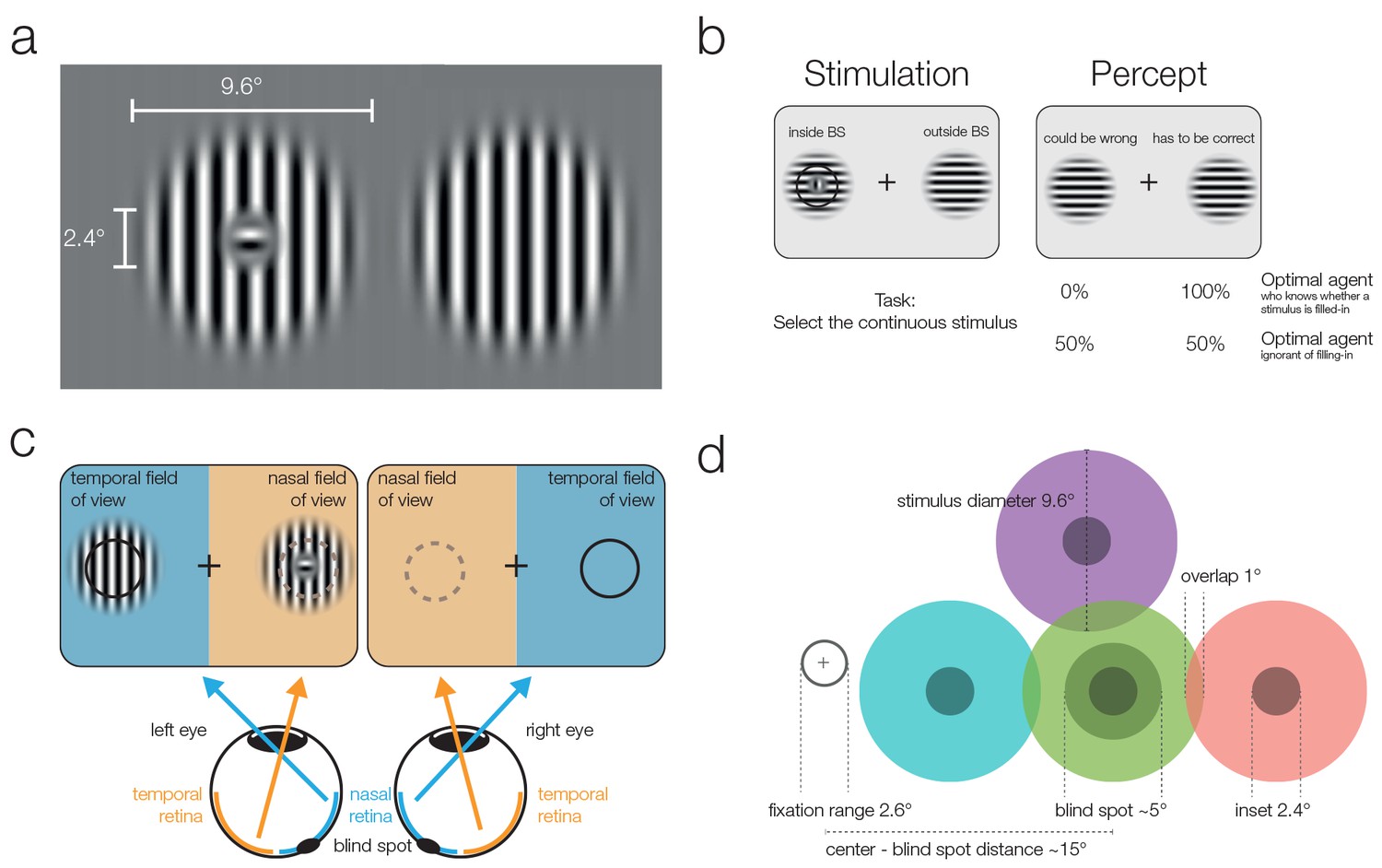
Stimuli and stimulation.
(a) Striped stimuli used in the study. The inset was set to ~50% of the average blind spot size. The global orientation of both stimuli was the same, but in different trials it could be either vertical (as shown here) or horizontal (not shown). (b) Each stimulus was displayed individually either (partially) inside or (completely) outside the blind spot. This example presents an inset stimulus inside the subject’s left blind spot. However, due to filling-in, it is perceived as continuous (right column). The task required subjects to select the continuous stimulus, and it was designed to differentiate between two mutually exclusive predictions: First, subjects cannot differentiate between the two different types of stimuli and thus answer randomly. Alternatively, subjects have implicit or explicit knowledge about the difference between inferred (filled-in) and veridical contents and consequently select the stimulus outside the blind spot in ambiguous trials. (c) Two stimuli were displayed using shutter glasses. Each stimulus was presented to one eye only, and it is possible that both are presented to the same eye (as in the example depicted here). That is, the left stimulus could be shown either in the temporal field of view (nasal retina) of the left eye (as in the plot) or in the nasal field of view (temporal retina) of the right eye (not shown). In this case, the trial was unambiguous: The stimulus with an inset was presented outside the blind spot and could be veridically observed, therefore, the correct answer was to select the left stimulus. (d) The locations of stimulus presentation in the five experiments. All stimuli were presented relative to the blind spot location of each subject. All five experiments included the blind spot location (green). In the second and fifth experiment, effects at the blind spot were contrasted with a location above it (purple). In the third experiment, the contrasts were in positions located to the left or the right of the blind spot. Note that both stimuli were always presented at symmetrical positions in a given trial, the position of the stimuli differed only across trials.
Figure 1—figure supplement 1
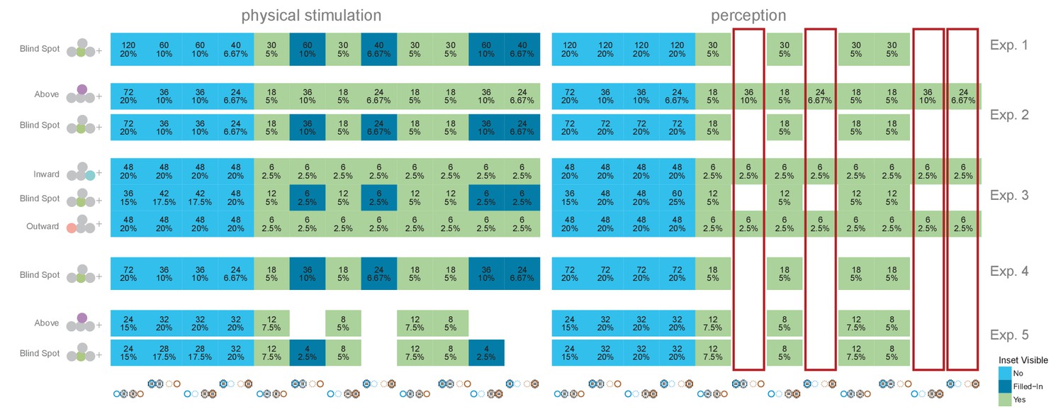
Trial balancing of all experiments.
Each row is one condition in one experiment (depicted in the left most column). The graph is split in a physical stimulation (what is shown, left) and a perception column (what do subjects perceive due to fill-in in the blind spot, right). The dark-blue fields depict trials where an inset stimulus (dark-blue) was shown but partially inside the blind spot. On the right side (perception) we added these trials to the respective continuous (blue) cases. We mark with red the columns that indicate trials where an inset was shown in the temporal field. Note that perceptually these trials only exist in the locations above/inward/outward the blind spot, but are impossible inside the blind spot (due to fill-in). Because the resulting statistical distribution might influence decisions by the subjects (see results of experiment 5, probability matching), experiment 5 was a repetition of experiment 2 without these trials.
Figure 2
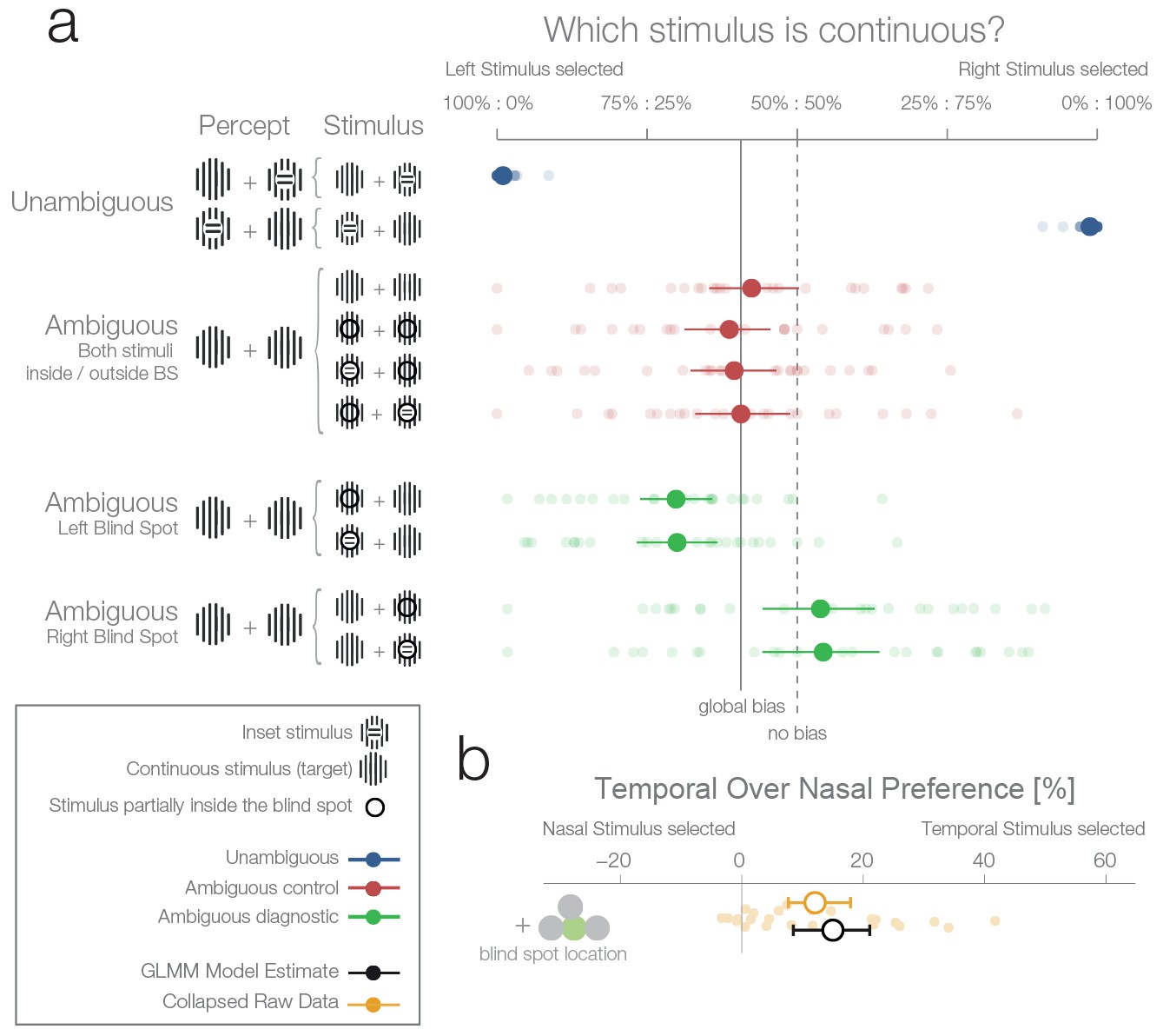
First experiment.
(a) The left column shows schematics of the actual stimulation and the associated percepts for the corresponding data presented in the right panel. A dark-lined circle, where present, indicates that the stimulus was presented in the blind spot and, consequently, an inset stimulus within was perceived as a continuous stimulus due to filling-in. The plot to the right shows each subject’s (n = 24) average response and the group average (95% bootstrapped confidence intervals, used only for visualization). The results from unambiguous trials (blue) show that subjects were almost perfect in their selection of the continuous stimulus when an inset was visible. For the first type of ambiguous control trials (red), both stimuli were presented either outside or inside the blind spot. Here, only a global bias toward the left stimulus can be observed (solid line, the mean across all observed conditions in red). Note that the performance when presenting an inset in the blind spot was identical to the one of presenting a continuous stimulus in the blind spot. The ambiguous diagnostic conditions (green) show the, unexpected, bias toward the blind spot (for either side). (b) Statistical differences were evaluated by fitting a Bayesian generalized mixed linear model. In the model, the left and right ambiguous diagnostic conditions were combined in a single estimate of the bias for nasal or temporal stimuli (outside or inside the blind spot respectively). The plot shows the average effect of each subject (small yellow dots), the bootstrapped summary statistics of the data (yellow errorbar), and the posterior 95% credibility interval model estimate (black errorbar).
Figure 3

Location control experiments.
Two control experiments were designed to test whether the observed bias for the blind spot could be explained by a general bias for stimuli presented in the temporal visual field. (a) Results of experiment 2. In a given trial, stimuli were presented either at the locations corresponding to the blind spot or at locations above it. Results are presented as in Figure 2b, with the addition of within-subject differences between blind spot and control locations (in purple). (b) Results of experiment 3. In a given trial, stimuli were presented at the locations corresponding to the blind spot or at locations to inward (toward the fixation cross) or outward (away from the fixation cross) to it. Note that the blind spot effect is replicated in both experiments. In addition, both blind spot effects are larger than in any control location.
Figure 4 with 1 supplement
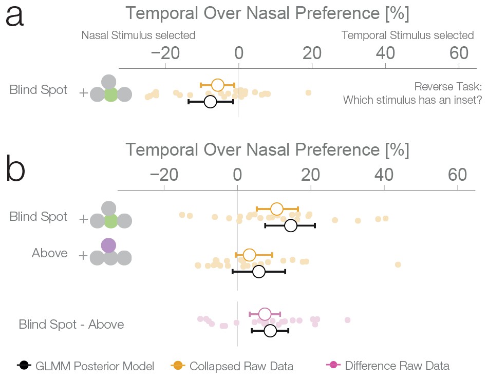
Task instruction control and probability matching control.
(a) Results of experiment 4. This control was the same as experiment 1, except that subjects have to choose the stimulus with an inset (instead of the continuous one). (b) Results of experiment 5. This control was similar to experiment 2, except that no inset stimulus was ever experienced in the control location above in the temporal visual field.
Figure 4—figure supplement 1
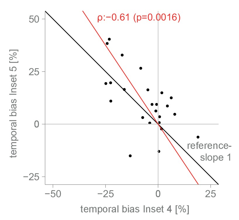
Correlation between experiment 4 and 5.
Global-bias subtracted blind spot effect for each subject in experiment 4 and 5. Subjects showed a negative bias towards the nasal stimulus outside the blind spot in experiment 4 (the task-switch experiment) and a positive bias towards the temporal stimulus inside the blind spot in experiment 5. The reference line has a slope of 1. The red line is the first principle component (representing total least squares). The Pearson correlation coefficient is 0.61 (p=0.0016).
Figure 5
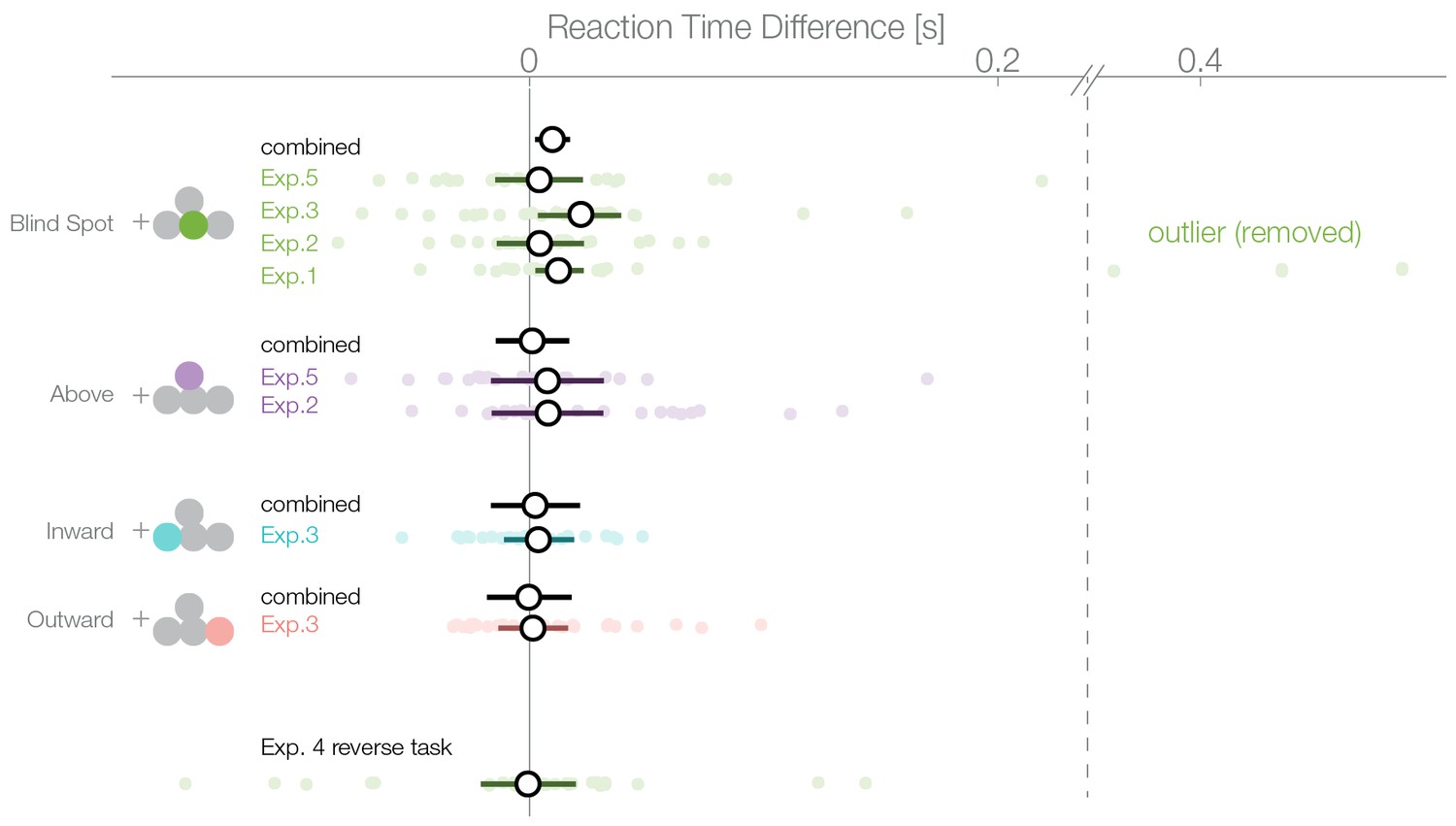
Reaction times.
Reaction times of trials where the nasal stimulus was chosen minus the reaction times of trials where the temporal stimulus was chosen. Single subject estimates and 95% CI posterior effect estimates are shown. The black (combined) estimate results from a model fit of all data combined, the individual confidence intervals represent the experiment-wise model fits. We observe a reaction time effect only inside the blind spot.
Figure 6 with 2 supplements
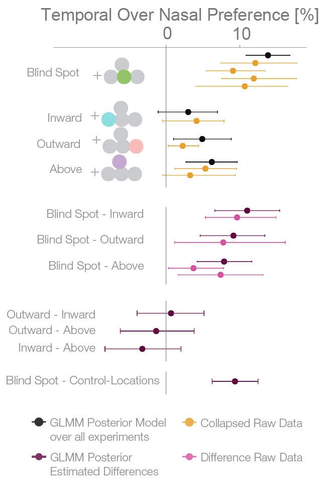
Summary and overview of blind spot effects.
Posterior GLMM-effect estimates of all data combined (black) except experiment 4 (inversed task). We also show for each experiment the 95% CI of bootstrapped means summary statistics of the data (yellow). Next, we show difference values between the blind spot and all other control locations (model dark, raw data pink). As discussed in the text, the control locations outward, inward and above do not differ (fourth last to second last row), and thus we compare the blind spot effect to all locations combined (last row).
Figure 6—figure supplement 1
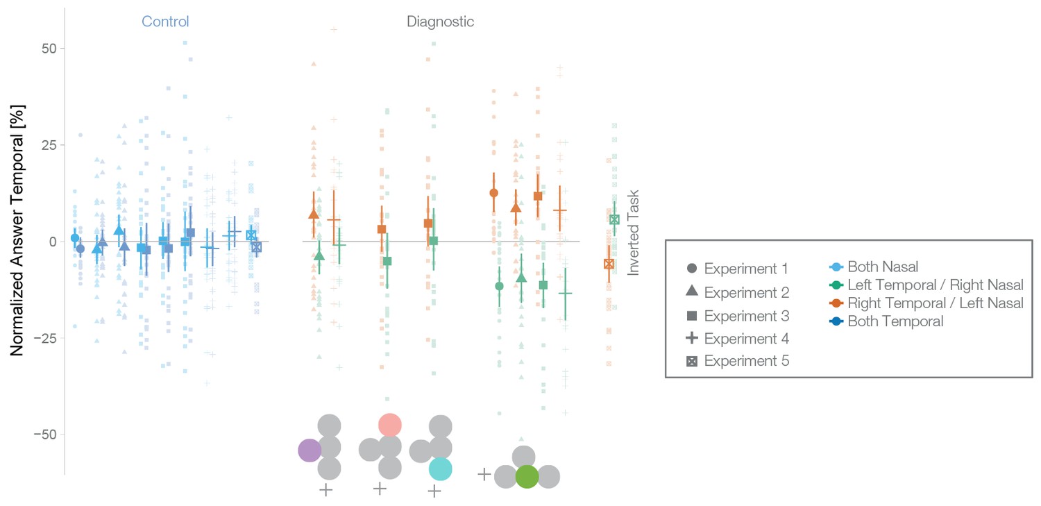
Normalized data with control locations for all experiments.
Fraction of choosing the right stimulus dependent on location (indicated by icon) and experiment (Exp. 1: n = 24, Exp. 2: n = 27, Exp. 3: n = 24, Exp. 4: n = 25, Exp. 5: n = 24). For plotting purposes, we preprocessed the data of each subject by subtracting their respective global bias. Each gray dot depicts one subject. The error bars depict mean, and 95% bootstrapped CI. A bias for the blind spot was visible in the form of ‘left’ responses when the left stimulus was presented in the temporal visual field of the left eye (green, nasal/blind spot retina of the left eye) and of more ‘right’ responses when the right stimulus was presented in the temporal visual field of the right eye (green, nasal/blind spot of the right eye) in all experiments. A bias was visible in the other tested locations, but it was much smaller. Control conditions show that there was no bias if the stimuli were shown either both inside the temporal fields (dark blue) or both inside the nasal fields (light blue).
Figure 6—figure supplement 2
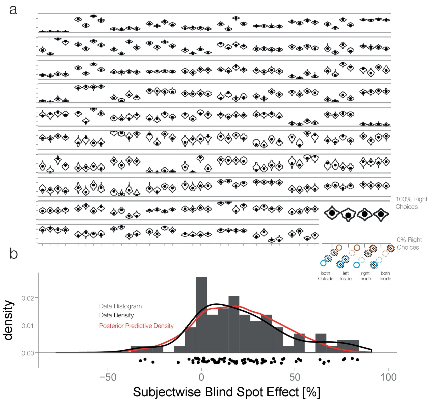
Posterior predictive checks.
(a) First level posterior predictive check: We simulated 100 new datasets from the posterior with the subject-wise posterior effect estimates. The observed values (black dots) are adequately captured for all subjects depicted here. (b) Second level posterior predictive check: Here we estimated datasets with new subjects randomly sampled from the multi-variate mixed-effects population distribution. We calculated the subject-wise blind spot effect, collapsed over both blind spots. The posterior predictive estimates are shown in red. They match the empirical distribution of blind spot effects (black line, histogram and scatter plot below) closely. We conclude that our model is adequate to capture the patterns of interest in our study.
Additional files
-
Supplementary file 1
Overview of the results of all experiments individually and the combined estimates.
Empty cells indicate that the condition was not measured in this study.
- https://doi.org/10.7554/eLife.21761.013
Download links
A two-part list of links to download the article, or parts of the article, in various formats.
Downloads (link to download the article as PDF)
Open citations (links to open the citations from this article in various online reference manager services)
Cite this article (links to download the citations from this article in formats compatible with various reference manager tools)
Humans treat unreliable filled-in percepts as more real than veridical ones
eLife 6:e21761.
https://doi.org/10.7554/eLife.21761


