When complex neuronal structures may not matter
- Brandeis University, United States
- Harvard Medical School, United States
Figures
Figure 1
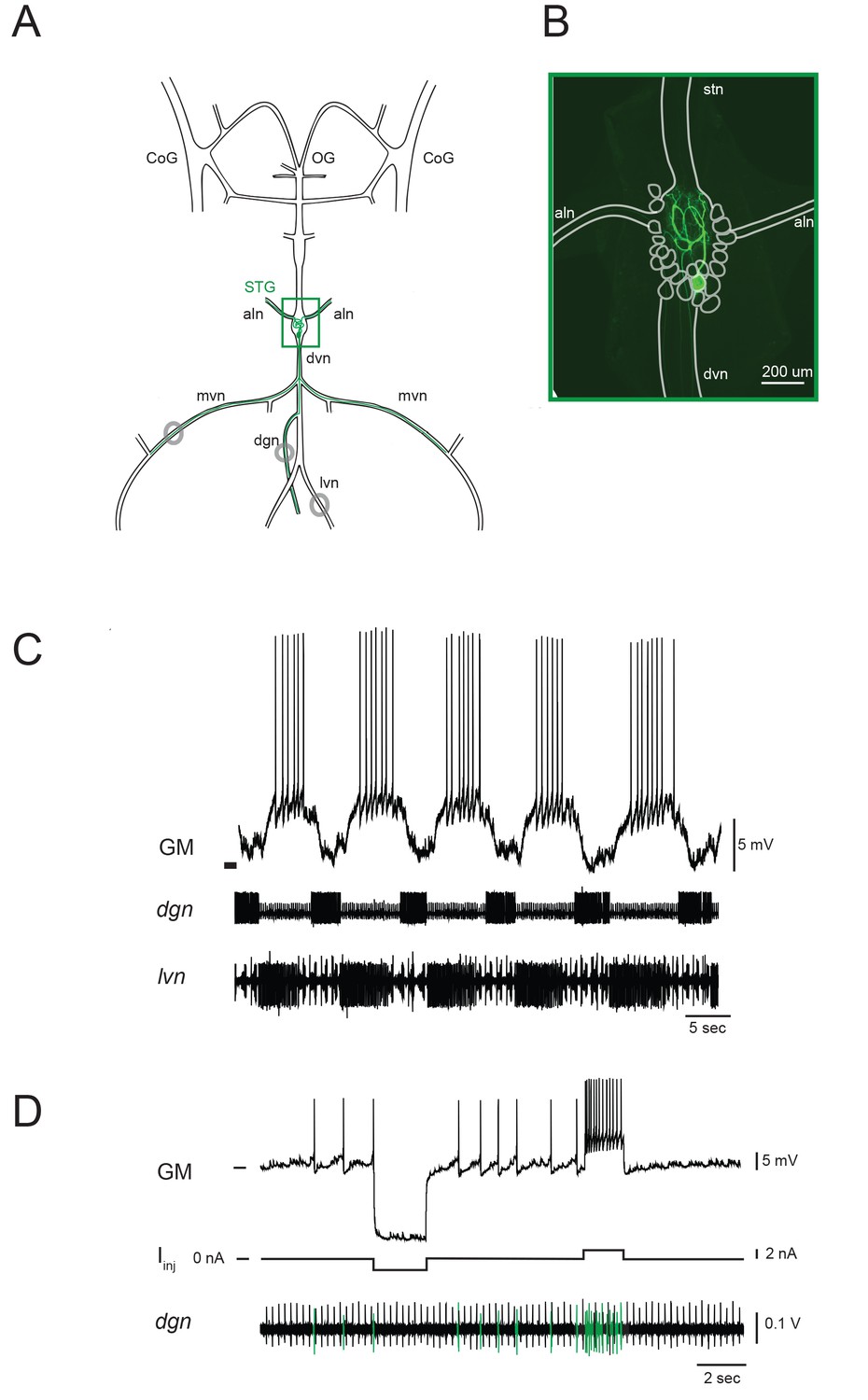
The stomatogastric nervous system (STNS) and identification of gastric mill (GM) neurons.
(A) Schematic of an in vitro, isolated STNS with descending inputs intact (from bilateral commissural ganglia (CoGs) and esophogeal ganglion (OG)). The stomatogastric ganglion (STG; green box) contains identifiable motor neurons that project their axons onto specific muscle groups via the medial ventral nerve (mvn), anterior lateral nerves (aln), dorsal ventricular nerve (dvn) and lateral ventricular nerve (lvn), and dorsal gastric nerve (dgn). An example of the axonal projection path of a GM neuron is shown in green. Extracellular nerve recordings (locations indicated with gray circles) are utilized for physiological identification of GM neurons (as in D). (B) Example of an alexa488 dye-fill (green) of a GM neuron, with the STG, nerve projections, and other neurons outlined in white. (C) The GM neuron participates in a slow, episodic gastric mill rhythm that is highly conserved across animals. Top: an intracellular recording of GM with simultaneous extracellular nerve recordings of the dgn and lvn show concurrent, single-neuron and circuit-level activities. (D) GM neurons are identified physiologically by matching intracellular spike activity with extracellular nerve spike units in the dgn, which contains GM axonal projections (shown in green on dgn). Hyperpolarizing and depolarizing current pulses (Iinj) make this identification unambiguous. These identifications are verified with microscopy and identification of axons projecting bilaterally into the alns, as in B. In C and D, horizontal bars indicate an intracellular voltage of −50 mV.
Figure 2
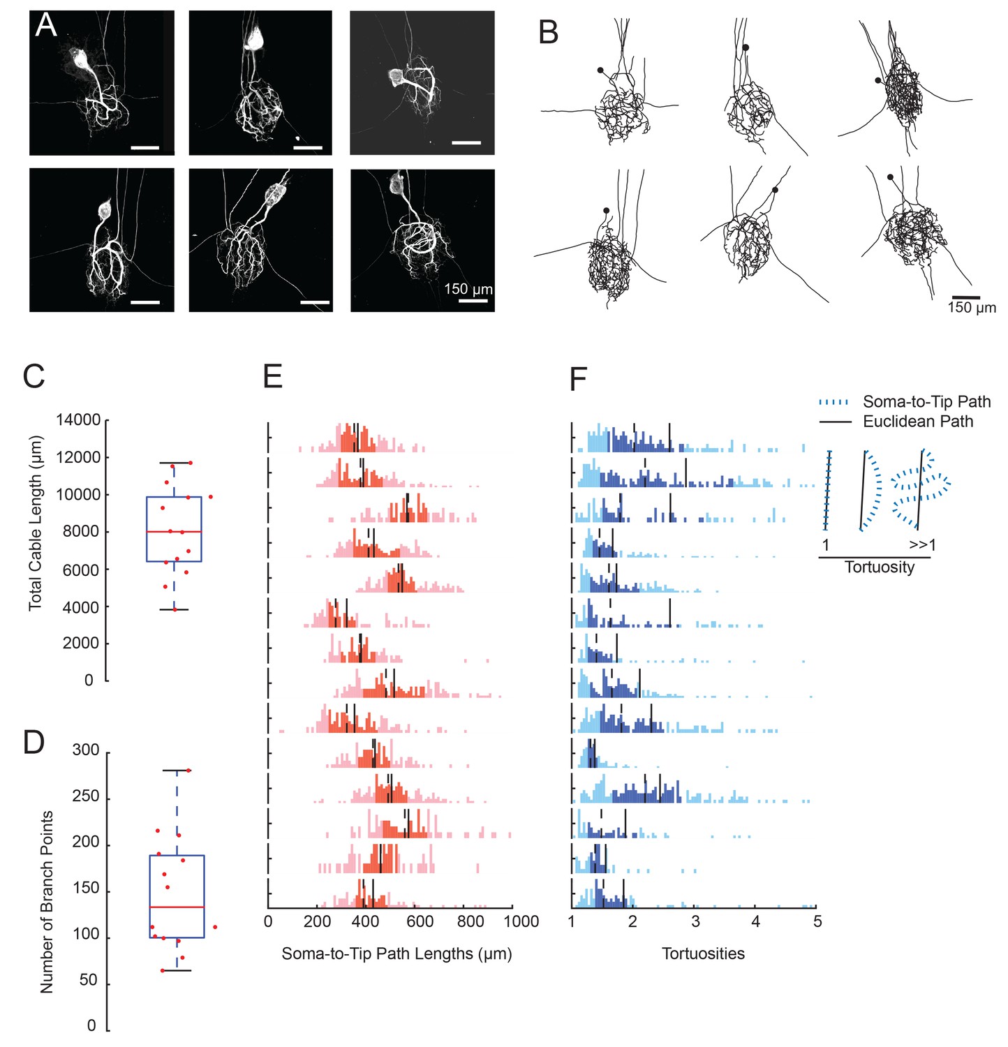
GM neurons exhibit expansive and complex morphologies.
(A) Maximum z-projections of 3-dimensional confocal image stacks capturing Lucifer yellow dye-fills of six GM neurons (taken at 20x magnification). (B) Skeletal reconstructions of the six neurons shown in A, generated by manual tracing in KNOSSOS software and used for quantitative morphological analyses shown in C-–F. All scale bars in A and B are 150 µm. (C) Boxplot of total cable lengths (excluding axonal projections; Mean + SD = 8112.6 + 2453.6 µm). (D) Boxplot of the total number of branch points (excluding axonal branch points; mean + sd = 148 + 63 branch points). For C and D, red line indicates the median, the blue box spans the 25th and 75th percentiles, and the whiskers span the range of data points not considered to be outliers. (E) Histograms show the distributions of paths from soma to terminating neurite for individual GM neurons (from top to bottom). (F) Histograms showing the tortuosities for soma-to-tip paths for individual GM neurons (from top to bottom). Tortuosity was calculated as the ratio of measured soma-to-tip path length (as in E) over the Euclidean distance from soma to tip. On right, diagram indicates the interpretation of tortuosity for a given path (blue) relative to the Euclidean distance (black). For E and F, the darker shaded region spans the 25th and 75th percentiles, solid lines indicate the mean, and dashed lines indicate the median. The y-axes are scaled to the maximum number of paths among bins within each neuron. Note the leftward bias in the tortuosity distributions (F). For C–F, metrics were calculated for N = 14 GM neurons in 14 different animals.
Figure 3
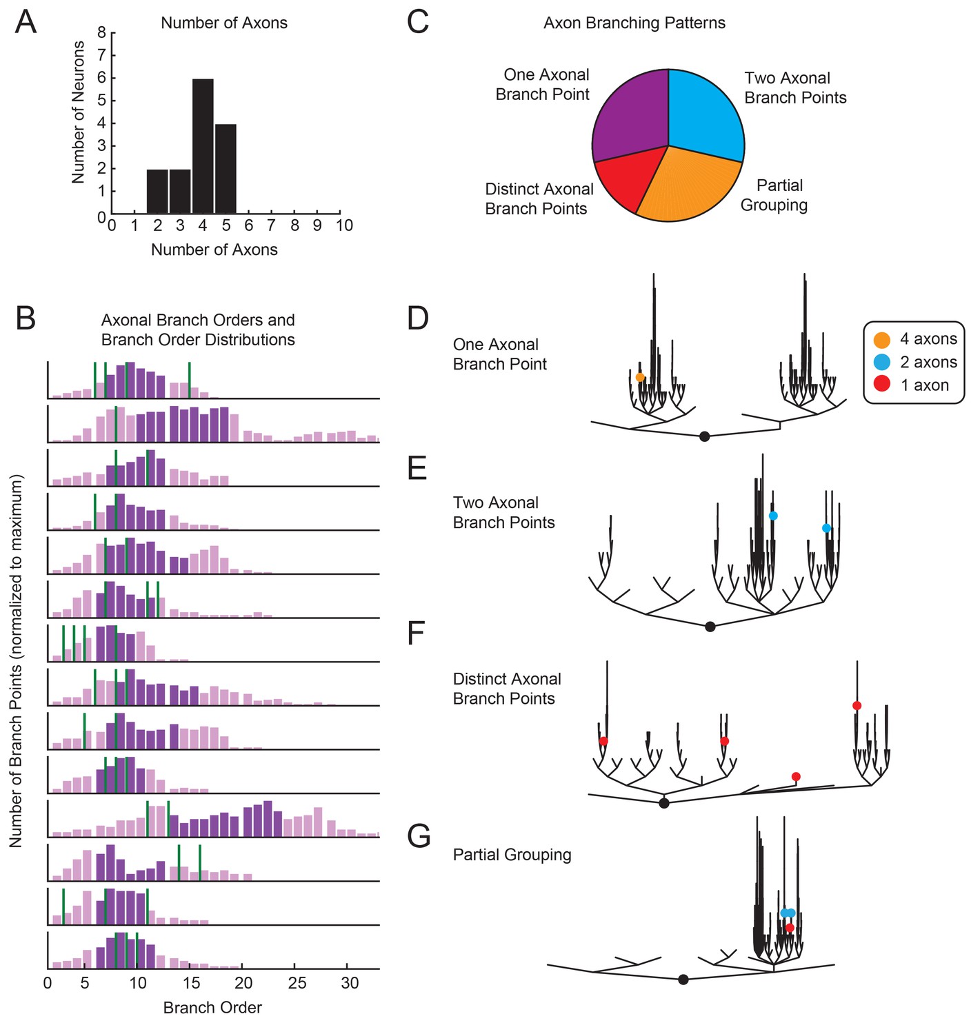
Variable axon location and branching patterns in GM neurons.
(A) Histogram shows the number of distinguishable axonal projections for 14 GM neurons. (B) Histograms show the distribution of branch orders across 14 GM neurons. Axonal branch point orders are indicated with green lines. Dark purple shading indicates the range between the 25th and 75th percentiles. For easy comparison across neurons, histograms were plotted with 100 bins and y axes were normalized to the maximum number of branch points given the 100 bins. (C) Pie chart summarizes axonal branching patterns across 14 GM neurons. (D–G) Examples of the different axonal branching pattern possibilities in C are illustrated with dendrograms of four GM neurons from the tested population. Axonal branch points are indicated with colored circles indicating the number of axons projected from that branch point: orange = 4 axons, blue = 2 axons, red = 1 axon.
Figure 4 with 1 supplement
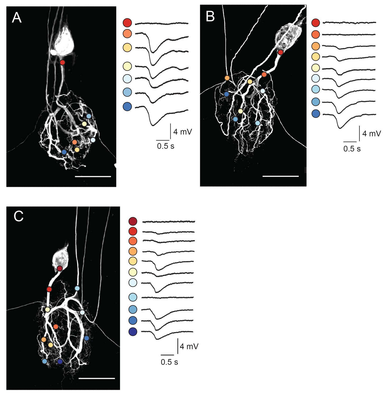
Focal glutamate responses across GM neuronal structures.
(A–C) show maximum z-projections of confocal stacks of neuronal dye-fills with photo-uncaging sites indicated with colored circles. In each case, raw traces are shown on the right for maximal inhibitory glutamate responses evoked with 1 ms pulses at 30 mW UV laser intensity while. holding the membrane potential at −40 mV using two-electrode current clamp at the somatic recording site. Note the variability in response amplitude across different photo-uncaging sites within each neuron. Image scale bars are 150 µm.
Figure 4—figure supplement 1
Focal glutamate photo-uncaging resolution and response desensitization.
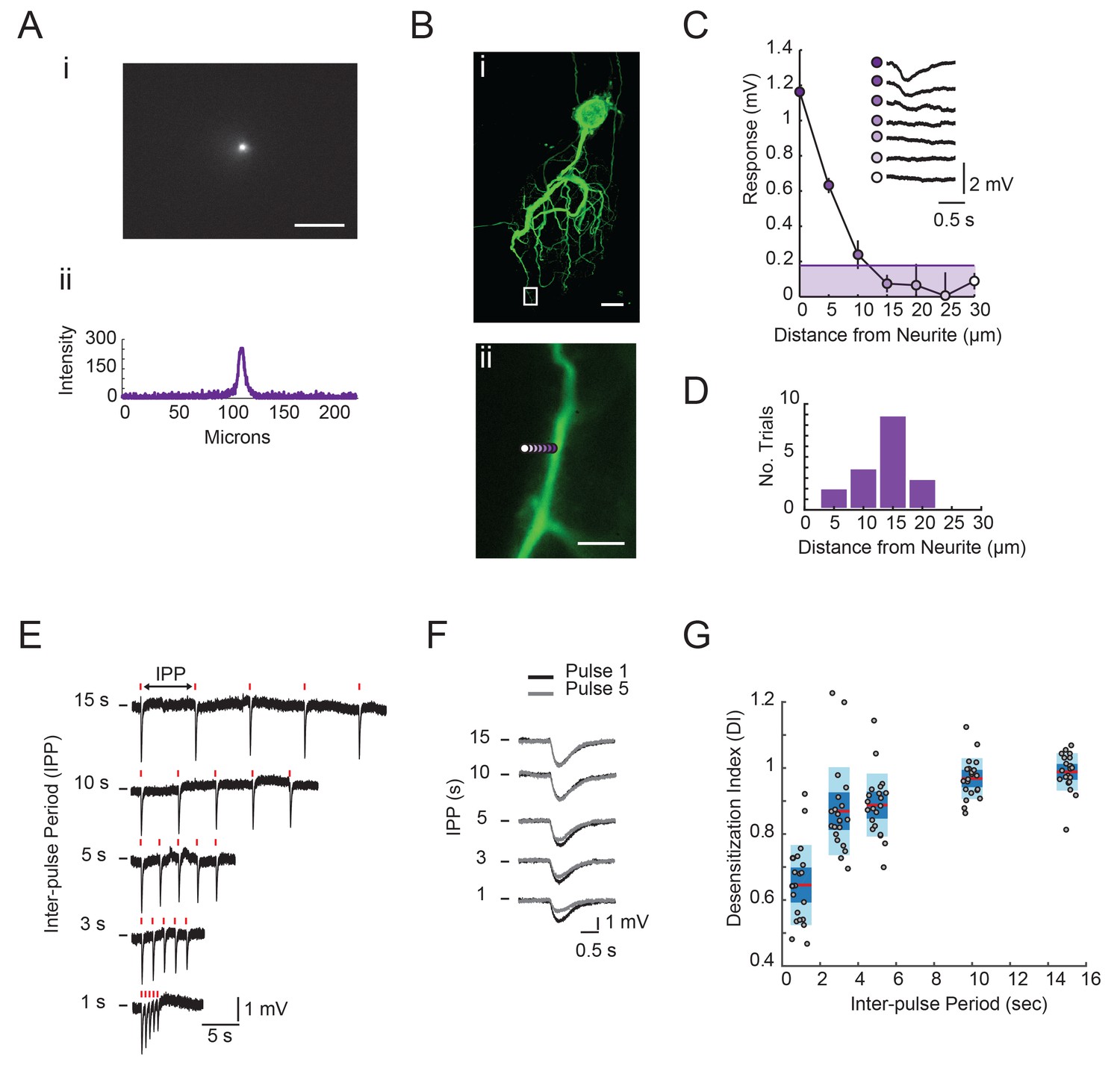
(A) Image of UV spot emission in fluorescein solution (top). Line intensity. profile (bottom) shows a saturated spot diameter of ~15 microns. (B) (i) Maximum projection of a confocal image stack of Lucifer yellow dye-filled GM neuron (20x magnification). (ii) Boxed region from (i) with UV spot photo-uncaging positions indicated with purple, with opacity that decreases with distance. (C) Plot of response amplitude (inverted) as a function of distance form neurite. (as indicated in Bii). Inset shows raw responses at each position. Line and shaded area denote 15% maximum response amplitude cut-off used to generate histogram in D. (D) Histogram showing the distance from neurite at which the response amplitude was <15% of the maximum response at a given position. Y-axis is the number of trials or positions (n = 18) sampled across 11 different STG neurons. Scale bars in A and B are 50 microns. (E) Raw traces of focal glutamate responses evoked at one position on a single GM neuron with varying inter-pulse periods (IPPs). 1 ms, 30 mW stimuli are times are indicated with red lines above traces. (F) Overlaid responses from first (black) and fifth (gray) pulses in stimulus trains shown in E. In E and F, horizontal bars indicate starting membrane potential of −40 mV. Desensitization indices (DI) were calculated by dividing the peak amplitude of the response to the fifth pulse in the stimulus train (gray) by the peak amplitude of the response to the first pulse in the stimulus train (black). A DI = 1 indicates no desensitization. (G) DI as a function of inter-pulse period across 22 photo-uncaging sites in five different neurons. Red lines indicate the median. DI values, dark blue shaded boxes indicate the standard deviations, and light blue boxes indicate the 95% confidence intervals.
Figure 5 with 1 supplement
Response amplitudes as a function of various cable properties.
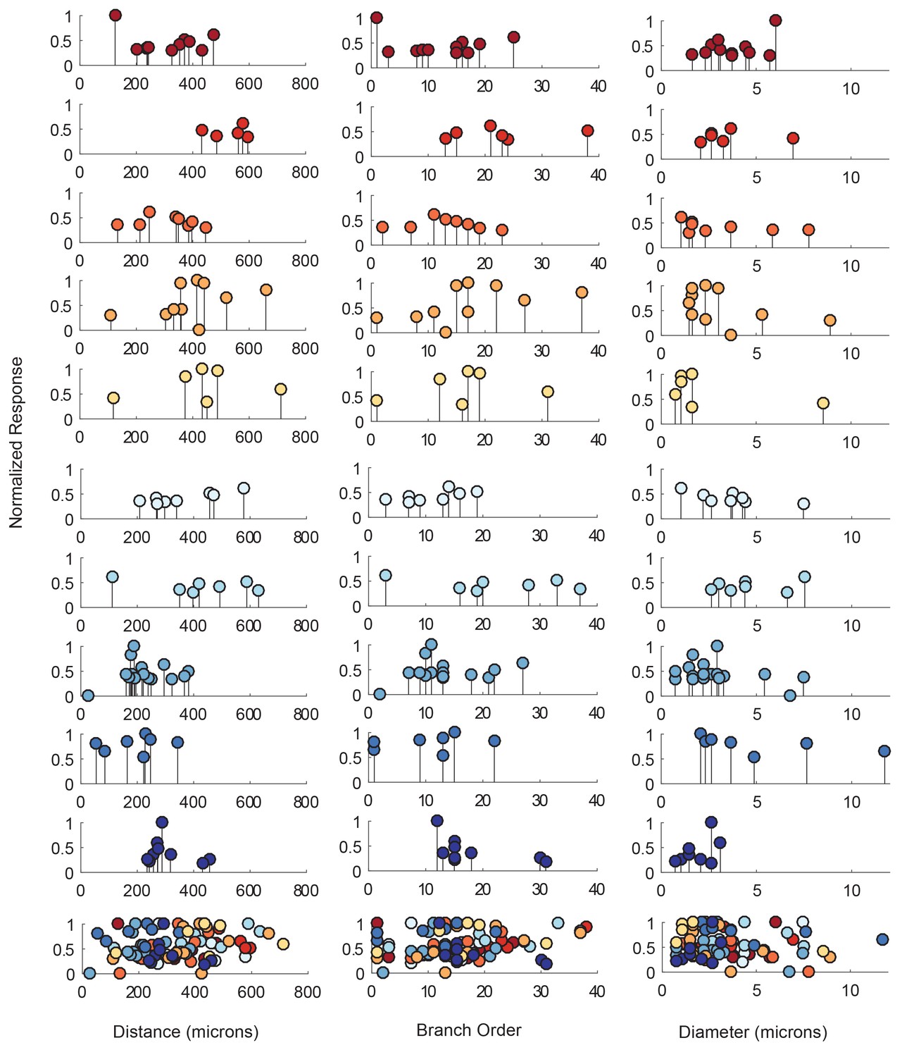
Each lolliplot shows the normalized maximal response amplitudes for photo-uncaging sites that vary in distance from the soma, branch order, and neurite diameter. Each color is indicative of focal responses from a single neuron (N = 10). Focal glutamate responses were evoked at a depolarized membrane potential (−40 or −50, constant within each neuron), in two-electrode current clamp at the soma. Scatter plots at the bottom show these same data from all 10 neurons on the same axes. To allow comparison across neurons, voltage responses. were normalized to the maximum voltage response within each preparation. Distance and branch order measurements were generated from skeletal reconstructions. Diameter measurements were measured manually from neuronal dye-fill confocal stacks. Results from linear regression analyses of the above data are shown in the Figure 5—figure supplement 1 and in Table 1.
Figure 5—figure supplement 1
Response amplitudes as a function of various cable properties with raw response amplitudes and linear fits.
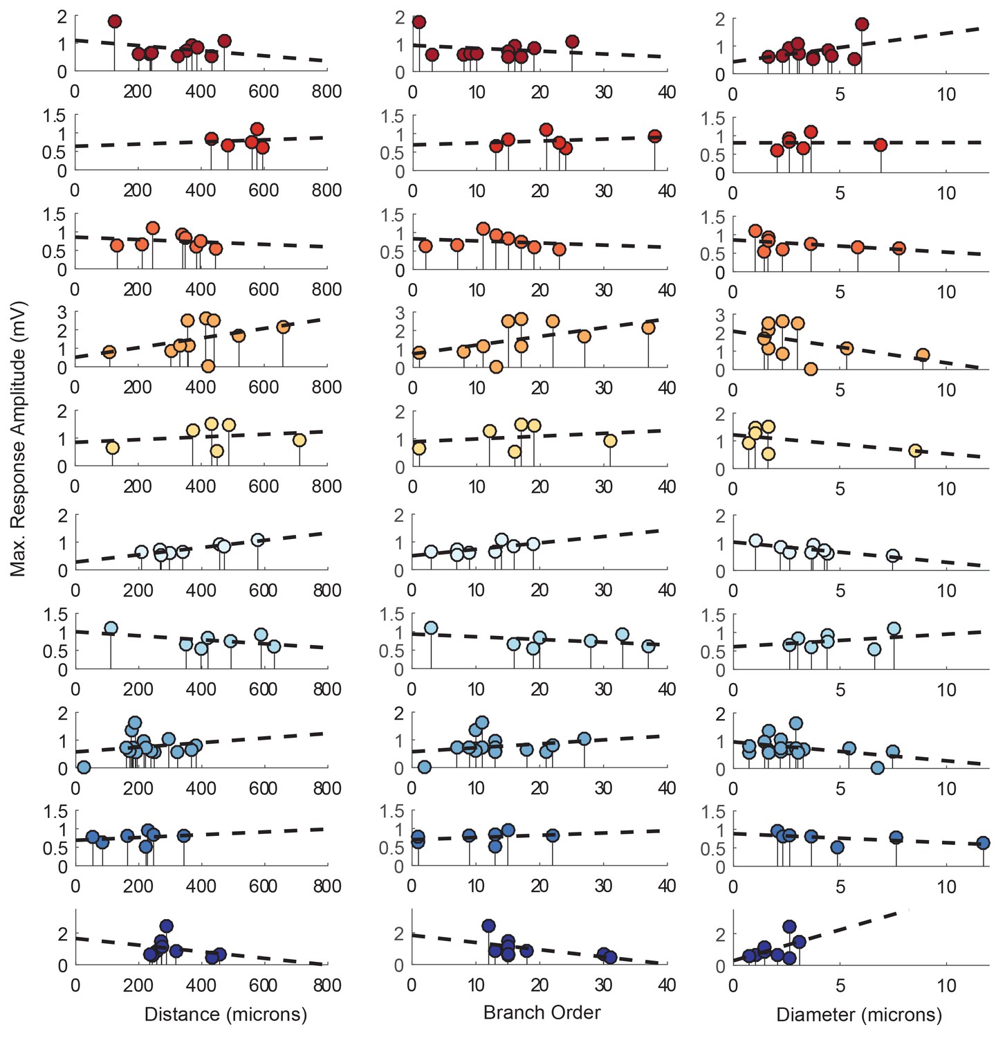
Each lolliplot shows the maximal response amplitudes in mV for photo-uncaging sites that vary in distance from the soma, branch order, and neurite diameter. Each color is indicative of focal responses from a single neuron (N = 10). Focal glutamate responses were evoked at a depolarized membrane potential (−40 or −50, constant within each neuron), in two-electrode current clamp at the soma. Distance and branch order measurements were generated from skeletal reconstructions. Diameter measurements were measured manually from neuronal dye-fill confocal stacks. Linear regression analyses were completed for each of the plotted data and the fits (however poor) are plotted on same axes (dashed black lines). Statistics from these analyses were insignificant across all 10 preparations and shown in Table 1.
Figure 6 with 1 supplement

Passive cable simulations show that apparent Erev measurements are independent of maximal conductance (gmax) and dependent on the distance between activation and recording sites.
(A) An inhibitory current (actual Erev = −70 mV, τ = 3 ms) was activated 200 µm from the recording site (at 0 µm). (B) Voltage events as measured at 0 µm. The membrane potential at the recording site was manipulated with current injections between −8 and + 2 nA. Colors correspond to responses evoked at 200 µm with different gmax values (as indicated). (C) (i) Response amplitude (deltaV) plotted as a function of membrane potential (Vm) as measured at 0 µm. Apparent Erevs were identified for each gmax by calculating the x- intercept of linear fits to these curves (R > 0.9 and p<0.01 in all cases). The inset shows a magnification along the x-axis and illustrates that all curves share the same x-intercept, regardless of. gmax value. (ii) Apparent Erev plotted as a function of gmax values. (D) To determine the dependence of apparent Erev as a function of activation site distance from recording site, inhibitory currents (Erev = −70 mV, τ = 3 ms, gmax = 5 nS) were evoked at 0, 200, 400, 600, 800,. and 1000 µm from the recording site. (E) Voltage events as measured at 0 µm. The membrane. potential at the recording site was manipulated with current injections between −8 and + 2 nA. Colors correspond to responses evoked at different activation sites (as indicated in D). (F) (i) Response amplitude (deltaV) plotted as a function of membrane potential (Vm) as measured at 0 µm. Apparent Erevs were identified for each activation site distance by calculating the x-intercept of linear fits to these curves (R > 0.9 and p<0.01 in all cases). The inset shows a magnification along the x-axis and illustrates the hyperpolarizing shift in apparent Erev as activation site distance increases. This is explicitly plotted in (ii). The cable model used to generate all of these data had a passive conductance of 20 nS·cm−2 and axial resistance of 30 Ω·cm (see Materials and methods).
Figure 6—figure supplement 1
The apparent Erev remains independent of gmax, regardless of the activation site’s distance from the recording site.
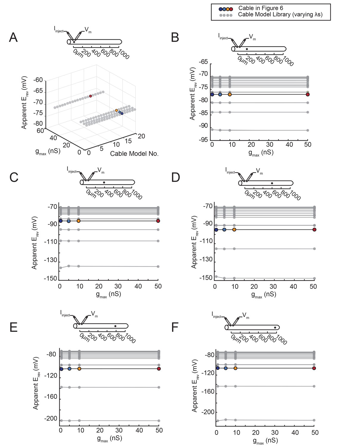
An inhibitory current (actual Erev = −70 mV) was evoked at varying distances from the recording site 0 µm. (A–F) All plots show apparent Erevs as a function of gmax (1, 5, 10, 50 nS) for all 20 passive cable models (in gray), varying in their membrane and axial resistances (see Materials and methods). The data points in color denote the same cable model presented in Figure 6, with a passive conductance of 20 nS·cm−2 and axial resistance of 30 Ω·cm (as indicated in key at top). The cable diagrams above each plot indicate the recording and activation sites. (A) When measured at the site of activation (0 µm), the apparent Erev is equivalent to the actual Erev, regardless of gmax or passive properties. B–F When the inhibitory current is activated at 200 (B), 400 (C), 600 (D), 800 (E), or 1000 (F) µm away, the apparent Erev measured at 0 µm is independent of gmax, but does vary with passive properties.
Figure 7
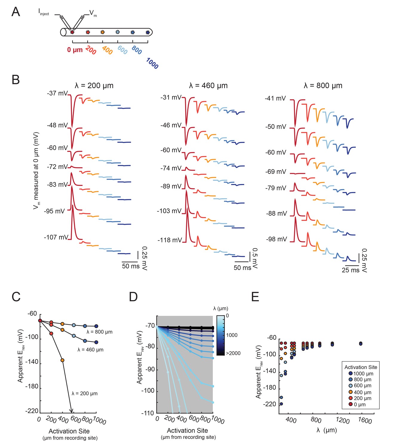
The shift in apparent Erev with activation site distance is contingent upon the electrotonic length constant, λ.
(A) For each of the 20 cable models, with varying passive properties and, consequently, λ values (see Materials and methods), an inhibitory current (actual Erev = −70 mV) was evoked at varying distances from the recording site 0 µm. (B) Voltage events as measured at 0 µm for cables with λ = 200, 460, and 800 µm. The membrane potential at the recording site (Vm) was manipulated with current injections between −8 and + 2 nA. Colors correspond to responses evoked at different activation sites (as indicated in A and Figure 6D). With increasing activation site distance, the voltage deflections flip sign at increasingly hyperpolarized Vms at the recording site. This hyperpolarizing shift is more drastic in the cable with the lowest λ. (C) Plot of the apparent Erev (measured at 0 µm) as a function of activation site distance, in the three cables shown in B. The colors are indicative of the activation site distance, as in the traces in B. (D) Plot of apparent Erev (measured at 0 µm) as a function of activation site distance for all 20 cable models. The blue colorbar indicates relative λ values, ranging between 200 µm and 5 mm. (E) Plot of apparent Erev (measured at 0 µm) as a function of λ, as measured in cables with λs between 300 and 1600 µm. As λ increases, apparent Erevs of responses evoked at different activation site distances converge toward the actual Erev.
Figure 8 with 1 supplement
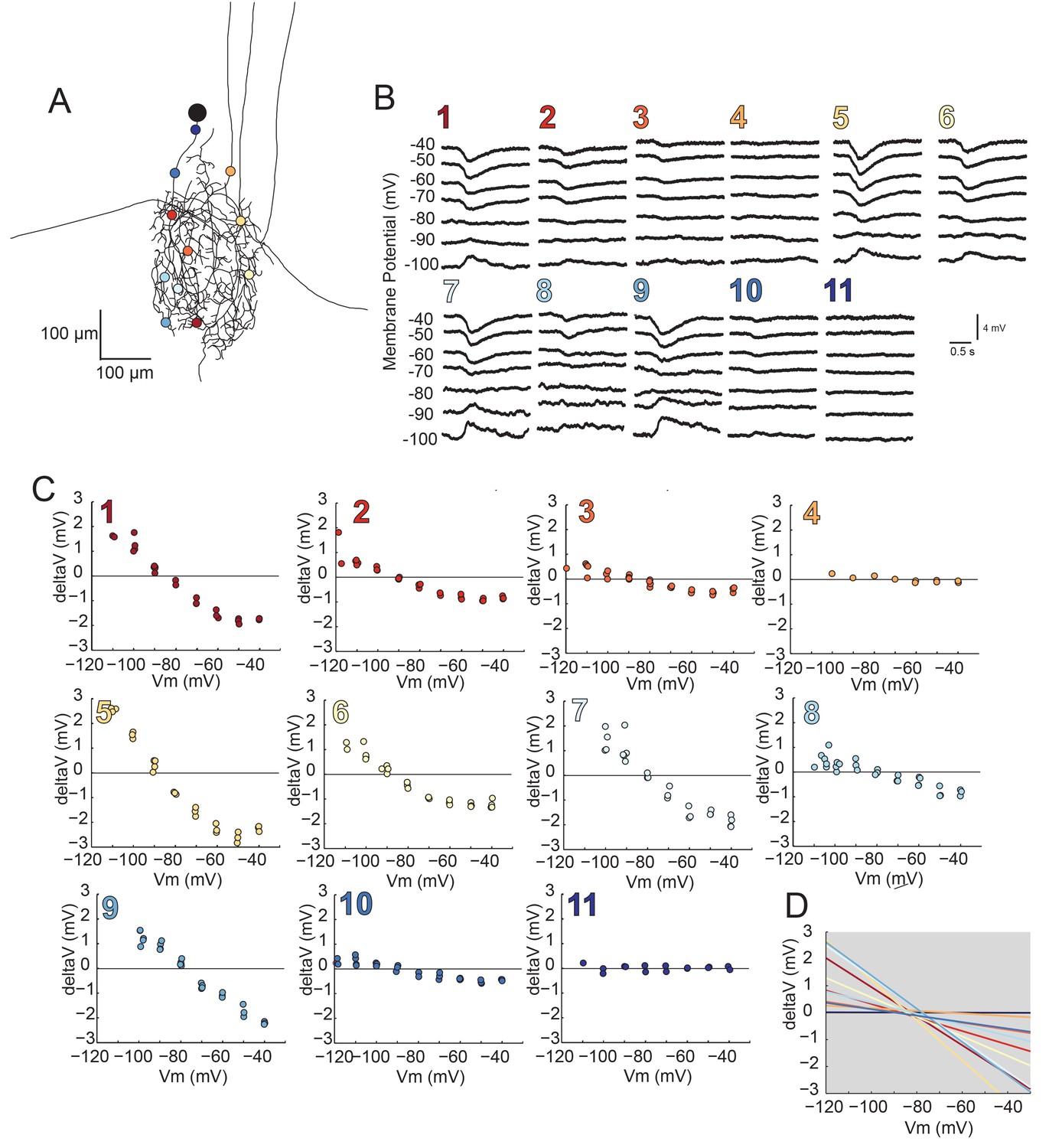
Reversal potentials are nearly invariant across individual neuronal structure.
(A) Photo-uncaging sites are indicated as unique colors on the skeletal reconstruction of one GM neuron. (B) Raw voltage traces show focal glutamate responses as measured at the soma in two-electrode current clamp when evoked at positions indicated in A. (C) Plots of response peak amplitude (deltaV) as a function of membrane potential at soma (Vm) for each photo-uncaging site. (D) Linear functions for each position generated by linear regression analyses of data shown in C. Note that the x-intercepts (apparent Erevs) are highly invariant across photo-uncaging sites. The mean apparent Erev + SD = −84.6 + 4.3 mV and coefficient of variation (CV) is 0.05 in this neuron.
Figure 8—figure supplement 1
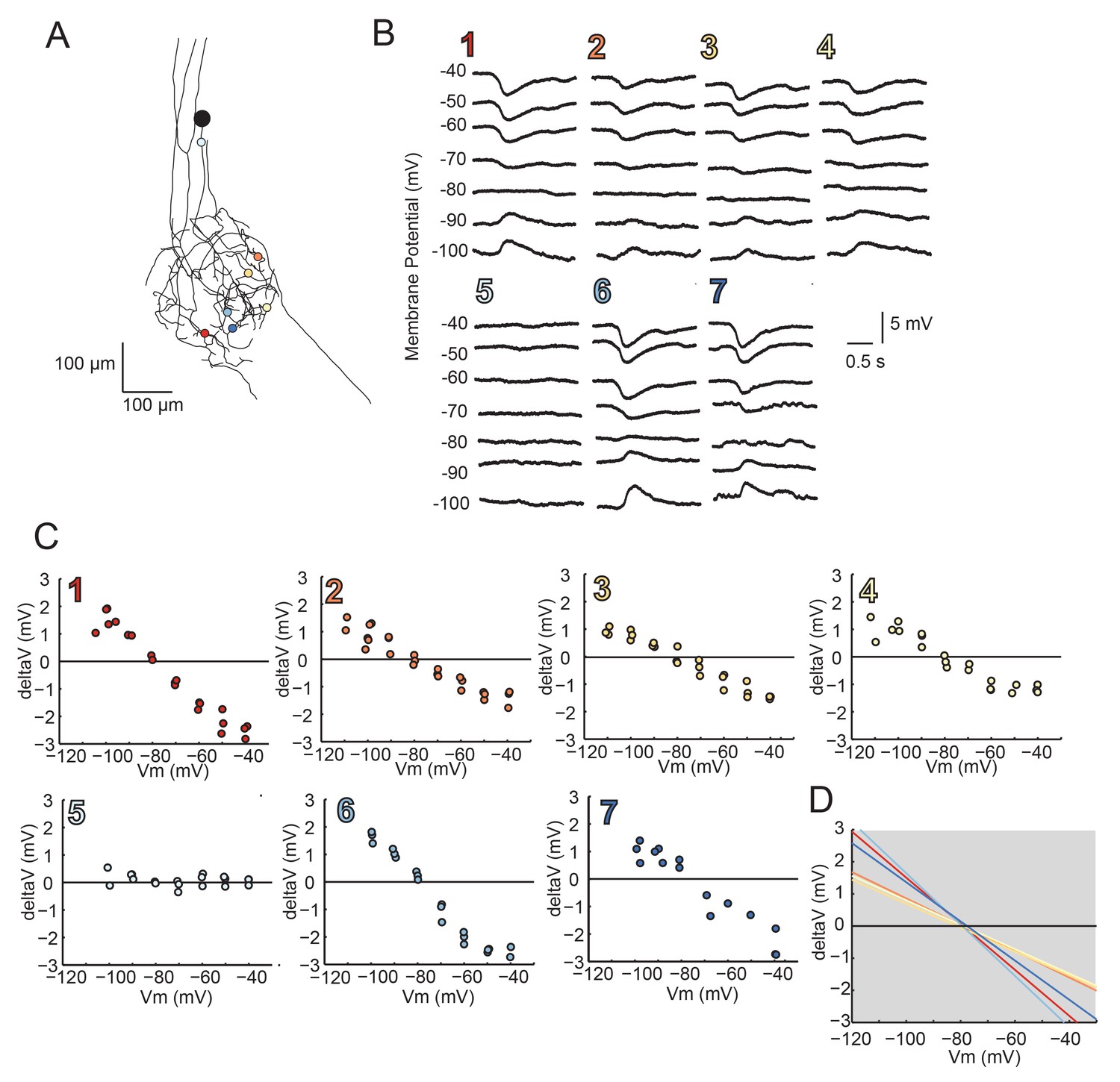
Reversal Potentials are nearly invariant across individual neuronal structure, a second example.
(A.) Photo-uncaging sites are indicated as unique colors on the skeletal reconstruction of one GM neuron. (B) Raw voltage traces show focal glutamate responses as measured at the soma in two-electrode current clamp when evoked at positions indicated in A. (C) Plots of response peak amplitude (deltaV) as a function of membrane potential at soma (Vm) for each photo-uncaging site. (D) Linear functions for each position generated by linear regression analyses of data shown in C. Note that the x-intercepts (apparent Erevs) are highly invariant across photo-uncaging sites. The mean apparent Erev + SD = −79.2 + 1.2 mV and coefficient of variation (CV) is 0.02 in this neuron.
Figure 9 with 1 supplement

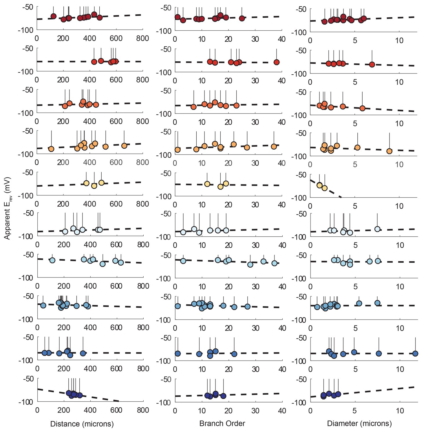
Reversal potentials as a function of various cable properties.
Each lolliplot shows the glutamate response apparent reversal potentials (Erevs) for photo-uncaging sites as function of their distance from the soma, branch order, and neurite diameter. Each color and lolliplot is indicative of the set of reversal potentials across sites within a single neuron (N = 10). Focal glutamate responses were evoked at varying membrane potentials (between −120 and −40 mV) with two-electrode current clamp at the soma. Apparent Erevs for each photo-uncaging site were determined as in Figure 6. Distance and branch order measurements were generated from skeletal reconstructions. Diameter measurements were generated by manual measurement of neuronal dye-fill confocal stacks.
Figure 9—figure supplement 1
Reversal potentials as a function of various cable properties with linear fits.
Each lolliplot shows the glutamate response apparent reversal potentials (Erevs) for photo-uncaging sites as function of their distance from the soma, branch order, and neurite diameter. Each color and lolliplot is indicative of the set of reversal potentials across sites within a single neuron (N = 10). Focal glutamate responses were evoked at varying membrane potential (between −120 and −40 mV) with two-electrode current clamp at the soma. Apparent Erevs for each photo-uncaging site were determined as in Figure 6. Distance and branch. order measurements were generated from skeletal reconstructions. Diameter measurements were generated by manual measurement of neuronal dye-fill confocal stacks. The above plots were fit were linear regression analyses. The resulting linear functions are plotted on the same axes (dashed black lines). Across all 10 preparations and cable properties, slopes were nearly. zero. Statistics for the linear regression analyses are shown in Table 2.
Figure 10
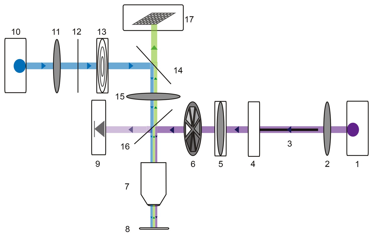
Microscope schematic showing laser (purple), fluorescence excitation (blue), and fluorescence emission (green) paths.
A 1 Watt 355 nm laser (1) is focused by a plano-convex lens (2) and coupled to a 50-micron fiber optic cable (3) situated on an x-y translating fiber adaptor (4). The UV beam is collimated with a plano-convex lens situated in a z-translator (5). The beam intensity can be manually adjusted with a neutral density filter wheel (6) and passes through a 40x UV water immersion objective (7) onto the STNS preparation (8). The UV beam intensity is measured in real-time with a calibrated photo-diode (9) measuring a signal proportional to the power administered to the preparation. A 470 nm blue LED (10) is collimated by a plano-convex lens (11) and passes through a 466/40 nm band-pass filter (12) and field diaphragm (13). This light is re-directed by a 495 nm dichroic beamsplitter (14) and passes through a tube lens (15) and 405 nm low-pass dichroic beamsplitter (16). This is directed through the same 40x objective (7) and excites the alexa488 dye-filled preparation. This fluorescence passes through the 405 nm low-pass dichroic beamsplitter (16), tube lens (15), and 495 nm dichroic beamsplitter (14) and is subsequently captured by the CCD array of a firewire monochrome camera (Scientifica).
Figure 11
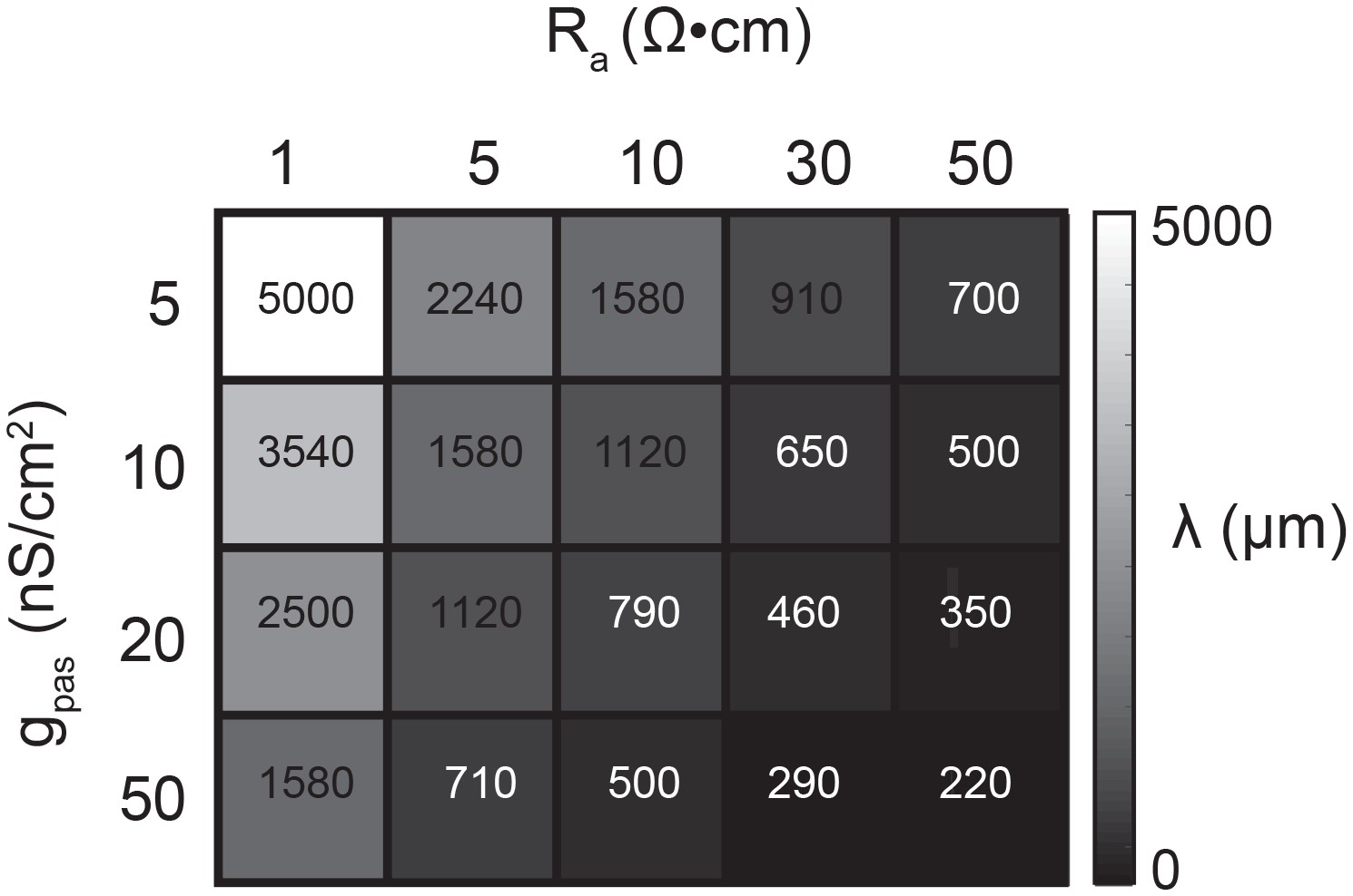
Passive parameters used for cable model library.
All pairwise combinations. of passive conductance (gpas; 5, 10, 20, 50 nS/cm2) and axial resistance (Ra; 1, 5, 10,. 30, 50 Ω•cm) values were used to generate a library of 20 cable models with varying. electrotonic length constants (λ; shown numerically and in gray scale, in microns, as grid. elements below) between 220 µm and 5 mm.
Tables
Table 1
Linear regression analysis for response amplitudes as a function of distance, branch order, and neurite diameter. Each row corresponds to a different GM neuron, with same color scheme, as shown in Figure 5 and Figure 5—figure supplement 1. Note insignificant p values suggesting no dependence of the response amplitude on these cable properties. n corresponds to the number of photo-uncaging sites in each GM neuron.
Distance | Branch order | Diameter | |||||||||||
|---|---|---|---|---|---|---|---|---|---|---|---|---|---|
Neuron | MSE | R | p | slope (mV/um) | MSE | R | p | slope (mV/order) | MSE | R | p | slope (mV/um) | n |
 | 0.11 | −0.27 | 0.418 | −0.0009 | 0.12 | −0.20 | 0.55 | −0.0104 | 0.10 | 0.39 | 0.24 | 0.1028 | 11 |
 | 0.02 | 0.28 | 0.592 | 0.0003 | 0.02 | 0.26 | 0.62 | 0.0052 | 0.03 | 0.01 | 0.99 | 0.0007 | 7 |
 | 0.03 | −0.19 | 0.656 | −0.0003 | 0.03 | −0.21 | 0.62 | −0.0057 | 0.02 | −0.44 | 0.28 | −0.0331 | 9 |
 | 0.59 | 0.42 | 0.229 | 0.0026 | 0.51 | 0.54 | 0.11 | 0.0472 | 0.57 | −0.45 | 0.19 | −0.1713 | 11 |
 | 0.14 | 0.22 | 0.679 | 0.0005 | 0.14 | 0.23 | 0.66 | 0.0100 | 0.12 | −0.48 | 0.33 | −0.0680 | 7 |
 | 0.01 | 0.90 | 0.002 | 0.0013 | 0.02 | 0.68 | 0.07 | 0.0232 | 0.01 | −0.75 | 0.03 | −0.0728 | 9 |
 | 0.02 | -−0.49 | 0.269 | −0.0005 | 0.03 | −0.44 | 0.33 | −0.0073 | 0.03 | 0.32 | 0.48 | 0.0338 | 8 |
 | 0.11 | 0.20 | 0.443 | 0.0008 | 0.11 | 0.24 | 0.35 | 0.0142 | 0.10 | −0.37 | 0.14 | −0.0682 | 18 |
 | 0.02 | 0.26 | 0.579 | 0.0004 | 0.02 | 0.32 | 0.49 | 0.0060 | 0.01 | −0.60 | 0.16 | −0.0244 | 8 |
 | 0.32 | −0.27 | 0.477 | −0.0021 | 0.25 | −0.53 | 0.15 | −0.0455 | 0.25 | 0.51 | 0.16 | 0.3891 | 11 |
Mean | 0.14 | 0.11 | 0.434 | 0.0002 | 0.12 | 0.09 | 0.39 | 0.0037 | 0.12 | −0.19 | 0.30 | 0.0089 | |
SD | 0.18 | 0.41 | 0.214 | 0.0013 | 0.15 | 0.41 | 0.23 | 0.0242 | 0.17 | 0.45 | 0.27 | 0.1520 | |
Table 2
Linear regression analysis for reversal potentials as a function of distance, branch order, and neurite diameter. Each row corresponds to a different GM neuron, with same color scheme, as shown in Figure 8 and Figure 8—figure supplement 1. Note slopes of nearly zero across all 10 neurons, suggesting invariant reversal potentials across the neuronal structure. n corresponds to the number of photo-uncaging sites in each GM neuron.
Reversal potentials | Distance | Branch order | Diameter | ||||||||||||||
|---|---|---|---|---|---|---|---|---|---|---|---|---|---|---|---|---|---|
Neuron | Mean (mV) | SD | CV | MSE | R | p | slope (mV/um) | MSE | R | p | slope (mV/order) | MSE | R | p | slope (mV/um) | n | Rinput (MΩ) |
 | −73.8 | 2.9 | −0.04 | 5.99 | 0.44 | 0.18 | 0.012 | 6.52 | 0.35 | 0.30 | 0.139 | 6.52 | 0.34 | 0.30 | 0.712 | 11 | 10 |
 | −79.2 | 1.2 | −0.02 | 1.21 | 0.00 | 0.99 | 0.000 | 1.16 | −0.21 | 0.68 | −0.029 | 0.54 | −0.75 | 0.09 | −0.513 | 6 | 15 |
 | −81.9 | 3.2 | −0.04 | 8.80 | 0.14 | 0.76 | 0.006 | 8.86 | 0.12 | 0.80 | 0.071 | 5.86 | −0.59 | 0.16 | −1.123 | 7 | 12 |
 | −83.6 | 4.3 | −0.05 | 13.13 | 0.45 | 0.23 | 0.013 | 13.35 | 0.43 | 0.24 | 0.175 | 14.39 | −0.35 | 0.35 | −0.613 | 9 | 12 |
 | −75.6 | 3.8 | −0.05 | 9.42 | 0.15 | 0.90 | 0.0010 | 9.61 | -0.05 | 0.97 | −0.058 | 0.34 | −0.98 | 0.12 | −10.756 | 3 | 11 |
 | −87.7 | 2.7 | −0.03 | 5.18 | 0.34 | 0.51 | 0.009 | 5.27 | 0.32 | 0.54 | 0.142 | 5.20 | 0.34 | 0.51 | 0.478 | 6 | 7 |
 | −64.8 | 3.6 | −0.06 | 8.59 | −0.50 | 0.26 | −0.011 | 7.53 | −0.58 | 0.17 | −0.185 | 11.38 | −0.04 | 0.93 | −0.084 | 7 | 5 |
 | −69.9 | 3.3 | −0.05 | 9.37 | −0.22 | 0.46 | −0.008 | 9.01 | −0.29 | 0.33 | −0.146 | 9.84 | 0.05 | 0.87 | 0.015 | 11 | 7 |
 | −84.6 | 3.0 | −0.04 | 7.88 | -−0.02 | 0.97 | −0.001 | 7.80 | 0.10 | 00.83 | 0.039 | 7.88 | −0.0 | 0.96 | −0.020 | 7 | 10 |
 | −85.0 | 2.2 | −0.03 | 3.02 | −0.53 | 0.28 | −0.042 | 4.11 | 0.13 | 0.80 | 0.144 | 2.84 | 0.57 | 0.24 | 1.805 | 6 | 10 |
Pooled Mean | −78.6 | −0.04 | 7.26 | 0.03 | 0.55 | −0.001 | 7.32 | 0.03 | 0.57 | 0.029 | 6.48 | −0.14 | 0.45 | −1.010 | 9.9 | ||
Pooled SD | 7.4 | 3.47 | 0.35 | 0.32 | 0.016 | 3.34 | 0.32 | 0.29 | 0.128 | 4.57 | 0.51 | 0.34 | 3.518 | 2.9 | |||
Additional files
-
Supplementary file 1
Neuronal Structure Hoc files.
- https://doi.org/10.7554/eLife.23508.020
-
Supplementary file 2
Uncaging Coordinates Hoc files.
- https://doi.org/10.7554/eLife.23508.021
Download links
A two-part list of links to download the article, or parts of the article, in various formats.
Downloads (link to download the article as PDF)
Open citations (links to open the citations from this article in various online reference manager services)
Cite this article (links to download the citations from this article in formats compatible with various reference manager tools)
When complex neuronal structures may not matter
eLife 6:e23508.
https://doi.org/10.7554/eLife.23508


