Ketamine induces multiple individually distinct whole-brain functional connectivity signatures
- Department of Psychiatry, Yale University School of Medicine, United States
- Department of Psychiatry, Psychotherapy and Psychosomatics, University Hospital for Psychiatry Zurich, Switzerland
- Department of Physics, Yale University, United States
- David Geffen School of Medicine, University of California, Los Angeles, United States
- Interdepartmental Neuroscience Program, Yale University, United States
- Department of Psychiatry, University of Zagreb, Croatia
- Department of Psychology, University of California, Los Angeles, United States
- Center of Neuroscience, University of Pittsburgh, United States
- Department of Psychiatry, Vanderbilt University Medical Center, United States
- Magnetic Resonance Research Center, Yale University School of Medicine, United States
- Department of Radiology and Psychiatry, Baylor College of Medicine, United States
- Child Study Center, Yale University School of Medicine, United States
- Department of Psychology, University of Ljubljana, Slovenia
- Department of Psychiatry, Bridgeport Hospital, United States
- Department of Psychology, Yale University, United States
Figures
Figure 1 with 5 supplements
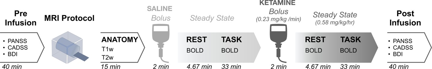
Neuroimaging protocol.
The study employed a single-blind within-subjects design, with participants blinded to their treatment condition. Forty participants received an IV cannulation in each forearm: one IV for the placebo/ketamine infusion and one for blood draws during the scan. Placebo was administered during the first neuroimaging can session, and ketamine (initial bolus 0.23 mg/kg, continuous infusion 0.58 mg/kg/hr) during the second because residual ketamine effects ruled out counterbalancing of the order. Blood was drawn immediately after the resting-state run. Cognitive effects were measured using a Spatial Working Memory task completed in the scanner. Subjective effects were measured 180 min post drug administration using the following scales: (1) Positive and Negative Syndrome Scale (PANSS), (2) Clinician Administered Dissociative States Scale (CADSS), and (3) Beck’s Depression Inventory (BDI).
Figure 1—figure supplement 1

Mean effect of ketamine on global brain connectivity without global signal regression.
(A-B) Placebomean GBC neural mFz-value map at the grayordinate level (left, no. grayordinates = 91281) and parcel level (right). (C-D) Ketamine mean GBC neural mFz-value map at the grayordinate level (left) and parcel level (right). (E-F) Mean Δ (ketamine - placebo) GBC neural mFz-value map at thegrayordinate level (left) and parcel level (right). (G-H) Ketamine vs. placebo t-test unthresholded Z-score map at the grayordinate level (left) and parcel level (right). Red/orange areas indicate regions where participants exhibited stronger GBC in the ketamine condition, whereas blue areas indicate regions where participants exhibited reduced GBC in the ketamine condition. (I-J) Ketamine vs. placebo t-test significant (FDR protected, 5000 permutations) areas showing increased (red) and decreased (blue) GBC in the ketamine condition compared to placebo at the grayordinatelevel (left) and parcel level (right). (K) Scatter plots showing the relationship between the mean Δ GBC mFz-value map and the unthresholded t-test Δ GBC Z-score map (Z-scores computed across 718 parcels) at the grayordinate level (left) and parcel level (right). (L) Correlation matrix showingthe relationship between mean Δ GBC map and t-test Δ GBC map with and without GSR at the grayordinate level (left) and parcel level (right).
Figure 1—figure supplement 2
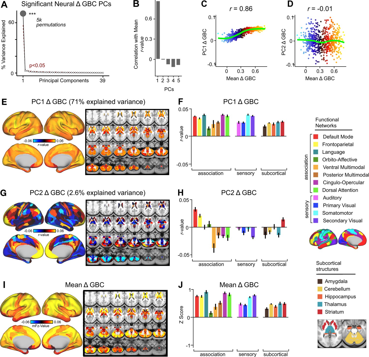
Multi-dimensional neural effect of acute ketamine administration without global signal regression.
(A) Results of PCA performed on Δ GBC neural features without global signal regression (GSR) (718 whole-brain parcel GBC) across all subjects (N=40). Screeplot showing the % variance explained by the 39 Δ GBC PCs. The first Δ GBC PC (dark grey) was determined to be significant using a permutation test (p<.05, 5000 permutations). PC1 Δ GBC captures 71% of the total variance in neural GBC in the sample. (B) Bar plot showing the correlation between the first five Δ GBC PCs and the mean Δ GBC. PC1 Δ GBC is most highly correlated with mean Δ GBC, which is to be expected as PC1 Δ GBC explains the largest amount of variance in the neural data and is the only significant PC. (C) Scatter plot showing the relationship across parcels between mean Δ GBC and PC1 Δ GBC maps (r=0.86, p<.001, N=718). Green line indicates that while the positive valuesare correlated, the negative values do not correlate. (D) Scatter plot showing the relationship across parcels between mean Δ GBC and PC2 Δ GBC maps (r=-0.01, p>.05, N=718). Green line indicates neither the positive or negative values are highly correlated. (E) PC1 Δ GBC r-value map.PC1 Δ GBC explains 71% of all variance. Red/orange areas indicate parcels that have a high positive loading score onto PC1, while blue areas indicate parcels that have a high negative loading score onto PC1. (F) Bar plot showing the mean correlation (Δ GBC, PC1 score) for each network and each anatomical subcortical structure for PC1 Δ GBC (see inset right for color labels). (G) PC2 Δ GBC r-value map. PC2 Δ GBC explains 2.6% of all variance. Red/orange areas indicate parcels that have a high positive loading score onto PC2, while blue areas indicate parcels that havea high negative loading score onto PC2. (H) Bar plot showing the mean correlation (Δ GBC, PC2 score) for each network and each anatomical subcortical structure for PC2 Δ GBC (see inset right for color labels). (I) Unthresholded mean Δ GBC mFz-value map. Red/orange areas indicate regions where participants exhibited stronger GBC in the ketamine condition, whereas blue areas indicate regions where participants exhibited reduced GBC in the ketamine condition, compared with the placebo condition. (J) Bar plot showing the mean Δ GBC mFz-value for each network and each anatomical subcortical structure for mean Δ GBC (see inset right for color labels).
Figure 1—figure supplement 3
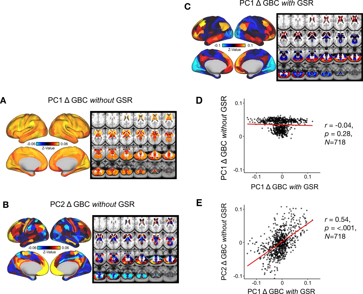
Comparison of Delta GBC Principal Component Analysis (PCA) with vs. without Global Signal Regression(GSR).
(A) PC1 Δ GBC z-value map without GSR. PC1 Δ GBC without GSR explains 71% of all variance. Red/orange areas indicate parcels that have a high positive loading score onto PC1, while blue areas indicate parcels that have a high negative loading score onto PC1. (B) PC2 Δ GBCz-value map without GSR. PC2 Δ GBC without GSR explains 2.6% of all variance. Red/orange areas indicate parcels that have a high positive loading score onto PC2, while blue areas indicate parcels that have a high negative loading score onto PC2. (C) PC1 Δ GBC Z-score map with GSR (Z-scores computed across 718 parcels). PC1 Δ GBC with GSR explains 14.1% of all variance. Red/orange areas indicate parcels that have a high positive loading score onto PC1, while blue areas indicate parcels that have a high negative loading score onto PC1. (PC1 is sign flipped for visual comparison with mean). (D) Scatter plot showing the correlation across parcels (N=718) between PC1 Δ GBC Z-score map with GSR and PC1 ΔGBC Z-score map without GSR (Z-scores computed across 718 parcels). (E) Scatter plot showing the correlation across parcels (N=718) between PC1 Δ GBC Z-score map with GSR and PC2 Δ GBC Z-score map without GSR (Z-scores computed across 718 parcels).
Figure 1—figure supplement 4
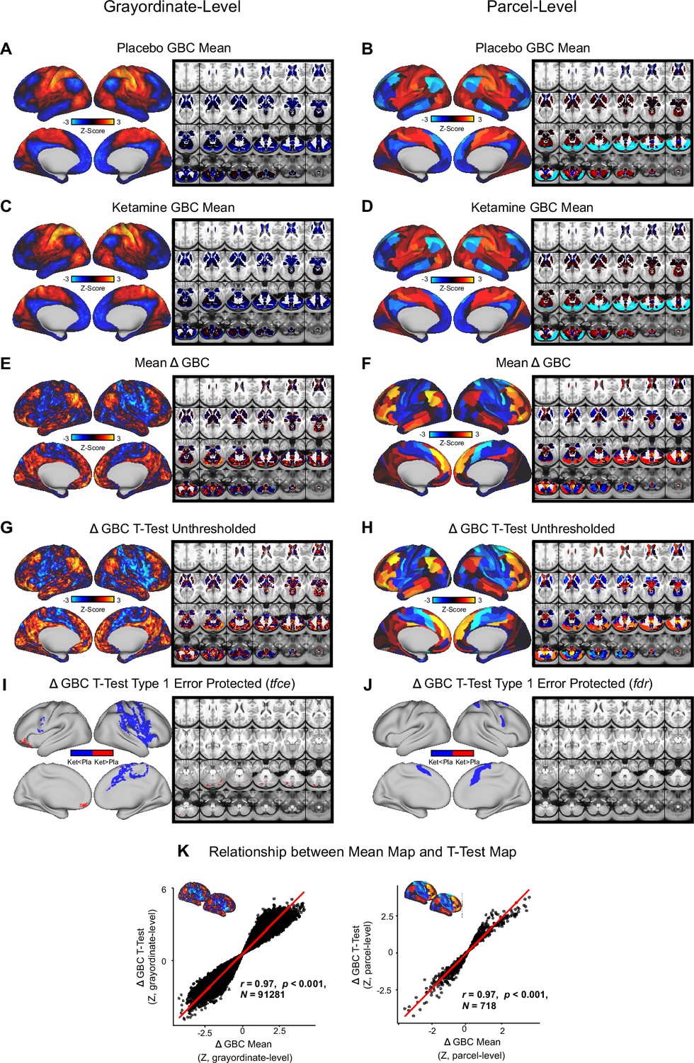
Mean effect of ketamine on GBC.
(A-B) Placebo mean GBC neural map at the gray ordinate level (left, no.gray ordinates = 91281) and parcel level (right). (C-D) Ketamine mean GBC neural map at the gray ordinate level (left) and parcel level (right). (E-F) Mean Δ (ketamine - placebo) GBC neural map at the gray ordinate level (left) and parcel level (right). (G-H) Ketamine vs. placebo t-test unthresh-olded Z-score map at the gray ordinate level (left) and parcel level (right). Red/orange areas indicate regions where participants exhibited stronger GBC in the ketamine condition, whereas blue areas indicate regions where participants exhibited reduced GBC in the ketamine condition. (I-J) Ketamine vs. placebo t-test significant (threshold free cluster enhancement type 1 error protected, 5000 permutations) areas showing increased (red) and decreased (blue) GBC in the ketamine condition compared to placebo at the gray ordinate level (left) and parcel level (right). (K) Scatter-plots showing the relationship between the mean Δ GBC map and the unthresholded t-test Δ GBC map at the grayordinate level (left) and parcellevel (right).
Figure 1—figure supplement 5
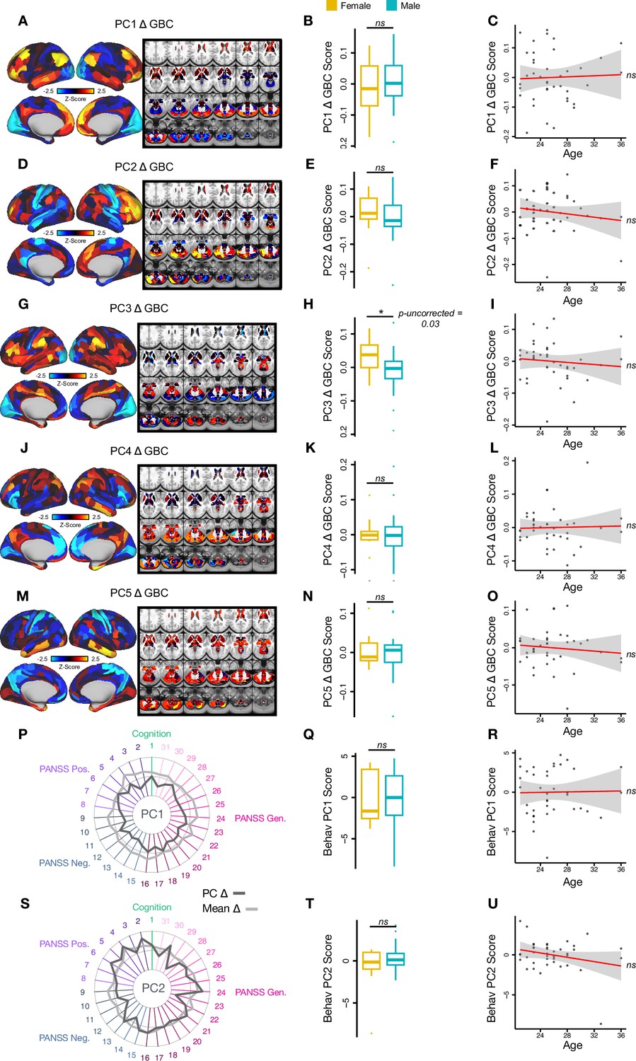
Effect of sex and age on neural and behavioral PC scores.
(A, D, G, J, M) Neural PC 1-5 Δ GBC maps. (B, E, H, K, N) Differences between women (yellow) and men’s (blue) neural PC 1-5 Δ GBC scores. (C, F, I, L, O) Correlation between age and neural PC 1-5 Δ GBC scores. (P, S) Behavioral PC 1-2. (Q, T) Differences between women (yellow) and men’s (blue) behavioral PC 1-2 scores. (R, U) Correlation between age and behavioral PC 1-2 scores.
Figure 2 with 7 supplements
Multidimensional neural effect of acute ketamine administration.
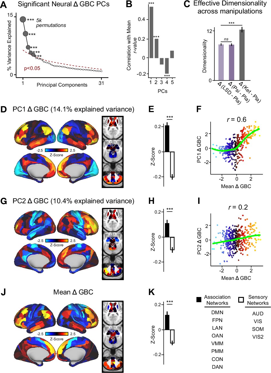
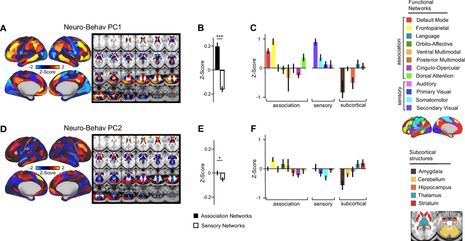
(A) Results of PCA performed on Δ GBC neural features (718 whole-brain parcel GBC) across all subjects (N=40). Screeplot showing the % variance explained by the first 31 (out of 39) Δ GBC PCs. The first 5 Δ GBC PCs (dark gray) were determined to be significant using a permutation test (p<0.05, 5000 permutations). The size of each dark gray point is proportionate to the variance explained. Together, these 5 Δ GBC PCs capture 42.1% of the total variance in neural GBC in the sample. (B) Bar plot showing the correlation between each of the five significant Δ GBC PCs maps and the mean Δ GBC map. r values for PC1, PC2, and PC4 Δ GBC are significant (***=p < 0.001, Bonferroni corrected). (C) Bar plot showing the effective dimensionality across three pharmacological conditions: Δ LSD (LSD - placebo), Δ psilocybin (psilocybin - placebo), and Δ ketamine (ketamine - placebo). (Light purple = LSD, dark purple = psilocybin, dark gray = ketamine). There was a statistically significant difference between groups as determined by a one-way ANOVA (F(2,60)=564, p<0.001). Post hoc tests revealed that dimensionality was significantly lower in the LSD (8.7+/-0.3, p<0.001) and the psilocybin (8.6+/-0.3, p<0.001) conditions compared to the ketamine (12.8±0.7) condition. There was no statistically significant difference in dimensionality between LSD and psilocybin (p=0.6). Error bars = standard deviation. (D) Unthresholded PC1 Δ GBC Z-score map (Z-scores computed across 718 parcels). PC1 Δ GBC explains 14.1% of all variance. Red/orange areas = parcels that have a high positive loading score onto PC1, blue areas = parcels that have a high negative loading score onto PC1. (E) Bar plot showing the PC1 Δ GBC Z-score across association (black) and sensory (white) network parcels. (F) Scatter plot showing the relationship across parcels between mean Δ GBC and PC1 Δ GBC maps (r=0.56, p<0.001, n=718). (G) Unthresholded PC2 Δ GBC Z-score map (Z-scores computed across 718 parcels). PC2 Δ GBC explains 10.4% of all variance. Red/orange areas = parcels that have a high positive loading score onto PC2, blue areas = parcels that have a high negative loading score onto PC2. (H) Bar plot showing the PC2 Δ GBC Z score across association (black) and sensory (white) network parcels. (I) Scatter plot showing the relationship across parcels between mean Δ GBC and PC2 Δ GBC maps (r=0.23, p<0.001, n=718). Green line indicates neither the positive or negative values are highly correlated. (J) Unthresholded mean Δ (ketamine - placebo) GBC Z-score map (Z-scores computed across 718 parcels). Red/orange areas = parcels where participants exhibited stronger GBC in the ketamine vs. placebo condition, blue areas = parcels where participants exhibited reduced GBC in the ketamine vs. placebo condition. (K) Bar plot showing the mean Δ GBC Z-score across association (black) and sensory (white) network parcels. (DMN = default mode, FPN = frontoparietal, LAN = language, OAN = orbito-affective, VMM = ventro multimodal, PMM = posterior multimodal, CON = cingulo-opercular, DAN = dorsal attention, AUD = auditory, VIS = primary visual, SOM = somatomotor, VIS2=secondary visual).
Figure 2—figure supplement 1
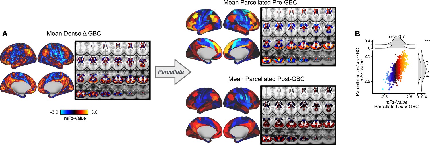
Parcellating before running GBC results in an improved signal to noise ratio.
(A) (Left) Unthresholded Δ (ketamine - placebo) GBC mean map at the grayordinate-level. (Right) Unthresholded Δ GBC mean map parcellated before running GBC (top) or after (bottom) running GBC. (B) Scatter plot showing relationship between parcel values (GBC mFz-values) computed pre vs. post GBC. Marginal distribution plots show the variance of Δ GBC mean map parcellated before GBC (σ2 = 1.9, right) and the variance of Δ GBC mean map parcellated before GBC (σ2 = 0.7, top). A paired Pitman-Morgan test revealed that there is a significant difference in variance between the two maps (p<0.001).
Figure 2—figure supplement 2
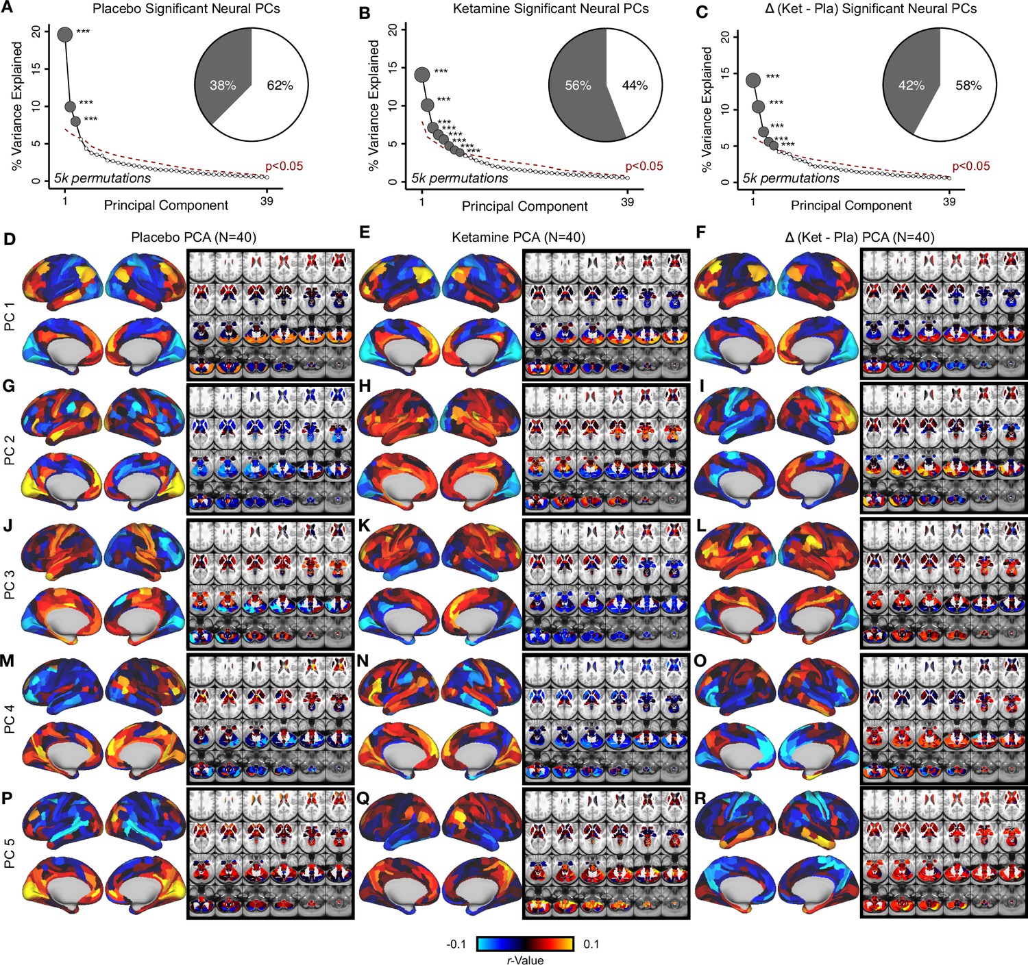
Principal component analysis (PCA) on the neural features from the placebo, ketamine, and Δ (ketamine- placebo) neural GBC maps.
(A) Screeplot showing the total proportion of variance explained by the 39 PCs from the PCA performed acrossall 718 neural features in 40 subjects in the placebo condition. The size of each gray point is proportional to the variance explained by that PC. The first 3 gray PCs were determined to be significant using a permutation test (5000 permutations). Inset shows the proportion of variance both accounted and not accounted for by the 3 PCs. Together, these 3 PCs captures 37.5% of the total variation in neural GBC in the sample. (B) Screeplot showing the total proportion of variance explained by the 39 PCs from the PCA performed across all 718 neural features in 40 subjectsin the ketamine condition. The size of each gray point is proportional to the variance explained by that PC. The first 8 gray PCs were determined to be significant using a permutation test 5000 permutations. Inset shows the proportion of variance both accounted and not accounted for by the 8 PCs. Together, these 8 PCs captures 55.8% of the total variation in neural GBC in the sample. (C) Screeplot showing the total proportion of variance explained by the 39 PCs from the PCA performed across all 718 neural features in 40 subjects in the Δ condition. The size of each gray point is proportional to the variance explained by that PC. The first 5 gray PCs were determined to be significant using a permutation test (5000 permutations). Inset shows the proportion of variance both accounted and not accounted for by the 5 PCs. Together, these 5 PCs captures 42.1% of the total variation in neural GBC in the sample. (D-R) Neural maps for PC1-5 from the PCA performed on neural features (718 whole-brain parcel GBC) across all subjects in the placebo (left column), ketamine (centre column), and Δ (ketamine - placebo) conditions (right column). Red/orange areas indicate parcels that have a high positive loading score onto the PC, while blue areas indicate parcels that have a high negative loading score onto the PC.
Figure 2—figure supplement 3

Individual variation in PC1-5 Δ GBC and mean Δ GBC.
(A, C, E, G, I) Unthresholded PC1-5 Δ GBC Z-score map (Z-scores computed across 718 parcels). Red/orange areas indicate parcels that have a high positive loading score onto PC1, while blue areas indicate parcels that have a high negative loading score onto PC1. (PC1 and PC2 are sign flipped for visual comparison with mean). (B, D, F, H, J) (Left) Bar plot showing the PC1-5 Δ GBC score (r-value) for each participant (N=40). The score for each participant was calculated by correlating their individual Δ GBC map with the PC Δ GBC map. (Right) density plot showing the variation captured by each PC Δ GBC. (K) Unthresholded mean Δ (ketamine - placebo) GBC Z-score map (Z-scores computed across 718 parcels). Red/orange areas indicate regions where participants exhibited stronger GBC in the ketamine condition, whereas blue areas indicate regions where participants exhibited reduced GBC in the ketamine condition, compared with the placebo condition. (L) (Left) Bar plot showing the mean Δ GBC score (r-value) for each participant (N=40). The score for each participant was calculated by correlating their individual Δ GBC map with the mean Δ GBC map. (Right) density plot showing the variation captured by the mean Δ GBC.
Figure 2—figure supplement 4

Network breakdown of PC1-5 Δ GBC and mean Δ GBC.
(A, D, G, J, M) Unthresholded PC1-5 Δ GBC Z-score map (Z-scores computed across 718 parcels). Red/orange areas indicate parcels that have a high positive loading score onto the PC, while blue areas indicate parcels that have a high negative loading score onto the PC. (PC1 and PC2 are sign flipped for visual comparison with mean). (B, E, H, K, N) Bar plot showing the PC1-5 Δ GBC Z-score across association (black) and sensory (white) network parcels. See graphs right for association andsensory network groupings. (C, F, I, L, O) Bar plot showing the mean Z-score for each network and each anatomical subcortical structure for PC1-5Δ GBC (see inset right for color labels). Networks are grouped into association and sensory networks. (P) Unthresholded mean Δ (ketamine -placebo) GBC Z-score map (Z-scores computed across 718 parcels). Red/orange areas indicate regions where participants exhibited stronger GBC in the ketamine condition, whereas blue areas indicate regions where participants exhibited reduced GBC in the ketamine condition, compared with the placebo condition. (Q) Bar plot showing the mean Δ GBC Z-score across association (black) and sensory (white) network parcels. See graphs right for association and sensory network groupings. (R) Bar plot showing the mean Z-score for each network and each anatomical subcortical structure for mean Δ GBC (see inset right for color labels). Networks are grouped into association and sensory networks.
Figure 2—figure supplement 5
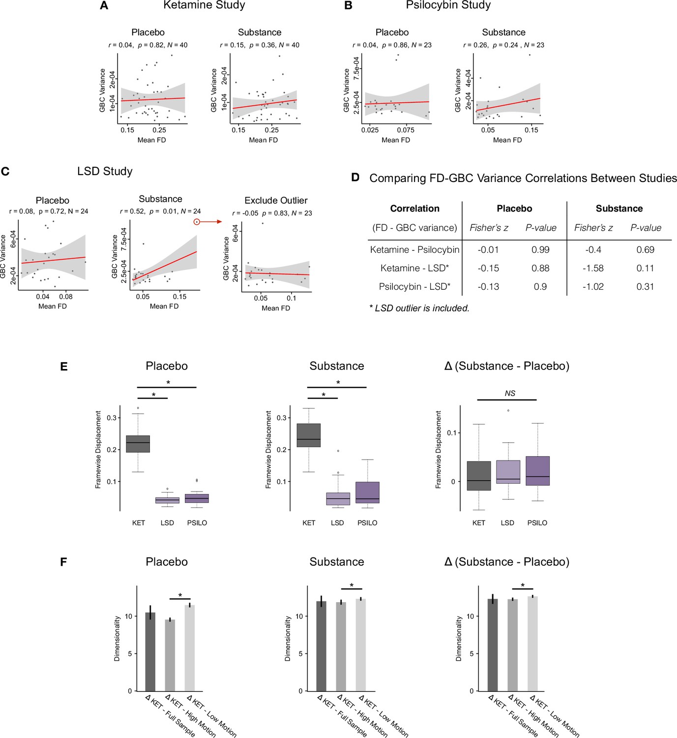
Investigating the relationship between motion, GBC variance, and effective dimensionality across threedatasets: ketamine, LSD, and psilocybin.
(A-B) We found no relationship between mean framewise displacement (FD) and GBC variance for the placebo or substance scan sessions for the ketamine or psilocybin studies. (C) In the LSD study we found no relationship between mean FD and GBC variance for the placebo scan session (left), but we did find a positive correlation between mean FD and GBC variance for the substance sessions (r=0.52, p=0.01) (centre). However, this correlation is driven by a single outlier which when removed results in a non-significant correlation (r=-0.05, p=0.83) (right). (D) When we compared the correlations between mean FD and mean GBC across all three studies using Fisher-Z-Transformation, we found no difference in correlations between any of the studies (LSD outlier left in). (E) We directly compared FD in each of the three studies, and found that while FD in both the placebo (left) and substance (centre) scan sessions was significantly higherin the ketamine study compared to the LSD and psilocybin study, we found no difference in Δ (substance - placebo) FD (right) between the three studies. Δ (substance - placebo) is the input for the analyses throughout the manuscript. (F) Given we see ketamine shows higher effective dimensionality compared to LSD and psilocybin, and ketamine shows increased FD compared to LSD and psilocybin in the placebo and substance scan sessions,we wanted to investigate whether ketamine’s higher FD could be related to its higher effective dimensionality score. To explore this, we separated the ketamine study participants into those with the higher FD values (i.e. the ’high motion’ group) and those with the lower FD values (i.e. the ’low motion’ group). We then calculated effective dimensionality for the high and low motion groups, and found that effective dimensionality was significantly higher in the low motion group compared to the high motion group for the placebo, substance, and Δ scan sessions. This indicates that the higher motion seen in the ketamine study is not what is driving its higher effective dimensionality score as here we see the opposite pattern: effective dimensionality is higher in the low motion group.
Figure 2—figure supplement 6
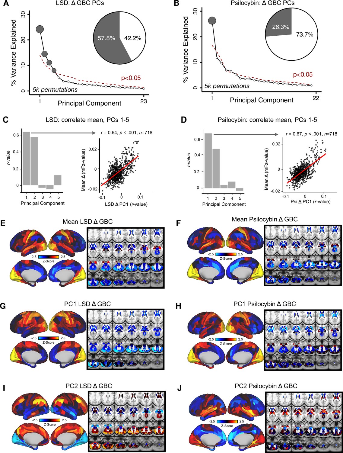
Principal Component Analysis of LSD and psilocybin Δ GBC.
(A) Results of PCA performed on Δ (LSD - placebo)GBC neural features (718 whole-brain parcel GBC) across all subjects (N=24). Screeplot showing the % variance explained by the each of the 23 PCs. The first 4 PCs (dark grey) were determined to be significant using a permutation test (p<.05, 5000 permutations). The size of each dark grey point is proportionate to the variance explained. Inset shows the proportion of variance both accounted and not accounted for by the 4 PCs. (B) Results of PCA performed on Δ (psilocybin - placebo) GBC neural features (718 whole-brain parcel GBC) across all subjects (N=23). Screeplot showing the % variance explained by the each of the 22 PCs. The first PC (dark grey) was determined to be significant using a permutation test (p<.05, 5000 permutations). The size of the dark grey point is proportionate to the variance explained. Inset shows the proportion of variance both accounted and not accounted for by the PC. The single PC captures 26.3% of the total variation in neural GBC in the sample. (C) Bar plot showing the correlation between each of the first five LSD Δ GBC PCs and the mean LSD Δ GBC. r values for PC1 and PC2 are significant (p<.001,Bonferroni corrected). (Inset) Scatter plot showing the relationship across parcels between mean LSD Δ GBC and PC1 LSD Δ GBC maps. (D) Barplot showing the correlation between each of the first five psilocybin Δ GBC PCs and the mean psilocybin Δ GBC map. r values for PC1 andPC2 are significant (p<.001, Bonferroni corrected). (Inset) Scatter plot showing the relationship across parcels between mean psilocybin Δ GBCand PC1 psilocybin Δ GBC maps. (E) Unthresholded mean LSD Δ GBC Z-score map at the parcel level (No. parcels = 718) (Z-scores computed across 718 parcels). Red/orange areas indicate regions where participants exhibited stronger GBC in the LSD condition, whereas blue areas indicate regions where participants exhibited reduced GBC in the LSD condition, compared with the placebo condition. (F) Unthresholded mean psilocybin Δ GBC Z-score map at the parcel level (No. parcels = 718) (Z-scores computed across 718 parcels). Red/orange areas indicate regions where participants exhibited stronger GBC in the psilocybin condition, whereas blue areas indicate regions where participants exhibited reduced GBC in the psilocybin condition, compared with the placebo condition. (G) PC1 LSD Δ GBC Z-score map (Z-scores computed across 718 parcels). PC1 LSD Δ GBC explains 25% of all variance. Red/orange areas indicate parcels that have a high positive loading score onto PC1, while blue areas indicate parcels that have a high negative loading score onto PC1. (PC1 is sign flipped for visual comparison with mean). (H) PC1 psilocybin Δ GBC Z-score map (Z-scores computed across 718 parcels). PC2 Δ GBC explains 26.3% of all variance. Red/orange areas indicate parcels that have a high positive loading score onto the PC2, while blue areas indicate parcels that have a high negative loading score onto the PC2. (I) PC2 LSD Δ GBCZ-score map (Z-scores computed across 718 parcels). (J) PC2 psilocybin Δ GBC Z-score map (Z-scores computed across 718 parcels).
Figure 2—figure supplement 7
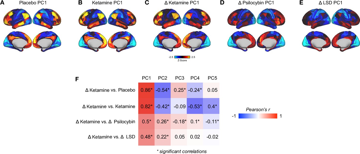
A comparison of principal component analysis results across the following datasets: placebo, ketamine, Δ, Δ psilocybin, and Δ LSD.
All results are computed at the parcel-level (no. parcels = 718) (z-scores computed across 718 parcels). (A) Unthresholded placebo GBC PC1 Z-score map. (B) Unthresholded ketamine GBC PC1 Z-score map. (C) Unthresholded ketamine Δ GBC PC1 Z-score map. Δ = ketamine - placebo. (D) Unthresholded psilocybin Δ GBC PC1 Z-score map. Δ = psilocybin - placebo. (E) Unthresholded LSD Δ GBC PC1 Z-scoremap. Δ = LSD - placebo. (F) Correlations across PC1-5 for: top row = Δ ketamine and placebo, second row = Δ ketamine and ketamine, third row = Δ ketamine and Δ psilocybin, fourth row = Δ ketamine and Δ LSD. * denotes significant correlations (P-corrected < 0.05). The moderate correlations between Δ ketamine PC1 and Δ psilocybin PC1 /Δ LSD PC1 demonstrate that the findings do show specificity to the ketamine-placebo contrast, although a thorough comparison of the PCA results across substances is beyond the scope of this manuscript.
Figure 3 with 2 supplements
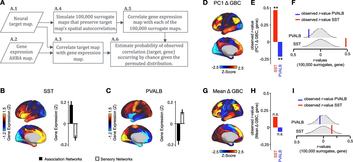
PC1 Δ GBC map is associated with SST and PVALB cortical gene expression patterns.
(A) Gene analysis workflow. (A.1) Selection of neural target map. (A.2) Cortical gene expression map was obtained using GEMINI-DOT (Burt et al., 2018). Specifically, an AHBA gene expression map was obtained using DNA microarrays from six postmortem human brains, capturing gene expression topography across cortical areas. These expression patterns were then mapped onto the cortical surface models derived from the AHBA subjects’ anatomical scans and aligned with the Human Connectome Project (HCP) atlas, described in prior work and Methods (Burt et al., 2018). (A.3) Correlation of the neural target map with the gene expression map to obtain the observed r value. (A.4) To calculate the significance of the observed r value, we first used BrainSMASH (Burt et al., 2020) to simulate 100,000 surrogate maps that preserve the neural target map’s spatial autocorrelation. (A.5) We then correlated the gene expression map with each of the 100,000 surrogate maps, to generate a distribution of 100,000 simulated r values. (A.6) Finally, we estimated the probability of the observed correlation between the neural target map and the gene expression map occurring by chance given the permuted distribution. For further details see (Figure 2—figure supplement 2) (B) Gene expression pattern for interneuron marker gene somatostatin (SST). Left: positive (yellow) regions show areas where the gene of interest is highly expressed, whereas negative (blue) regions indicate low expression values. Right: bar plot showing the mean gene expression Z-score across association (black) and sensory (white) networks. (C) Gene expression pattern for interneuron marker parvalbumin (PVALB). Left: positive (yellow) regions show areas where the gene of interest is highly expressed, whereas negative (blue) regions indicate low expression values. Right: bar plot showing the mean gene expression Z-score across association (black) and sensory (white) networks. (D) Unthresholded PC1 Δ GBC Z-score map (Z-scores computed across 718 parcels). Red/orange areas indicate parcels that have a high positive loading score onto PC1, while blue areas indicate parcels that have a high negative loading score onto PC1. (E) Bar plot showing the correlation between PC1 Δ GBC and the following gene expression maps: SST (r=0.47, p<0.001) (red) and PVALB (r=−0.22, p=0.025) (blue). All p-values are FDR corrected. (F) Distribution of 100,000 simulated r values for SST (bottom) and PVALB (top). Bold lines indicate the observed r value between PC1 Δ GBC and SST (red) and PVALB (blue). (G) Unthresholded mean Δ (ketamine - placebo) GBC Z-score map at the parcel level (No. parcels = 718) (Z-scores computed across 718 parcels). Red/orange areas indicate regions where participants exhibited stronger GBC in the ketamine condition, whereas blue areas indicate regions where participants exhibited reduced GBC in the ketamine condition, compared with the placebo condition. (H) Bar plot showing the correlation between mean Δ GBC and the following gene expression maps: SST (r=0.15, p=0.363) (red) and PVALB (r=−0.06, p=0.627) (blue). All p-values are FDR corrected. (I) Distribution of 100,000 simulated r values for SST (bottom) and PVALB (top). Bold lines indicate the observed r value between mean Δ GBC and SST (red) and PVALB (blue).
Figure 3—figure supplement 1

PC1 Δ GBC and PC3-5 Δ GBC maps tracks SST and PVALB neural gene expression patterns.
(A) Gene expression pattern of interneuron marker gene somatostatin (SST). Left: positive (yellow) regions show areas where the gene of interest is highly expressed, whereas negative (blue) regions indicate low expression values. Right: bar plot showing the mean gene expression Z-score across association (black) and sensory (white) networks. (B) Gene expression pattern of inter neuron marker parvalbumin (PVALB). Left: positive (yellow) regions show areas where the gene of interest is highly expressed, whereas negative (blue) regions indicate low expression values. Right: barplot showing the mean gene expression Z-score across association (black) and sensory (white) networks. (C, F, I, L, O) Unthresholded PC1-5 Δ GBCZ-score map (Z-scores computed across 718 parcels). Red/orange areas indicate parcels that have a high positive loading score onto the PC, while blue areas indicate parcels that have a high negative loading score onto the PC. (PC1 and PC2 are sign flipped for visual comparison with mean). (D, G, J, M, P) Bar plots showing the correlation between PC1-5 Δ GBC and the following gene expression maps: SST (red) and PVALB (blue). All p-values are FDR corrected. ** = p<.001, * = p<.05. (E,H,K,N,Q) Distribution of 100,000 simulated r values for SST (bottom) and PVALB (top). Bold lines indicate the observed r value between the PC Δ GBC and SST (red) and PVALB (blue).
Figure 3—figure supplement 2
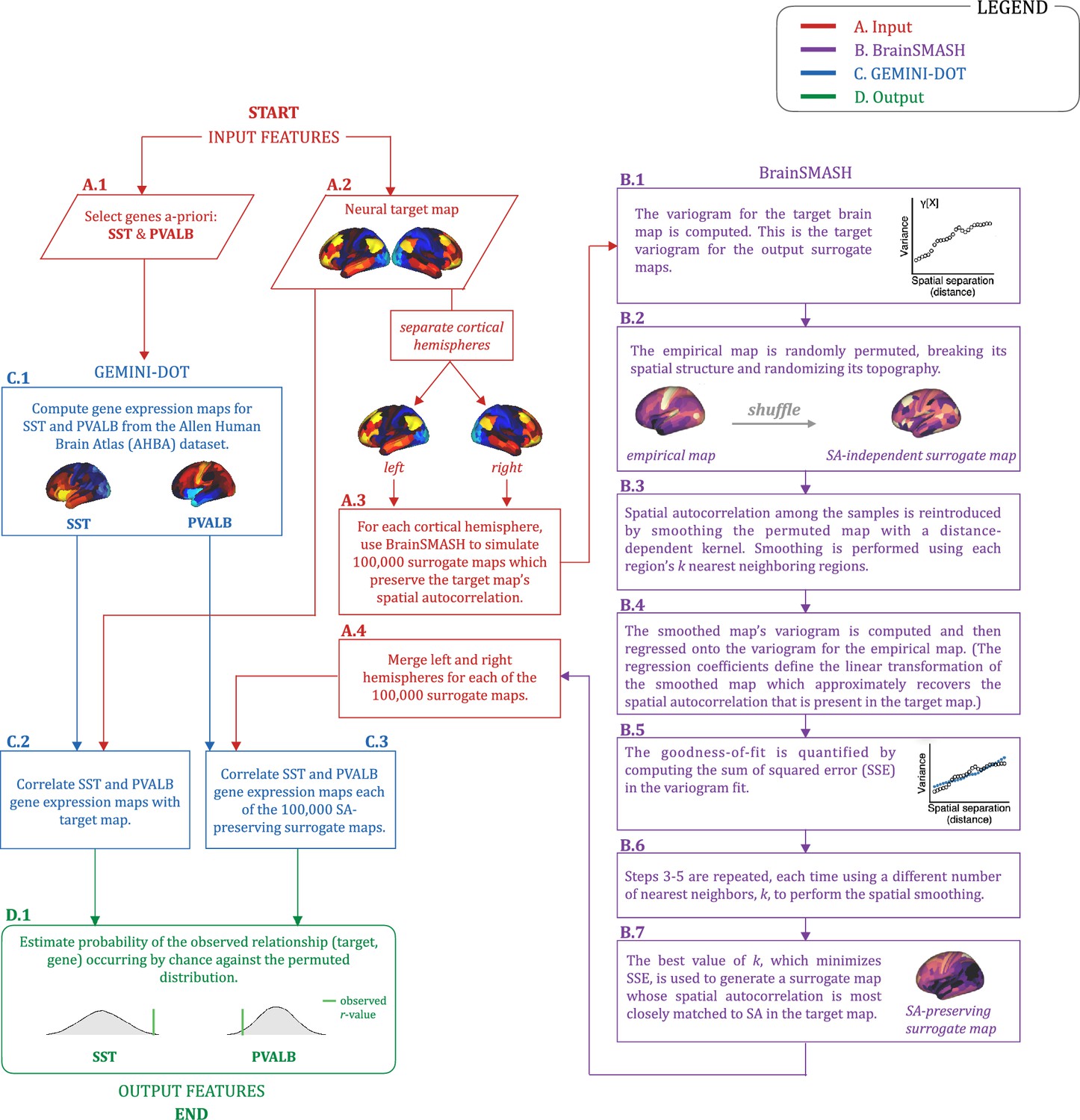
Gene analysis workflow.
Gene analysis workflow outlining: (A.1-2) the input features (red); (B.1-7) the generation of surrogate maps using Brain SMASH (purple); (C.1-3) the generation of gene expression maps using GEMINI-DOT (blue); and (D.1) the ouput features (green).
Figure 4 with 3 supplements
Multidimensional behavioral effect of acute ketamine administration.
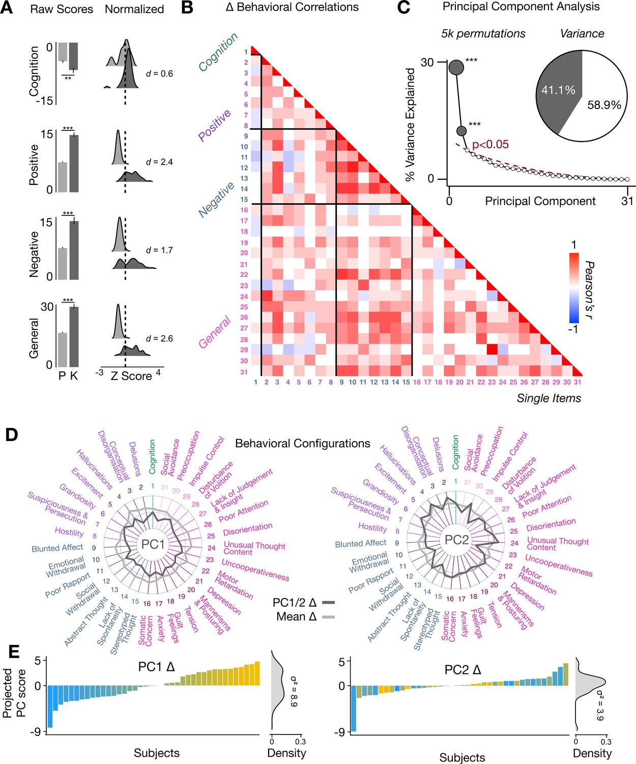
(A) Mean raw scores (left panel) and distribution of normalized scores (right panel) for placebo (P) and ketamine (K) across cognition (spatial working memory) and subjective effects (PANSS positive, PANSS negative, and PANSS general symptoms). Bar plot error bars show standard deviations; distribution plot effect sizes are calculated using Cohen’s d. Condition is color coded (light gray = placebo, dark gray = ketamine). (**=p < 0.05, ***=p < 0.001). For further details see Supplementary file 1. (B) Correlations between 31 individual item behavioral measures for all participants (N=40). Δ (ketamine - placebo) behavioral measures are used. (C) Screeplot showing the % variance explained by each of the principal components (PCs) from a PCA performed using all 31 Δ (ketamine - placebo) behavioral measures across 40 participants. The size of each dark gray point is proportional to the variance explained. The first two PCs (dark gray) survived permutation testing (p<0.05, 5000 permutations). Together they capture 41.1% of all symptom variance (inset), with PC1 explaining 29% of the variance and PC2 explaining 12% of the variance. (D) Loading profiles shown in dark gray across the 31 behavioral items for PC1 Δ (left) and PC2 (right) Δ. See Figure 3—figure supplement 1 for numerical values of the behavioral item scores for each PC. The mean Δ score for each behavioral item is also shown in light gray (scaled to fit the same radar plots). Note that the mean Δ configuration resembles the PC1 Δ loading profile more closely than PC2 Δ (which is to be expected as PC1 explains more variance in the behavioral measures). Inner circle = –0.5, middle circle = 0, outer circle = 0.5. (E) Bar plot showing the projected PC score for each individual subject (N=40) for PC1 Δ (left) and PC2 (right) Δ. Bars are color coded according to each subject’s PC1 score ranking. The density of the projected PC scores is displayed on the right of each bar plot, demonstrating again that PC1 explains the greatest amount of variance. A paired Pitman-Morgan test revealed that there is a significant difference in variance between the individual subject scores in PC1 Δ and PC2 Δ (t=6.4, df = 38, p<0.001).
Figure 4—figure supplement 1
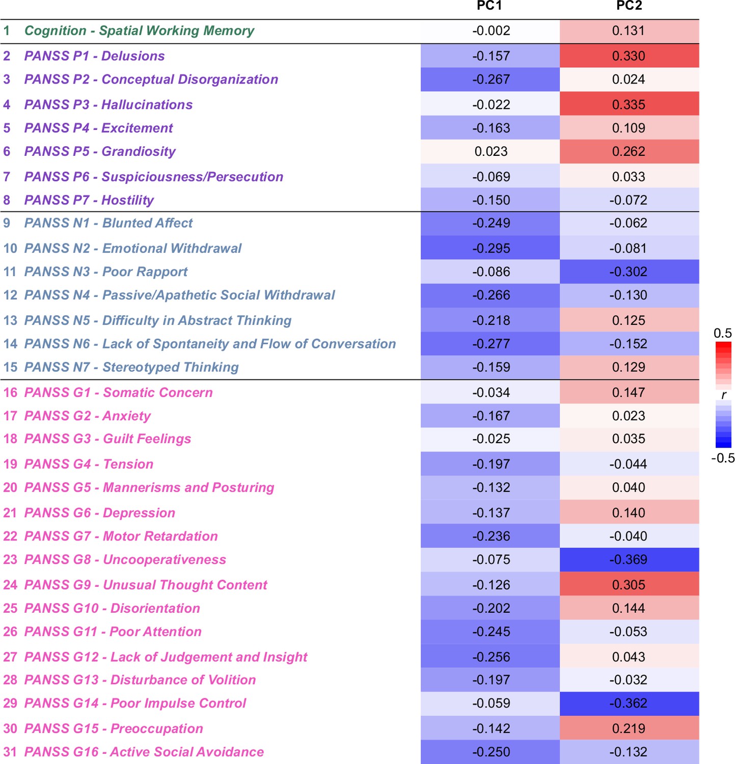
Delta Behavioral Principal Component (PCA) Loadings.
Table of the loadings of each of the 31 behavioral items on the two significant PCs (also seen in radar plot in Figure 4D). Green = cognition, purple = PANSS positive, blue = PANSS negative, pink = PANSS general. Positive loadings are indicated in red; negative loadings are shown in blue.
-
Figure 4—figure supplement 1—source data 1
- https://cdn.elifesciences.org/articles/84173/elife-84173-fig4-figsupp1-data1-v1.pdf
Figure 4—figure supplement 2
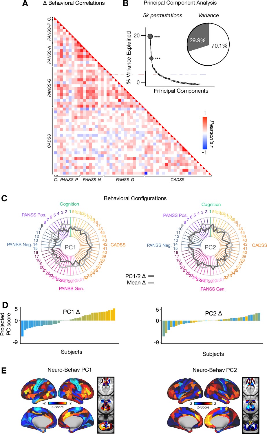
Principal Component Analysis: PANSS, CADSS & Cognition.
(A) Correlations between 54 individual item behavioral measures (PANSS, CADSS, Cognition) for all participants (N=40). Δ (ketamine - placebo) behavioral measures are used. (B) Screeplot showing the % variance explained by each of the principal components (PCs) from a PCA performed using all 54 Δ (ketamine - placebo) behavioral measures across 40 participants. The size of each dark grey point is proportional to the variance explained. The first two PCs (dark grey) survived permutation testing (p<.05, 5000 permutations). Together they capture 29.9% of all symptom variance (inset). (C) Loading profiles shown in dark grey across the 54 behavioral items for PC1 Δ (left) and PC2 (right) Δ. The mean Δ score for each behavioral item is also shown in light grey (scaled to fit the same radar plots). Inner circle = -0.5, middle circle = 0, outer circle = 0.5. (D) Bar plot showing the projected PC score for each individual subject (N=40) for PC1 Δ (left) and PC2 (right) Δ. Bars are color coded according to each subject’s PC1 score ranking. (E) Neuro-behavioral PC1-2 maps showing the relationship between the behavioral PC score for each participant regressed onto the Δ GBC map for each participant (N=40). Values shown in each brain parcel are the Z-scored regression coefficient (behavioral PC score, Δ GBC) across all 40 subjects. Red/orange areas indicate parcels in which there is a positive relationship between GBC and the behavioral PC score, while blue areas indicate parcels in which there is a negative relationship between GBC and the behavioral PC score.
Figure 4—figure supplement 3
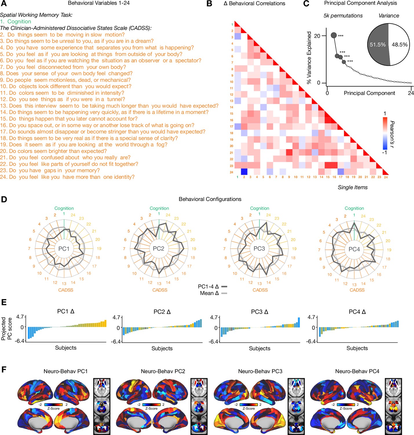
Principal Component Analysis: CADSS & Cognition.
(A) The Clinician-Administered Dissociative States Scale (CADSS) questions. (B) Correlations between 24 individual item behavioral measures (CADSS, Cognition) for all participants (N=40). Δ (ketamine- placebo) behavioral measures are used. (C) Screeplot showing the % variance explained by each of the principal components (PCs) from a PCA performed using all 24 Δ (ketamine - placebo) behavioral measures across 40 participants. The size of each dark grey point is proportional to the variance explained. The first four PCs (dark grey) survived permutation testing (p<.05, 5000 permutations). Together they capture 51.5% of all symptom variance (inset). (D) Loading profiles shown in dark grey across the 24 behavioral items for PC1-4 Δ. The mean Δ score for each behavioral item is also shown in light grey (scaled to fit the same radar plots). Inner circle = -0.5, middle circle = 0, outer circle = 0.5. (E) Bar plot showing the projected PC score for each individual subject (N=40) for PC1-4 Δ. Bars are color coded according to each subject’s PC1 score ranking. (F) Neuro-behavioral PC1-4 maps showing the relationship between the behavioral PC score for each participant regressed onto the Δ GBC mapfor each participant (N=40). Values shown in each brain parcel are the Z-scored regression coefficient (behavioral PC score, Δ GBC) across all 40 subjects. Red/orange areas indicate parcels in which there is a positive relationship between GBC and the behavioral PC score, while blue areas indicate parcels in which there is a negative relationship between GBC and the behavioral PC score.
Figure 5 with 8 supplements
Lower-dimensional behavioral variation reveals robust neuro-behavioral mapping.
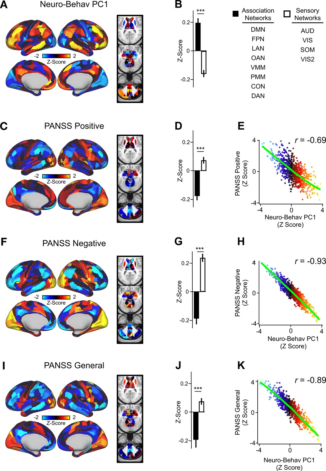
(A) Neuro-behavioral PC1 map showing the relationship between the behavioral PC1 score for each participant regressed onto the Δ GBC map for each participant (N=40). Values shown in each brain parcel are the Z-scored regression coefficient (behavioral PC1 score, Δ GBC) across all 40 subjects. Red/orange areas indicate parcels in which there is a positive relationship between GBC and the behavioral PC1 score, while blue areas indicate parcels in which there is a negative relationship between GBC and the behavioral PC1 score. (B) Bar plot showing the mean correlation (Δ GBC, behavioral PC1 score) for association (black) and sensory (white) networks. (C) PANSS Positive map showing the relationship between the PANSS Positive score for each participant regressed onto the Δ GBC map for each participant (N=40). Values shown in each brain parcel are the Z-scored regression coefficient (PANSS Positive score, Δ GBC) across all 40 subjects. (D) Bar plot showing the mean correlation (Δ GBC, PANSS Positive score) for association (black) and sensory (white) networks. (E) Scatter plot showing the relationship across parcels between neuro-behavioral PC1 and PANSS Positive maps (r=0.69, p<0.001, n=718). (F) PANSS Negative map showing the relationship between the PANSS Negative score for each participant regressed onto the Δ GBC map for each participant (N=40). Values shown in each brain parcel are the Z-scored regression coefficient (PANSS Negative score, Δ GBC) across all 40 subjects. (G) Bar plot showing the mean correlation (Δ GBC, PANSS Negative score) for association (black) and sensory (white) networks. (H) Scatter plot showing the relationship across parcels between neuro-behavioral PC1 and PANSS Negative maps (r=0.93, p<0.001, n=718). (I) PANSS General map showing the relationship between the PANSS General score for each participant regressed onto the Δ GBC map for each participant (N=40). Values shown in each brain parcel are the Z-scored regression coefficient (PANSS General score, Δ GBC) across all 40 subjects. (J) Bar plot showing the mean correlation (Δ GBC, PANSS General score) for association (black) and sensory (white) networks. (K) Scatter plot showing the relationship across parcels between neuro-behavioral PC1 and PANSS General maps (r=0.89, p<0.001, n=718). (DMN = default mode, FPN = frontoparietal, LAN = language, OAN = orbito-affective, VMM = ventro multimodal, PMM = posterior multimodal, CON = cingulo-opercular, DAN = dorsal attention, AUD = auditory, VIS = primary visual, SOM = somatomotor, VIS2=secondary visual).
Figure 5—figure supplement 1

Comparison of three principal component analyses: 1. PANSS & Cognition; 2. PANSS, CADSS, & Cognition;and 3. CADSS, & Cognition.
(A-B) Neuro-behavioral PC1-2 maps from the PCA conducted on PANSS & Cognition data. Maps show the relationship between the behavioral PC score for each participant regressed onto the Δ GBC map for each participant (N=40). Values shown in each brain parcel are the Z-scored regression coefficient (behavioral PC score, Δ GBC) across all 40 subjects. Red/orange areas indicate parcels in which there is a positive relationship between GBC and the behavioral PC score, while blue areas indicate parcels in which there is a negative relationship between GBC and the behavioral PC score. (C) Correlation between the resulting neuro-behavioral PC maps from a principal component analysis conducted on either: 1. PANSS and Cognition data (i.e. PANSS PC1-2); 2. CADSS, & Cognition data (i.e. CADSS PC1-4) ; or 3. PANSS, CADSS, and Cognition data (i.e. PANSS and CADSS PC1-2). (D-E) Neuro-behavioral PC1-2 maps from the PCA conducted on CADSS & Cognition data. Maps show the relationship between the behavioral PC score for each participant regressed onto the Δ GBC map for each participant (N=40). Values shown in each brain parcel are the Z-scored regression coefficient (behavioral PC score, Δ GBC) across all 40 subjects. (F-I) Neuro-behavioral PC1-4 maps from the PCA conducted on PANSS, CADSS, and Cognition data. Maps show the relationship between the behavioral PC score for each participant regressed onto the Δ GBC map for each participant (N=40). Values shown in each brain parcel are the Z-scored regression coefficient (behavioral PC score, Δ GBC) across all 40 subjects.
Figure 5—figure supplement 2

Correlations between PC1-5 Δ GBC, neuro-behavioral PC1-2, and mean Δ GBC maps.
The PC1 Δ GBC mapis highly negatively correlated with the neuro-behavioral PC1 map (r=-0.62) and the mean Δ GBC map (r=-0.56), while neural-behavioral PC2 map is moderately positively correlated with the mean Δ GBC map (r=0.41). * = p<.05, ** = p<.01, *** = p<.001.
Figure 5—figure supplement 3

Neuro-behavioral PC1, PANSS negative, and PANSS general track SST and PVALB gene expression to-pographies.
(A) Neuro-behavioral PC1 map showing the relationship between the behavioral PC1 score for each participant regressed onto the Δ GBC map for each participant (N=40). (B) Bar plot showing the correlation between the neuro-behavioral PC1 map and the following gene expression maps: SST (r=0.29, p=.009) (red) and PVALB (r=-0.14, p=.089) (blue). All p-values are FDR corrected. (C) Distribution of 100,000 simulated r values for neuro-behavioral PC1 and: SST (bottom), PVALB (top). Bold lines indicate the observed r value between neuro-behavioral PC1 and: SST (red), PVALB (blue). (D) Neuro-behavioral PC2 map showing the relationship between the behavioral PC2 score for each participant regressed on to the GBC map for each participant. (E) Bar plot showing the correlation between the neuro-behavioral PC2 map and the following gene Δ expression maps: SST (r=0.09, p=.22) (red) and PVALB (r=0.01, p=.75) (blue). All p-values are FDR corrected. (F) Distribution of 100,000 simulated r values for neuro-behavioral PC2 and: SST (bottom), PVALB (top). Bold lines indicate the observed r value between PANSS negative and: SST (red), PVALB (blue). (G) PANSS positive map showing the relationship between the PANSS positive score for each participant regressed onto the GBC Δ map for each participant. (H) Bar plot showing the correlation between the PANSS positive map and the following gene expression maps: SST (r=-0.19, p=.103) (red) and PVALB (r=0.12, p=.164) (blue). All p-values are FDR corrected. (I) Distribution of 100,000 simulated r values for PANSS positive and: SST (bottom), PVALB (top). Bold lines indicate the observed r value between PANSS positive and: SST (red), PVALB (blue). (J) PANSS negative map showing the relationship between the PANSS negative score for each participant regressed onto the Δ GBC map for each participant. (K) Bar plot showing the correlation between the PANSS negative map and the following gene expression maps: SST (r=-0.34, p<.001) (red) and PVALB (r=0.16, p=.05) (blue). All p-values are FDR corrected. (L) Distribution of 100,000 simulated r values for PANSS negative and: SST (bottom), PVALB (top). Bold lines indicate the observed r value between PANSS negative and: SST (red), PVALB (blue). (M) PANSS general map showing the relationship between the PANSS general score for each participant regressed onto the Δ GBC map for each participant. (N) Bar plot showing the correlation between the PANSS general map and the following gene expression maps: SST (r=-0.26, p=.019) (red) and PVALB (r=0.18, p=.04) (blue).All p-values are FDR corrected. (O) Distribution of 100,000 simulated r values for PANSS general and: SST (bottom), PVALB (top). Bold lines indicate the observed r value between PANSS general and: SST (red), PVALB (blue). (P) Cognition map showing the relationship between the cognition score for each participant regressed onto the Δ GBC map for each participant. (Q) Bar plot showing the correlation between the cognition map and the following gene expression maps: SST (r=0.03, p=.84) (red) and PVALB (r=0.09, p=.33) (blue). All p-values are FDR corrected. (R) Distribution of 100,000 simulated r values for cognition and: SST (bottom), PVALB (top). Bold lines indicate the observed r value between cognition and: SST(red), PVALB (blue).
Figure 5—figure supplement 4
Network breakdown of neuro-behavioral PC1 and neuro-behavioral PC2.
(A) Neuro-behavioral PC1 map showing the relationship between the behavioral PC1 score for each participant regressed onto the Δ GBC map for each participant (N=40). Values shown in each brain parcel are the Z-scored regression coefficient (behavioral PC1 score, Δ GBC) across all 40 subjects. Red/orange areas indicate parcels in which there is a positive relationship between GBC and the behavioral PC1 score, while blue areas indicate parcels in which there is a negative relationship between GBC and the behavioral PC1 score. (B) Bar plot showing the neuro-behavioral PC1 GBC Z-score across association (black) and sensory (white) network parcels. (C) Bar plot showing the mean correlation (Δ GBC, behavioral PC1 score) for each network and each anatomical subcortical structure (see inset right for color labels). (D) Neuro-behavioral PC2 map showing the relationship between the behavioral PC2 score for each participant regressed onto the Δ GBC map for each participant (N=40). Values shown in each brain parcel are the Z-scored regression coefficient (behavioral PC2 score, Δ GBC) across all 40 subjects. Red/orange areas indicate parcels in which there is a positive relationship between GBC and the behavioral PC2 score, while blue areas indicate parcels in which there is a negative relationship between GBC and the behavioral PC2 score. (E) Bar plot showing the neuro-behavioral PC2 GBC Z-score across association (black) and sensory (white) network parcels. (F) Bar plot showing the mean correlation (Δ GBC, behavioral PC2 score) for each network and each anatomical subcortical structure (see inset right for color labels).
Figure 5—figure supplement 5

Network breakdown of existing behavioral measures: 3-factor PANSS subscales and cognition Δ GBC maps.
(A) PANSS positive map showing the relationship between the PANSS positive score for each participant regressed onto the Δ GBC mapfor each participant (N=40). Values shown in each brain parcel are the Z-scored regression coefficient (PANSS positive, Δ GBC) across all 40 subjects. Red/orange areas indicate parcels in which there is a positive relationship between GBC and the PANSS positive score, while blue areas indicate parcels in which there is a negative relationship between GBC and the PANSS positive score. (B) Bar plot showing the mean correlation (Δ GBC, PANSS positive score) for each network and each anatomical subcortical structure (see inset right for color labels). (C) PANSS negative map showing the relationship between the PANSS negative score for each participant regressed onto the Δ GBC map for each participant (N=40).Values shown in each brain parcel are the Z-scored regression coefficient (PANSS negative, Δ GBC) across all 40 subjects. Red/orange areas indicate parcels in which there is a positive relationship between GBC and the PANSS negative score, while blue areas indicate parcels in which there is a negative relationship between GBC and the PANSS negative score. (D) Bar plot showing the mean correlation (Δ GBC, PANSS negative score) for each network and each anatomical subcortical structure (see inset right for color labels). (E) PANSS general map showing the relationship between the PANSS general score for each participant regressed onto the Δ GBC map for each participant (N=40). Values shown in each brain parcel are the Z-scored regression coefficient (PANSS general, Δ GBC) across all 40 subjects. Red/orange areas indicate parcels in which there is a positive relationship between GBC and the PANSS general score, while blue areas indicate parcels in which there is a negative relationship between GBC and the PANSS general score. (F) Bar plot showing the mean correlation (Δ GBC, PANSS general score) for each network and each anatomical subcortical structure (see inset right for color labels). (G) Cognition map showing the relationship between the cognition score for each participant regressed onto the Δ GBC map for each participant (N=40). Values shown in each brain parcel are the Z-scored regression coefficient (cognition, Δ GBC) across all 40 subjects. Red/orange areas indicate parcels in which there is a general relationship between GBC and the cognition score,while blue areas indicate parcels in which there is a negative relationship between GBC and the cognition score. (L) Bar plot showing the mean correlation (Δ GBC, cognition score) for each network and each anatomical subcortical structure (see inset right for color labels).
Figure 5—figure supplement 6
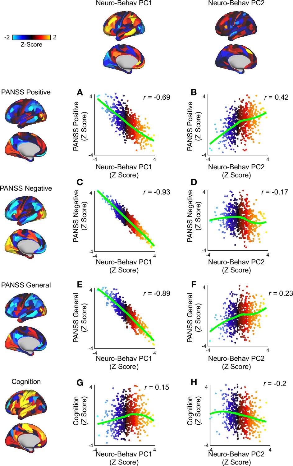
Scatter plots showing the relationship between neuro-behavioral PC1-2 and the 3-factor PANSS subscales.
(A) Scatter plot showing the relationship between PANSS positive (left) and neuro-behavioral PC1 (top). (B) Scatter plot showing the relationship between PANSS positive (left) and neuro-behavioral PC2 (top). (C) Scatter plot showing the relationship between PANSS negative (left) and neuro-behavioral PC1 (top). (D) Scatter plot showing the relationship between PANSS negative (left) and neuro-behavioral PC2 (top). (E) Scatter plot showing the relationship between PANSS general (left) and neuro-behavioral PC1 (top). (F) Scatter plot showing the relationship between PANSS general (left) and neuro-behavioral PC2 (top). (G) Scatter plot showing the relationship between cognition (left) and neuro-behavioral PC1 (top)(r=0.15, p). (H) Scatter plot showing the relationship between cognition (left) and neuro-behavioral PC2 (top).
Figure 5—figure supplement 7
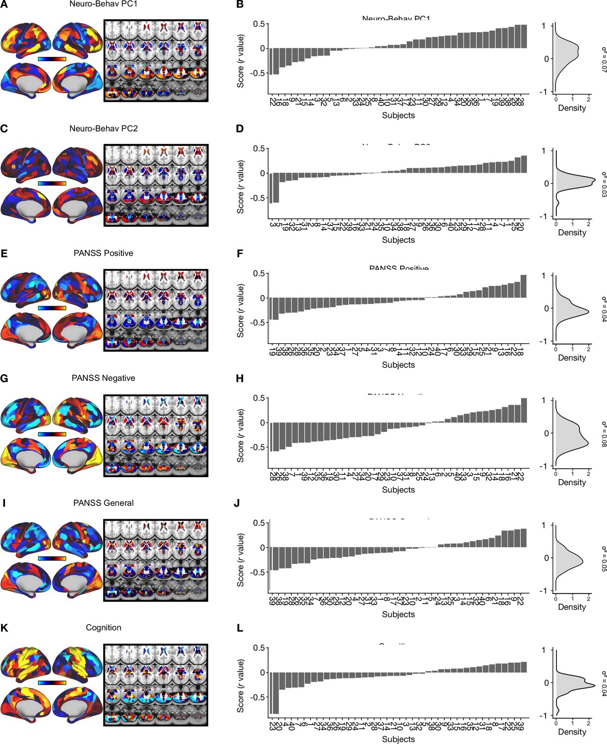
Individual variation captured by neuro-behavioral PCs, 3-factor PANSS subscales, and cognition Δ GBCmaps.
(A) Neuro-behavioral PC1 map showing the relationship between the behavioral PC1 score for each participant regressed onto the Δ GBC map for each participant (N=40). (B) (Left) Bar plot showing the neuro-behavioral PC1 score (r) for each participant (N=40). Neuro-behavioral PC1scores were calculated by correlating each participant’s individual Δ GBC map with the neuro-behavioral PC1 Δ GBC map. (Right) density plot of neuro-behavioral PC1 scores. (C) Neuro-behavioral PC2 map showing the relationship between the behavioral PC2 score for each participant regressed onto the Δ GBC map for each participant. (D) (Left) Bar plot showing the neuro-behavioral PC2 score (r) for each participant (N=40). Neuro-behavioral PC2 scores were calculated by correlating each participant’s individual Δ GBC map with the neuro-behavioral PC2 Δ GBC map. (Right) density plot of neuro-behavioral PC2 scores. (E) PANSS positive map showing the relationship between the PANSS positive score for each participant regressed onto the Δ GBC map for each participant. (F) (Left) Bar plot showing the PANSS positive score (r) for each participant (N=40). PANSS positive scores were calculated by correlating each participant’s individual Δ GBC map with the PANSS positive Δ GBC map. (Right) density plot of PANSS positive scores. (G) PANSS negative map showing the relationship between the PANSS negative score for each participant regressed on to the Δ GBC map for each participant. (H) (Left) Bar plot showing the PANSS negative score (r) for each participant (N=40). PANSS negative scores were calculated by correlating each participant’s individual Δ GBC map with the PANSS negative Δ GBC map. (Right) density plot of PANSSnegative scores. (I) PANSS general map showing the relationship between the PANSS general score for each participant regressed onto the Δ GBCmap for each participant. (J) (Left) Bar plot showing the PANSS general score (r) for each participant (N=40). PANSS general scores were calculated by correlating each participant’s individual Δ GBC map with the PANSS general Δ GBC map. (Right) density plot of PANSS general scores. (K) Cognition map showing the relationship between the cognition score for each participant regressed onto the Δ GBC map for each participant. (L) (Left) Bar plot showing the cognition score (r) for each participant (N=40). Cognition scores were calculated by correlating each participant’s individual Δ GBC map with the cognition Δ GBC map. (Right) density plot of cognition scores.
Figure 5—figure supplement 8
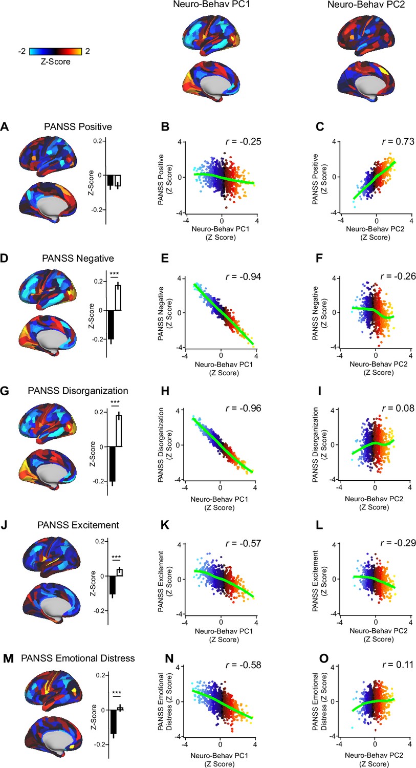
Scatter plots showing the relationship between neuro-behavioral PC1-2 and the 5-factor PANSS subscales.
(A, D, G, J, M) (left) Maps showing the relationship between the 5-factor PANSS subscale score for each participant regressed onto the Δ GBC map for each participant (N=40). Values shown in each brain parcel are the Z-scored regression coefficient (PANSS subscale, Δ GBC) across all 40 subjects. Red/orange areas indicate parcels in which there is a positive relationship between GBC and the PANSS subscale score, while blue areas indicate parcels in which there is a negative relationship between GBC and the PANSS subscale score. (right) Bar plot showing the mean Z-scored correlation value (PANSS subscale, Δ GBC) for association (black) and sensory (white) networks. (B) Scatter plot showing the relationship between PANSS positive (left) and neuro-behavioral PC1 (top). (C) Scatter plot showing the relationship between PANSS positive (left) and neuro-behavioral PC2 (top). (E) Scatter plot showing the relationship between PANSS negative (left) and neuro-behavioral PC1 (top). (F) Scatter plot showing the relationship between PANSS negative (left) and neuro-behavioral PC2 (top). (H) Scatter plot showing the relationship between PANSS disorganization (left) and neuro-behavioral PC1 (top). (I) Scatter plot showing the relationship between PANSS disorganization (left) and neuro-behavioral PC2 (top). (K) Scatter plot showing the relationship between PANSS excitement (left) and neuro-behavioral PC1 (top). (L) Scatter plot showing the relationship between PANSS excitement (left) and neuro-behavioral PC2 (top). (N) Scatter plot showing the relationship between PANSS emotional distress (left) and neuro-behavioral PC1 (top). (O) Scatter plot showing the relationship between PANSS emotional distress (left) and neuro-behavioral PC2 (top).
Figure 6 with 4 supplements
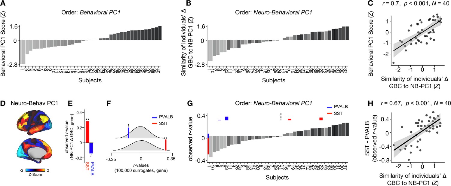
Individual variation in ketamine-induced neuro-behavioral changes.
(A) Bar plot showing the behavioral PC1 score (Z) for each individual participant (N=40). Bars are numbered and color-coded according to each participant’s behavioral PC1 score (light gray = highly negative score, dark gray = highly positive score). (B) Bar plot showing the neuro-behavioral PC1 score (Z) for each individual participant (N=40). The neuro-behavioral PC1 score is calculated by correlating each participant’s Δ GBC map with the neuro-behavioral PC1 map, and then Z-scoring the r-values. Bars are ordered according to each participant’s neuro-behavioral PC1 score, but labelled and color-coded according to each participant’s behavioral PC1 score (light gray = h ighly negative score, dark gray = highly positive score). (C) Correlation between each participant’s behavioral PC1 score and their neuro-behavioral PC1 score (r=0.7, p<0.001). (D) Neuro-behavioral PC1 map showing the relationship between the behavioral PC1 score for each participant regressed onto the Δ GBC map for each participant (N=40). (E) Bar plot showing the correlation between the neuro-behavioral PC1 map and the following gene expression maps: SST (r=0.29, p=0.009) (red) and PVALB (r=−0.14, p=0.089) (blue). All p-values are FDR corrected. (F) Distribution of 100,000 simulated r values for neuro-behavioral PC1 and: SST (bottom), PVALB (top). Bold lines indicate the observed r value between neuro-behavioral PC1 and: SST (red), PVALB (blue). (G) Bar plot showing the relationship between SST (red) and PVALB (blue) gene expression maps and each participants Δ GBC maps (i.e. the observed r-value). Participants are ordered according to their neuro-behavioral PC1 score (i.e. the similarity between their Δ GBC map and the neuro-behavioral PC1 map). Subjects to the left of the dashed line load negatively onto neuro-behavioral PC1, while subjects to the right of the dashed line load positively onto neuro-behavioral PC1. (H) Correlation between the difference (SST - PVALB) in observed r values for each participant, and their neuro-behavioral PC1 score (r=0.67, p<0.001).
Figure 6—figure supplement 1
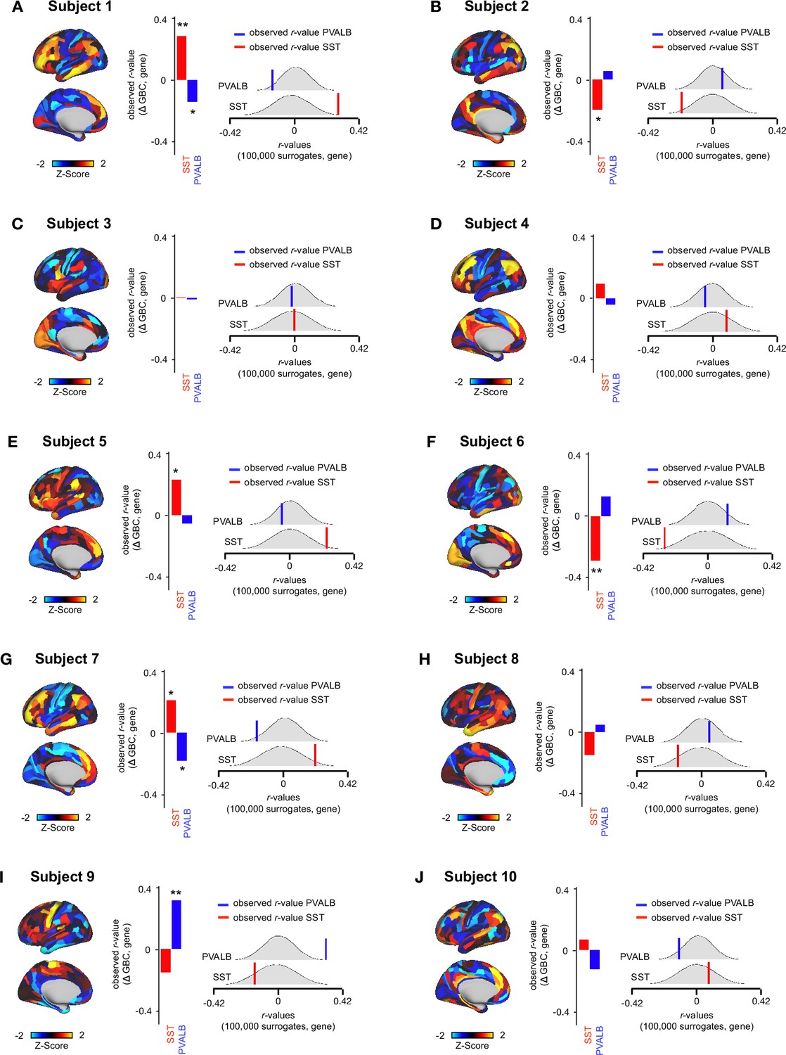
Relationship between Δ GBC maps and SST/PVALB gene expression maps for subjects 1-10.
(A-J) (left) Unthresholded Δ GBC Z-score maps (Z-scores computed across 718 parcels) for subjects 1-10. Red/orange areas indicate parcels that show increased GBC following ketamine, while blue areas indicate parcels that show decreased GBC following ketamine. (centre) Bar plots showing the correlation between the Δ GBC map and SST (red) and PVALB (blue) gene expression maps for subjects 1-10. (right) Distribution of 100,000 simulated r values for SST (bottom) and PVALB (top). Bold lines indicate the observed r value between each subject’s Δ GBC and SST (red) and PVALB (blue) gene expression maps.
Figure 6—figure supplement 2

Relationship between Δ GBC maps and SST/PVALB gene expression maps for subjects 11-20.
(A-J) (left) Unthresholded Δ GBC Z-score maps (Z-scores computed across 718 parcels) for subjects 11-20. Red/orange areas indicate parcels that show increased GBC following ketamine, while blue areas indicate parcels that show decreased GBC following ketamine. (centre) Bar plots showing the correlation between the Δ GBC map and SST (red) and PVALB (blue) gene expression maps for subjects 11-21. (right) Distribution of 100,000 simulated r values for SST (bottom) and PVALB (top). Bold lines indicate the observed r value between each subject’s Δ GBC and SST (red) and PVALB (blue) gene expression maps.
Figure 6—figure supplement 3
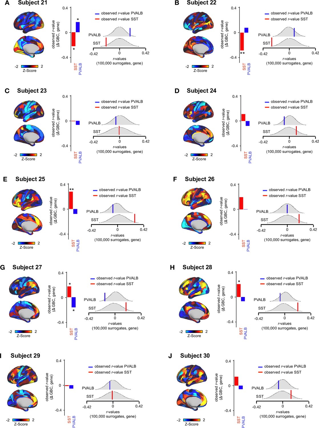
Relationship between Δ GBC maps and SST/PVALB gene expression maps for subjects 21-30.
(A-J) (left) Unthresholded Δ GBC Z-score maps (Z-scores computed across 718 parcels) for subjects 21-30. Red/orange areas indicate parcels that show increased GBC following ketamine, while blue areas indicate parcels that show decreased GBC following ketamine. (centre) Bar plots showing the correlation between the Δ GBC map and SST (red) and PVALB (blue) gene expression maps for subjects 21-30. (right) Distribution of 100,000 simulated r values for SST (bottom) and PVALB (top). Bold lines indicate the observed r value between each subject’s Δ GBC and SST (red) and PVALB (blue) gene expression maps.
Figure 6—figure supplement 4

Relationship between Δ GBC maps and SST/PVALB gene expression maps for subjects 31-40.
(A-J) (left) Unthresholded Δ GBC Z-score maps (Z-scores computed across 718 parcels) for subjects 31-40. Red/orange areas indicate parcels that show increased GBC following ketamine, while blue areas indicate parcels that show decreased GBC following ketamine. (centre) Bar plots showing the correlation between the Δ GBC map and SST (red) and PVALB (blue) gene expression maps for subjects 31-40. (right) Distribution of 100,000 simulated r values for SST (bottom) and PVALB (top). Bold lines indicate the observed r value between each subject’s Δ GBC and SST (red) and PVALB (blue) gene expression maps.
Tables
Key resources table
| Reagent type (species) or resource | Designation | Source or reference | Identifiers | Additional information |
|---|---|---|---|---|
| Software, algorithm | QuNex | QuNex, Ji et al., 2023 | ||
| Software, algorithm | HCP MPP | HCP MPP, Glasser et al., 2013 | ||
| Software, algorithm | N-BRIDGE | N-BRIDGE, Ji et al., 2020 | ||
| Software, algorithm | CAB-NP | CAB-NP, Ji et al., 2019 | ||
| Software, algorithm | R | R | RRID:SCR_001905 | |
| Software, algorithm | FSL | FSL | RRID:SCR_002823 |
Additional files
-
Supplementary file 1
Retrospectively assessed (180 mins after drug administration) ketamine-induced subjective effects.
Effects were assessed using the Clinician Administered Dissociative States Scale (CADSS), the Positive and Negative Syndrome Scale for positive symptoms, negative symptoms and general psychopathology, and the Beck’s Depression Inventory (BDI). N=40. ** indicates P<.001
- https://cdn.elifesciences.org/articles/84173/elife-84173-supp1-v1.pdf
-
Supplementary file 2
Demographic Information.
- https://cdn.elifesciences.org/articles/84173/elife-84173-supp2-v1.pdf
-
Supplementary file 3
Difference in PANSS Total for each individual participant following ketamine vs. placebo administration.
For each participant we conducted a paired t-test comparing their PANSS Total score following either ketamine for placbeo administration. * significant at P<.05 uncorrected.
- https://cdn.elifesciences.org/articles/84173/elife-84173-supp3-v1.pdf
-
Supplementary file 4
Number of outliers for each PANSS Item and Cognition Δ (ketamine - placebo) scores.
* these items have an interquartile range of 0 so any scores above or below 0 are defined as outliers. Outlier is defined as <Q1-1.5*IQR/>Q3+1.5*IQR where IQR = interquartile range, Q1=first quartile, and Q3=third quartile.
- https://cdn.elifesciences.org/articles/84173/elife-84173-supp4-v1.pdf
-
MDAR checklist
- https://cdn.elifesciences.org/articles/84173/elife-84173-mdarchecklist1-v1.docx
Download links
A two-part list of links to download the article, or parts of the article, in various formats.
Downloads (link to download the article as PDF)
Open citations (links to open the citations from this article in various online reference manager services)
Cite this article (links to download the citations from this article in formats compatible with various reference manager tools)
Ketamine induces multiple individually distinct whole-brain functional connectivity signatures
eLife 13:e84173.
https://doi.org/10.7554/eLife.84173


