Projection neurons in Drosophila antennal lobes signal the acceleration of odor concentrations
- Columbia University, United States
Figures
Figure 1 with 1 supplement

Dynamics of sample odor stimuli are significantly transformed along an odor-OSN-PN pathway.
(A) An experimental setup. Activity of OSNs and PNs was recorded in two different assays, which share the same odor delivery system. A photoionization detector (PID) provided real-time measurements of odor concentrations in every trial. (B) Sample traces of OSN and PN responses to a triangle-shaped odor concentration profile. (C) Sample OSN and PN responses to five distinct odor concentration waveforms. (Top row) Odor concentration profiles. Each trace is an average of six interleaved trials, recorded in the OSN assay. (Middle row) Raster and peristimulus–time histogram (PSTH) plots of the Or59b OSN response. (Bottom row) Raster and PSTH plots of the postsynaptic DM4 PN response to the same panel of odor stimuli.
Figure 1—figure supplement 1
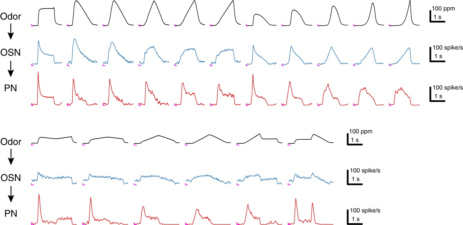
Sample traces of 17 acetone odor concentration waveforms and their responses in Or59b OSNs and DM4 PNs.
Each trace represents an average of 4–6 trials, and the odor concentration was measured in the OSN assay. An ‘L’ mark in magenta at the bottom left corner of each panel represents the zero amplitude point and zero time point for each stimulus epoch.
Figure 2 with 1 supplement
Correlation structures of olfactory information representations in odor, OSN and PN signals.
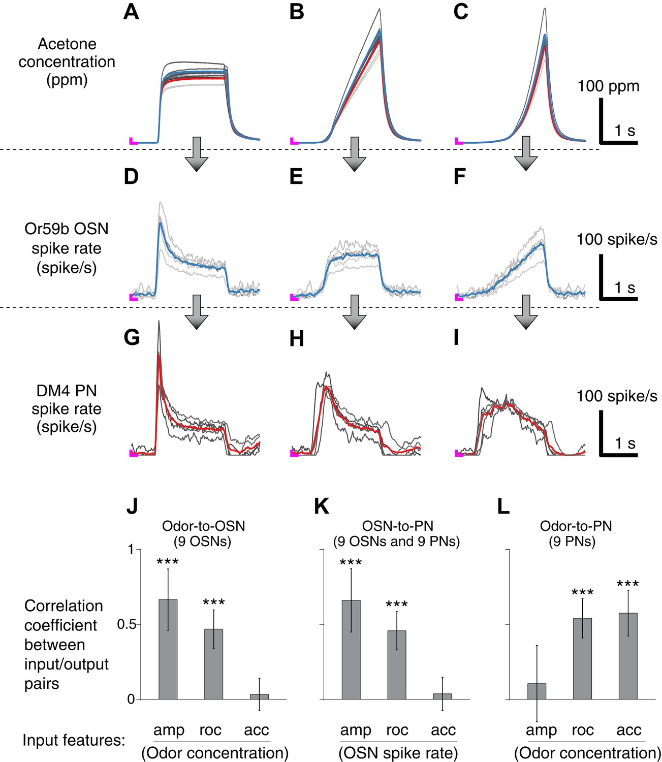
(A–C) Three polynomial odor stimuli: a pulse, a ramp and a parabola. Light gray lines represent individual trials from five different OSN experiments, and dark gray lines represent individual traces from five different PN experiments. Blue and red lines are average traces, respectively, from the OSN and PN experiments. An ‘L’ mark in magenta at the bottom left corner of each panel represents the zero amplitude point. (D–F) Or59b OSN response to the above stimuli (n = 5 flies). (G–I) PN response to the same set of stimuli (n = 5 flies). (J–L) Correlation analyses between three pairs of input and output (amp: amplitude, roc: rate of change, acc: acceleration). OSNs and PNs mainly encode the amplitude and rate of change of their feedforward inputs, whereas PNs most strongly represent the acceleration and rate-of-change components of the odor input. Results with error bars indicate mean ± standard deviation, and ***indicates p < 0.001 (t-test). n = 9 flies for each analysis, 5 flies from the above traces and 4 flies from the same experiment at half concentration (data not shown).
Figure 2—figure supplement 1
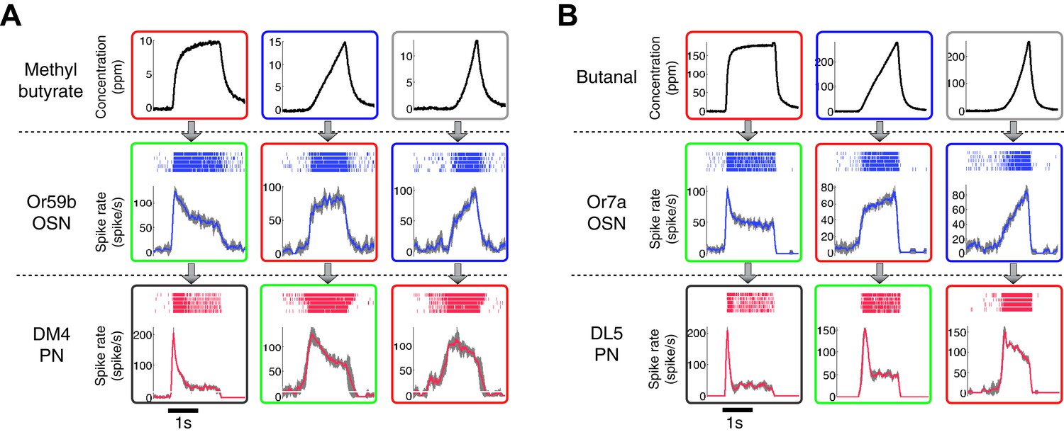
The patterns of the dynamic odor encoding were preserved for different combinations of odorants and OSN-PN pairs.
(A) Outputs of an Or59b OSN and a DM4 PN in response to methyl butyrate polynomial odor inputs. Gray areas represent the standard deviation of the estimated OSN/PN output. (B) Outputs of an Or7a OSN and a DL5 PN in response to butanal polynomial odor inputs. Gray areas represent the standard deviation of the estimated OSN/PN output.
Figure 3 with 1 supplement
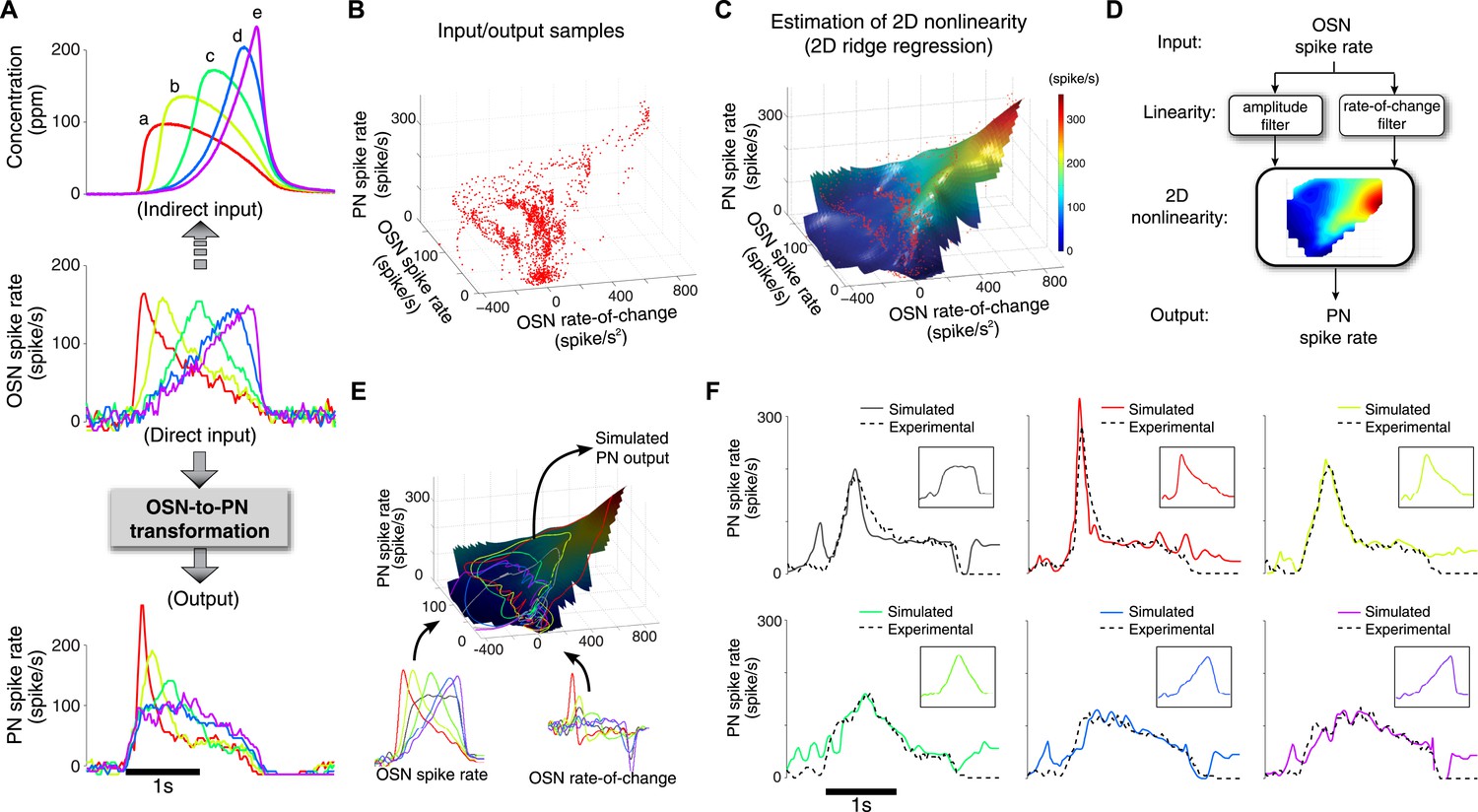
A simple two-dimensional (2D) model characterizes the OSN-to-PN transformation.
(A) Input/output traces used in modeling the OSN-to-PN transformation (n = 5 trials for both OSN and PN data). An ensemble of triangle-shaped OSN spike rates (middle) were designed as a direct in vivo input to the PNs. These OSN spiking patterns were induced by an ensemble of parabola odor inputs (top). (B) Input and output samples for the 2D nonlinearity block. Input axes are OSN spike rate and its rate of change, and the output is the PN spike rate. The samples were estimated from the OSN and PN spike trains with 25-ms sampling interval and depicted as a red dot in the input/output space. (C) A 2D nonlinearity was estimated by ridge regression method from the samples marked in (B). (D) A simple 2D model of the OSN-to-PN transformation, as a 2D linear-nonlinear model. (E) The 2D model was tested for a set of OSN spike rates to evaluate its predictive ability. The black surface depicts a three-dimensional rendering of the 2D nonlinearity in (B). Six OSN spike rates—five triangle-shaped signals and one step-pulse-shaped input—and their rate-of-change functions were projected to the surface. Amplitude readouts from the trajectories on the surface constitute the simulated PN output. The step-pulse-shaped input was introduced for cross-validation of the model since this input was not used for building the model. (F) The predicted PN spike rate closely followed the magnitude and dynamics of the experimental PN spike rate, for six OSN spike rate inputs (insets). The average prediction errors are 31, 26, 21, 21, 23, 29 spike/s (clockwise from the top-left corner, in root-mean-square error).
Figure 3—figure supplement 1
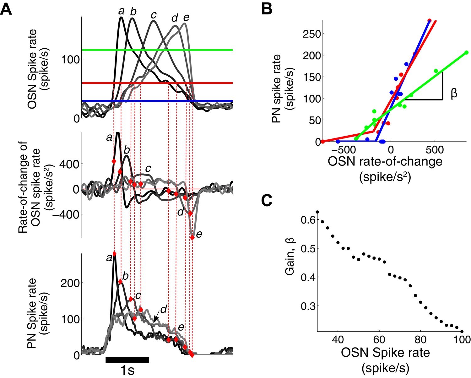
PN output is dependent on both OSN spike rate and its rate of change.
(A) The triangle-shaped OSN spike rate (top), its rate of change (middle), and the corresponding PN spike rates (bottom). At a fixed OSN spike rate (60 spike/s, a solid red line in the top panel), the PN spike rate varies from 0 to 280 spike/s depending on the rate-of-change value of the OSN spike rate. (B) At a fixed OSN spike rate (blue line for 30 spike/s, red line for 60 spike/s, green line for 120 spike/s, as depicted in (A)), the PN spike rate is linearly related to the rate-of-change value of the OSN spike rate with half-wave rectification in the negative rate-of-change interval. (C) The gain β of the PN response, with respect to the rate of change of the OSN output, decreases with increasing input amplitude.
Figure 4
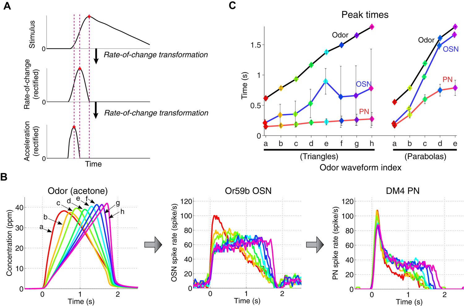
A cascade of rate-of-change encodings leads to a rapid detection of the stimulus onset.
(A) A cascade of two rate-of-change transformations leads to the advancement of the peak time near to the stimulus onset, in response to a triangle-shaped input. At each stage, the rate of change of the input was computed, and the output was half-wave rectified. (B) 8 triangle-shaped acetone concentration waveforms (left) and the corresponding OSN and PN responses. (C) The peak times for odor, OSN, and PN signals. The advancement in peak times was observed in both the odor-to-OSN and OSN-to-PN transformations. Peak times were color coded so that the color of the marker matches that of the associated triangle signals in (B) and parabola signals in Figure 3 (A). n = 5 OSNs and n = 4 PNs for both triangles and parabolas. Results with error bars indicate mean ± standard deviation.
Additional files
-
Source code 1
Custom software written in MATLAB for the analysis of OSN and PN data.
- https://doi.org/10.7554/eLife.06651.010
Download links
A two-part list of links to download the article, or parts of the article, in various formats.
Downloads (link to download the article as PDF)
Open citations (links to open the citations from this article in various online reference manager services)
Cite this article (links to download the citations from this article in formats compatible with various reference manager tools)
Projection neurons in Drosophila antennal lobes signal the acceleration of odor concentrations
eLife 4:e06651.
https://doi.org/10.7554/eLife.06651


