Prediction of primary somatosensory neuron activity during active tactile exploration
- The University of Manchester, United Kingdom
- University of Sussex, United Kingdom
- The Francis Crick Institute, United Kingdom
Figures
Figure 1 with 2 supplements

Electrophysiological recording from single primary whisker units in awake, head-fixed mice and simultaneous measurement of whisker kinematics/mechanics.
(A) Schematic of the preparation, showing a tungsten microelectrode array implanted into the trigeminal ganglion of a head-fixed mouse, whilst a metal pole is presented in one of a range of locations (arrows). Before the start of each trial, the pole was moved to a randomly selected, rostro-caudal location. During this time, the whiskers were out of range of the pole. At the start of the trial, the pole was rapidly raised into the whisker field, leading to whisker-pole touch. Whisker movement and whisker-pole interactions were filmed with a high-speed camera. (B, C) Kinematic (whisker angle θ) and mechanical (whisker curvature κ, moment , axial force ax and lateral force lat) variables were measured for the principal whisker in each video frame. When a whisker pushes against an object during protraction (as in panel D, red and cyan frames), curvature increases; when it pushes against an object during retraction (as in panels B and C), it decreases. (D) Individual video frames during free whisking (yellow and green) and whisker-pole touch (red and cyan) with tracker solutions for the target whisker (the principal whisker for the recorded unit, panel E) superimposed (coloured curve segments). (E) Time series of whisker angle, push angle and curvature change, together with simultaneously recorded spikes (black dots) and periods of whisker-pole contact (red bars). Coloured dots indicate times of correspondingly coloured frames in D.
Figure 1—figure supplement 1
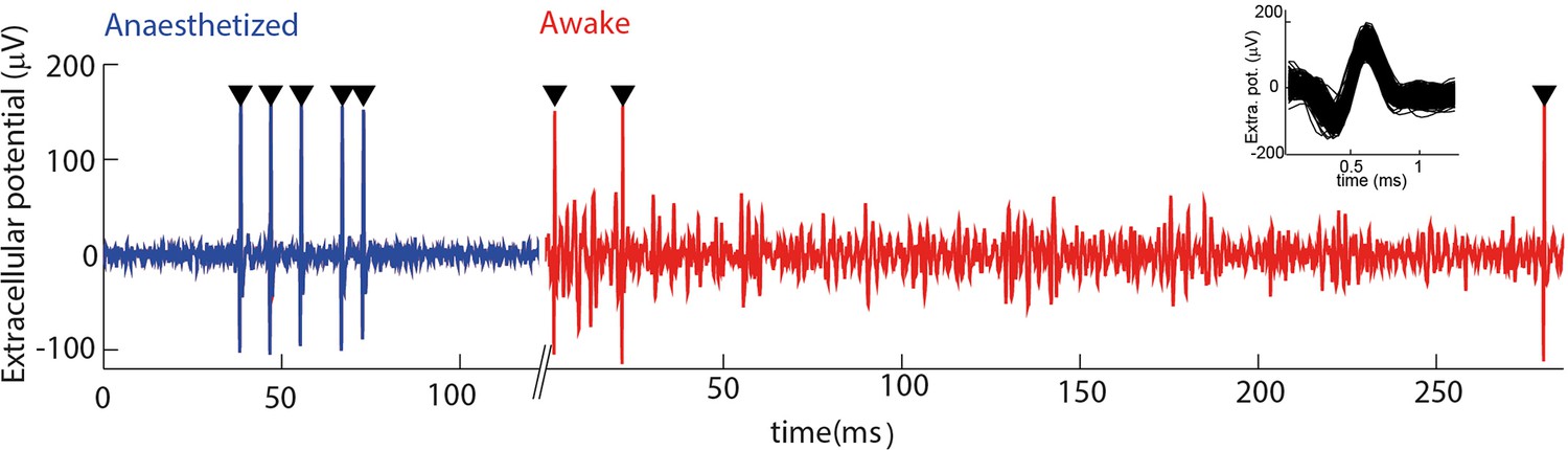
Electrophysiological recording from trigeminal primary neurons of awake, head-fixed mice.
Extracellular potential recorded from the same single unit during both anaesthetized and awake epochs. Spikes belonging to the cluster of the target unit are shown by black triangles. Inset shows overlay of all waveforms belonging to this cluster.
Figure 1—figure supplement 2
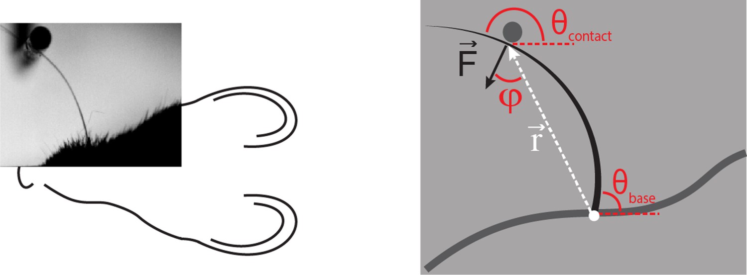
Computation of axial and lateral contact forces.
Axial () and lateral () force components at the whisker base were calculated, in each video frame where there were whisker-pole contacts, as follows (Pammer et al., 2013). First, the point of whisker-pole contact was located (Materials and methods). The direction of the force was then calculated as the normal to the whisker tangent at the contact point (Pammer et al., 2013). Moment at the base M was calculated from the whisker curvature at the base (Materials and methods) and then the magnitude F of was derived from the definition of moment:
where r is the magnitude of the lever arm vector from whisker base to contact point, and φ is the angle between and . The components Fax and Flat were then found by projecting onto the tangent and normal to the whisker at its base, respectively:
,
Here is the angle between the tangent to the whisker at its base and the horizontal; is the angle between and the horizontal.
Figure 2 with 3 supplements
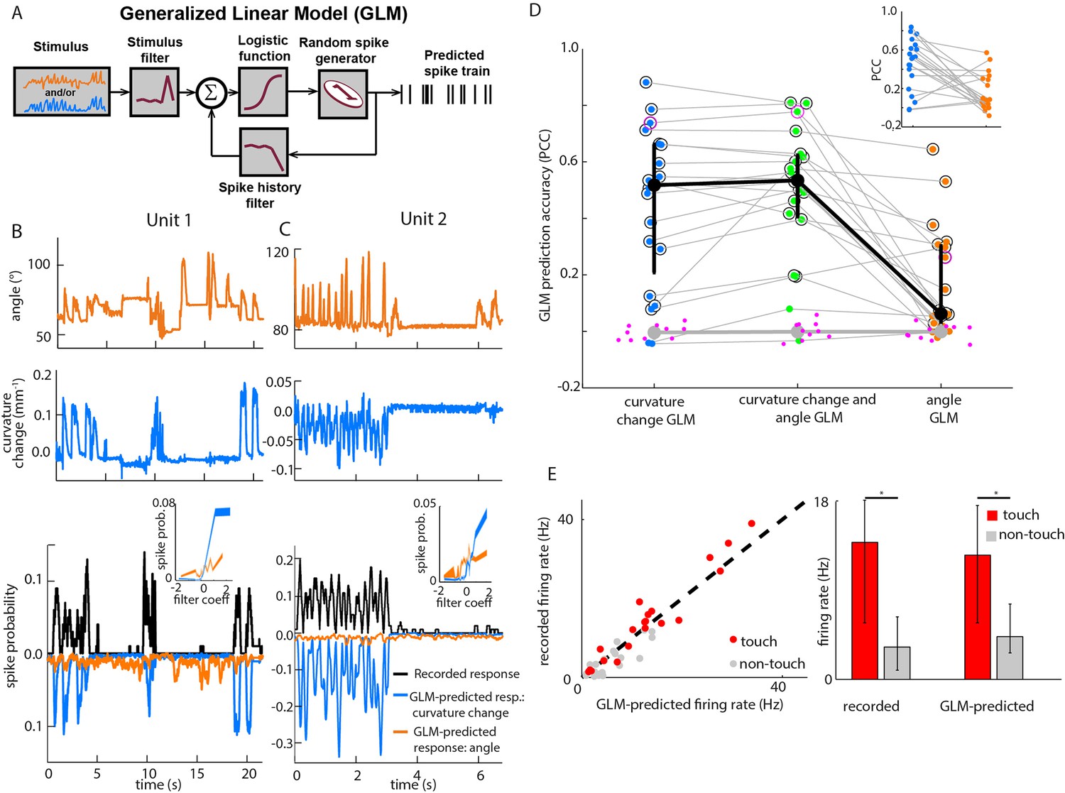
Primary whisker neurons encode whisker curvature, not whisker angle, during active sensation.
(A) Schematic of the Generalized Linear Model (GLM). (B) For an example unit, whisker angle (top panel), whisker curvature change (middle panel) and simultaneously recorded spike train (bottom panel, black), together with predicted spike trains for the best-fitting angle GLM (bottom panel, orange) and curvature change GLM (bottom panel, blue). Spike trains discretized using 1-ms bins and smoothed with a 100 ms boxcar filter. Prediction performance (Pearson correlation coefficient, PCC) for this unit was 0.59. Inset shows tuning curves for both GLMs, computed by convolving the relevant sensory time series (angle or curvature change) with the corresponding GLM stimulus filter to produce a time series of filter coefficients, and estimating the spiking probability as a function of filter coefficient (25 bins). (C) Analogous to panel B, for a second example unit. Prediction performance PCC for this unit was 0.74. (D) Prediction performance (PCC between predicted and recorded spike trains) compared for GLMs fitted with three different types of input: curvature change alone; angle alone; both curvature change and angle. Each blue/orange/green dot is the corresponding PCC for one unit: large black dots indicate median; error bars denote inter-quartile range (IQR). To test statistical significance of each unit’s PCC, the GLM fitting procedure was repeated 10 times on spike trains subjected each time to a random time shift: magenta dots show these chance PCCs for the unit indicated by the magenta circle; the mean chance PCC was computed for each unit and the large grey dot shows the median across units. Black circles indicate units whose PCC was significantly different to chance (signed-rank test, Bonferroni-corrected, p<0.0025). To facilitate direct comparison between results for curvature change GLM and angle GLM, these are re-plotted in the inset. (E) Left. Firing rate during touch episodes compared to that during non-touch episodes for each unit, compared to corresponding predicted firing rates from each unit’s curvature change GLM. Right. Medians across units: error bars denote IQR; * denotes differences significant at p<0.05 (signed-rank test).
Figure 2—figure supplement 1
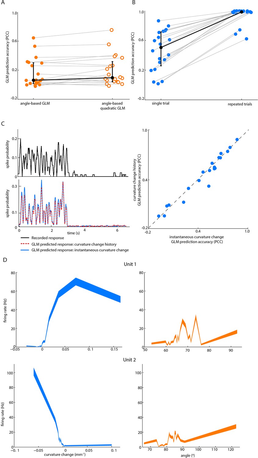
Effect on GLM performance of quadratic input terms, simulated repeated trials and minimal stimulus filters.
(A) Angle GLM prediction performance is robust to addition of quadratic stimulus-dependence. Prediction accuracy (PCC) for standard angle GLM (same data as Figure 2D of main text) in comparison to quadratic GLM (see Materials and methods). Black dots denote medians, error bars IQR. (B) Single-trial GLM prediction accuracy is limited by neuronal response variability. Prediction accuracy (PCC) for simulated neurons. Each simulated neuron is the best-fitting GLM, based on instantaneous curvature change, for its corresponding recorded unit (see Materials and methods). Prediction accuracy is quantified both using the single-trial approach of the main text and using a repeated-trial method only possible by virtue of using a simulation. Black dots denote medians, error bars IQR. (C) Prediction accuracy of curvature-based GLMs is accounted for by tuning to instantaneous curvature change. A GLM performs a temporal filtering operation on its sensory stimulus input and the sensory feature(s) which it encodes is determined by this ‘stimulus filter’. The stimulus filters can, in principle, be complex, but we found that the ability of a GLM to predict spikes (lower left) from curvature change was fully explained by the simple case where the action of the stimulus filter is simply to multiply the sensory input by a gain factor (median 0.55, IQR 0.26–0.66; p=0.35 signed-rank test). Recorded spike train (upper left) and curvature-predicted spike trains (lower left) both for a ‘curvature history’ GLM with a length 5 stimulus filter, as used in Figure 2D of main text, and for an ‘instantaneous curvature’ GLM with a length 1 stimulus filter. Data for unit 2 of main text Figure 2C. Prediction accuracy of the curvature history GLM compared to that of the instantaneous curvature GLM for every recorded unit (right). (D) Tuning curves for curvature change (blue) and angle (orange) of unit 1 and unit 2 in Figure 2.
Figure 2—figure supplement 2
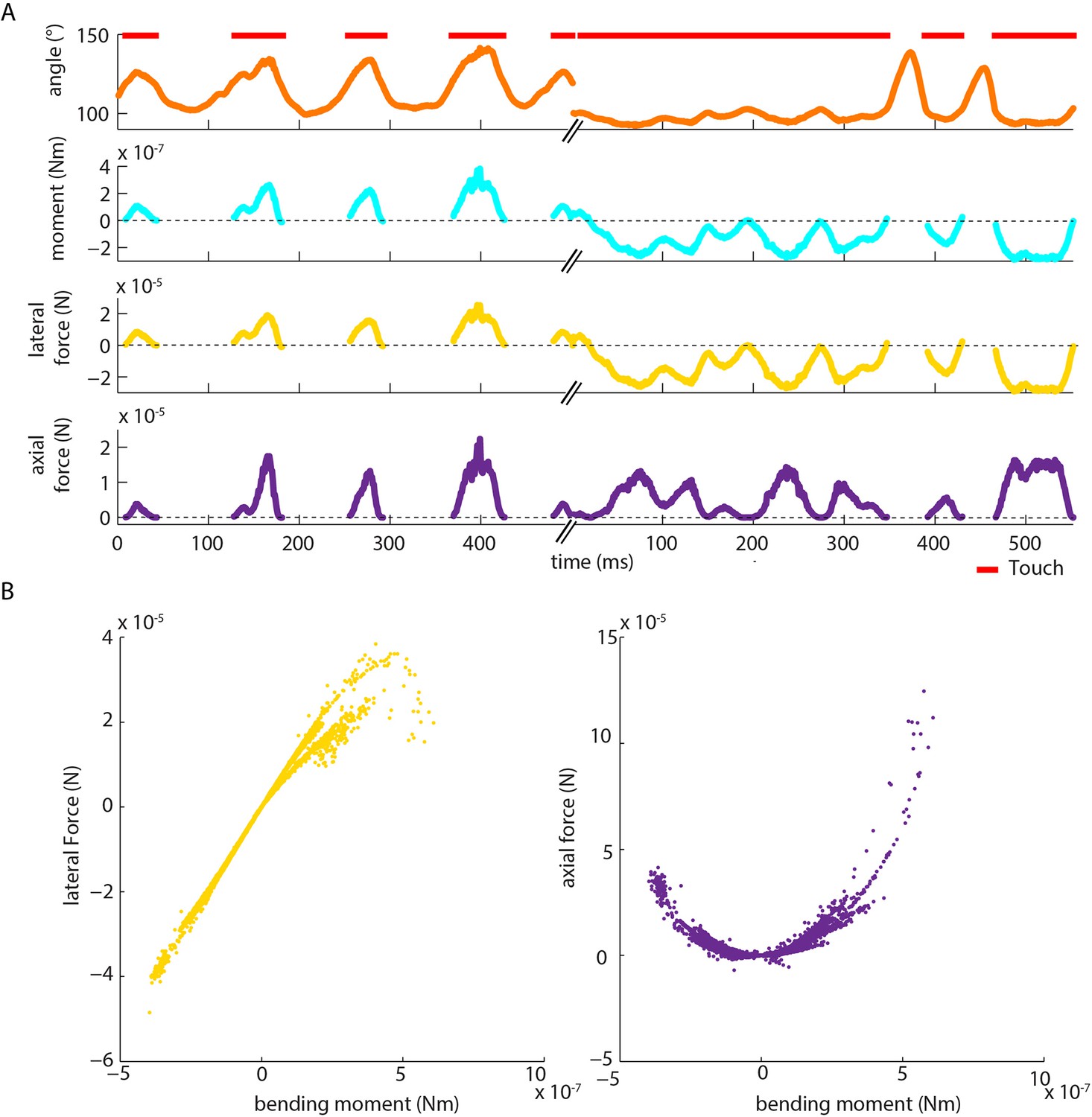
Moment is near-perfectly correlated with axial/lateral contact force components during pole exploration.
(A) Two example time series for simultaneously measured whisker angle, bending moment, lateral force and axial force (see Materials and methods). Red bars indicate episodes of whisker-pole contact. (B) Joint distribution of bending moment and lateral force (left), compared to that of bending moment and axial force (right), for the same recording shown in A. Moment was highly linearly correlated with lateral force (median absolute correlation coefficient across units 0.995, IQR 0.99–1.00, median R2 of linear fit 0.99, IQR 0.97–1.00), and highly quadratically correlated with axial force (median R2 of quadratic fit 0.94, IQR 0.85–0.98). This indicates that, during our conditions of pole exploration, axial force and lateral force are both redundant with moment.
Figure 2—figure supplement 3
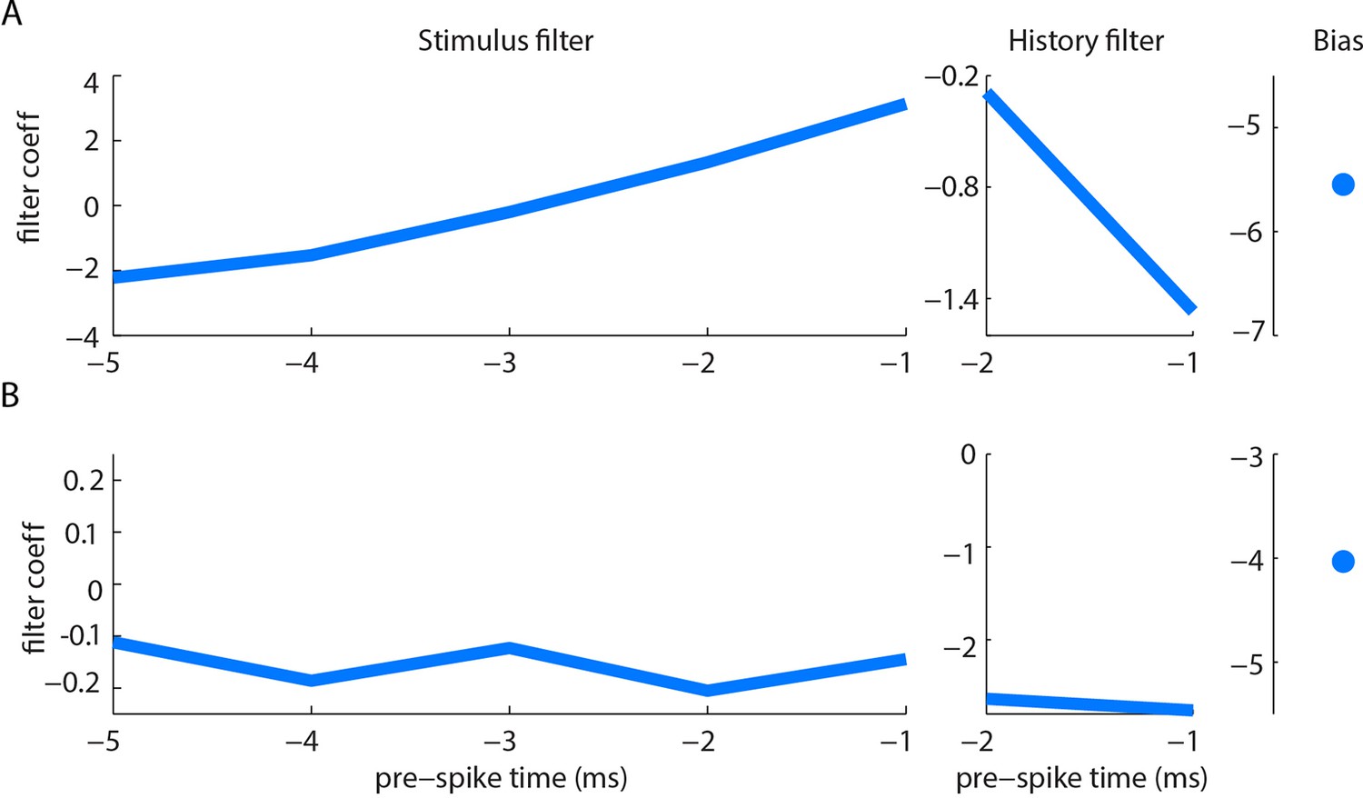
Example filters for curvature-based GLMs.
Stimulus filter, history filter and bias term of curvature-based GLMs for two units (A, B), fitted as described in Materials and methods. Both units had negative history filters (in the 2 ms preceding a spike), consistent with refractoriness. The stimulus filter of unit B was negative (in the 5 ms preceding a spike), indicating sensitivity to negative curvature change. The stimulus filter of unit A was biphasic, but with positive integral, indicating sensitivity both to positive curvature change and to positive curvature change derivative. Under our stimulus conditions, dominated by slow (~100 ms) time-scale whisker-pole interactions, the former effect was dominant; derivative-sensitivity had relatively little impact on spike prediction.
Figure 3 with 1 supplement
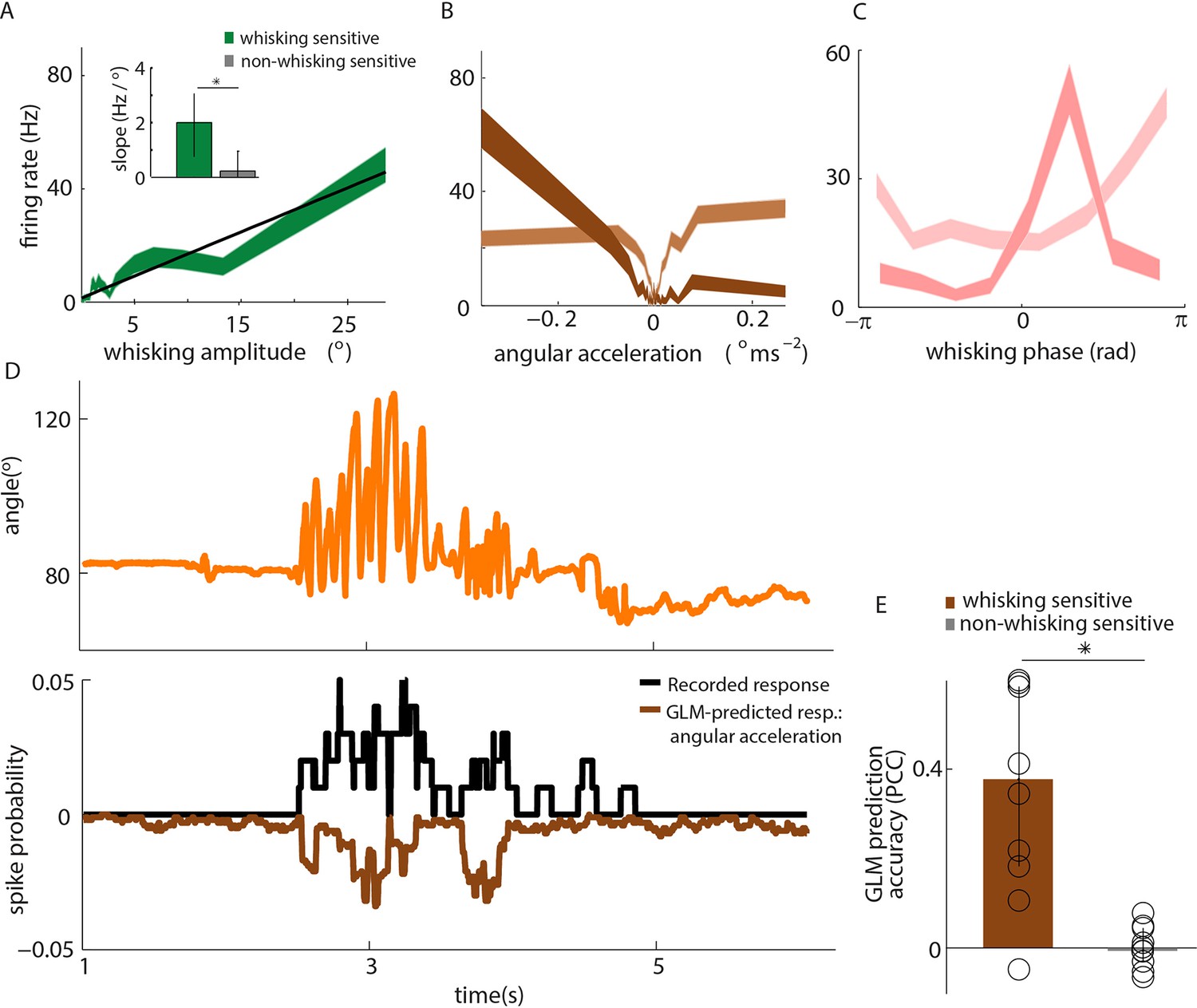
Primary whisker neurons encode whisker angular acceleration during free whisking.
(A) Mean response of an example whisking-sensitive unit to whisking amplitude, computed during non-contact episodes (dark green, shaded area shows SEM) with regression line (black). Inset shows regression line slopes (median and IQR) for whisking sensitive (green) and whisking insensitive (grey) units. * indicates statistically significant rank-sum test (p=0.05). (B) Mean response of two example units as a function of angular acceleration. The dark brown unit is the same as that shown in A. (C) Mean response of two example units as a function of whisking phase. The dark pink unit is the same as that reported in A; the light pink unit is the same as that shown as light brown in B. (D) Excerpt of free whisking (orange) along with activity of an example, whisking-sensitive unit (black) and activity predicted by a GLM driven by angular acceleration (brown). The unit is the same as that shown in A. (E) GLM prediction accuracy (PCC) for all whisking sensitive (brown) and whisking insensitive units (grey). Bars and vertical lines denote median and IQR respectively.
Figure 3—figure supplement 1
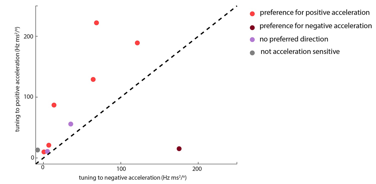
Whisking-sensitive units exhibit heterogeneous selectivity to angular acceleration.
For each whisker-sensitive unit, an acceleration tuning curve was estimated (Figure 3B). Tuning to positive (negative) acceleration was quantified by the slope of a regression line fitted to the positive (negative) half of the acceleration tuning curve. In general, units responded to both positive and negative accelerations, but to different degrees. Statistical tests, based on regression coefficients, detailed in Materials and methods, were used to differentiate the different types of unit.
Figure 4 with 2 supplements

Whisker angle and whisker curvature change are highly correlated during passive whisker deflection, but decoupled during active touch.
(A) Whisker angle (top) and whisker curvature change (bottom) time series, due to passive, trapezoidal stimulation of C2 whisker in an anaesthetized mouse, estimated as mean over 10 repetitions. Note that error bars (showing SEM) are present but very small. (B) Corresponding data for low-pass filtered white noise (hereafter abbreviated to ‘white noise’) stimulation of the same whisker. (C) Cross-correlation between curvature change and angle during white noise stimulation, for C2 whisker. (D) Cross-correlation between angle and curvature change at zero lag, for both passive stimulation under anaesthesia and awake, active sensing (median of absolute cross-correlation for each unit; error bar denotes IQR). (E) Joint distribution of whisker angle and whisker curvature change in awake, behaving mice (1 ms sampling). Different colours denote data corresponding to different recorded units. Inset: Analogous plot for passive, white noise whisker deflection in an anaesthetised mouse. Different colours indicate data from different whiskers. (F) Joint distribution of angle and curvature change for an example recording from an awake behaving mouse, with samples registered during touch and non-touch distinguished by colour (1 ms sampling). (G) Touch data of F classified according to pole position (dot colour).
Figure 4—figure supplement 1
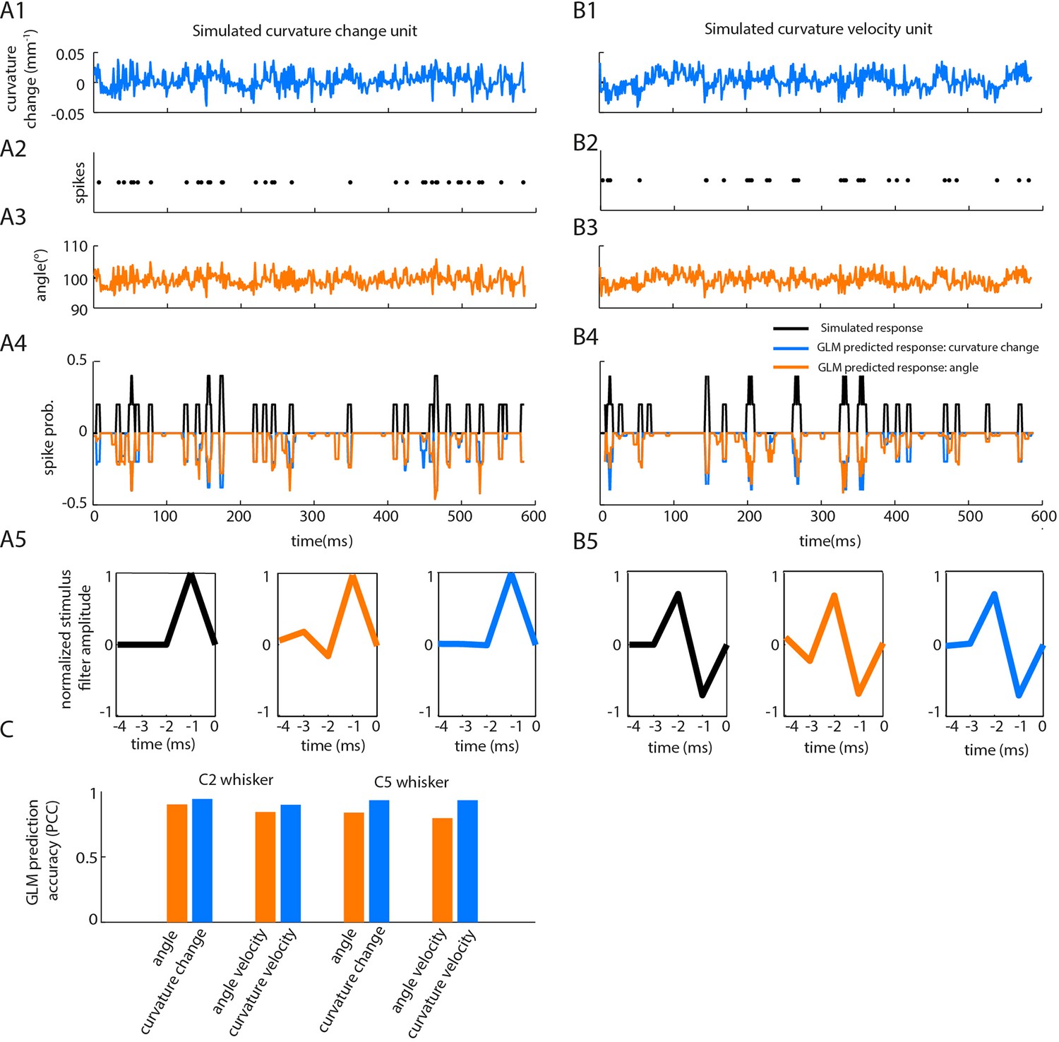
Correlations between angle and curvature change during passive whisker stimulation can make curvature-tuned units appear angle-tuned.
The data of Figure 4 show a strong correlation between whisker angle and whisker curvature during passive stimulation of the whisker. To test whether this correlation might make curvature-tuned units appear angle-tuned, we used a simulation approach. This allowed us to generate responses from idealised neurons whose true tuning was known, by construction, to be only to curvature. We simulated responses of such neurons to the curvature change time series obtained from passive white noise stimulation (A1-2). We then trained a GLM to predict these curvature-evoked spikes using only whisker angle as input (A3-A4). Despite being fed the ‘wrong’ input, this GLM was able to predict the spikes accurately (for C2 whisker, angle PCC was 0.90, curvature change PCC 0.94; results similar for C5; C). This result was robust to different choices of feature tuning (B-C). (A1) Whisker curvature change caused by the white noise stimulus applied to C2 whisker of an anaesthetized mouse (same data as main text Figure 4B, repeated for clarity). (A2) Spike train evoked by a simulated curvature-tuned neuron in response to the stimulus in A1 (a GLM with the position filter shown in left panel of A5). (A3) Whisker angle time series corresponding to panel A1. (A4) Target response (black) compared to predicted response from best-fitting GLMs using either angle (orange) or curvature change (blue) as input. (A5) Left. Stimulus filter used to generate the spike train of panel A2. Middle-Right. Best-fitting stimulus filters (normalised to unit length) for GLMs trained on the spikes of panel A2 and the angle time series of panel A3 or the curvature change time series of panel A1 respectively. (B1-5) Results analogous to A1-5 for a simulated neuron tuned to curvature velocity. (C) Quantification of the GLM predictions shown in panels A4-B4.
Figure 4—figure supplement 2

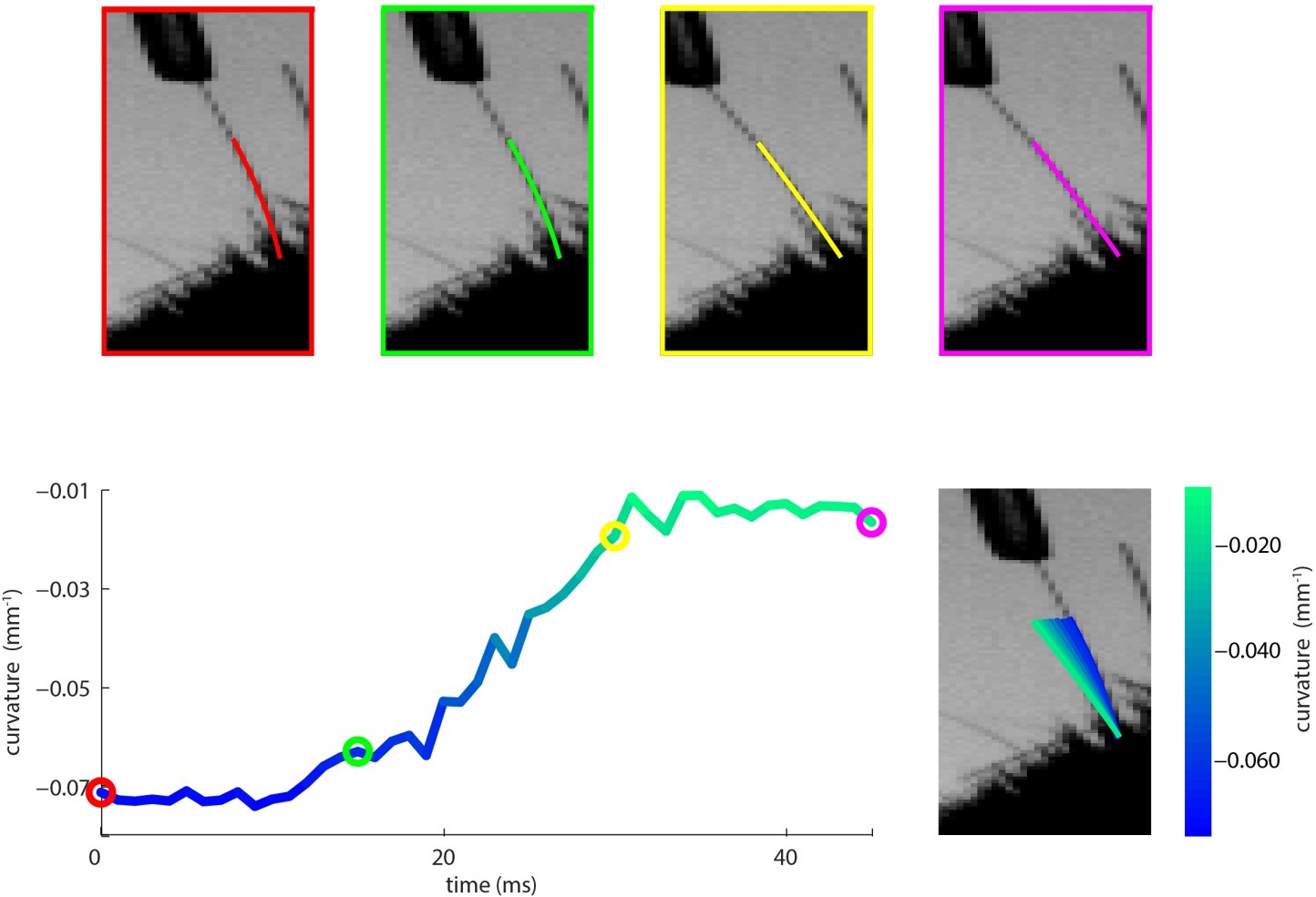
Measurement of whisker bending during passive whisker deflection.
(A). Four video frames taken during trapezoidal, passive whisker stimulation with whisker tracker solutions overlaid (coloured lines). (B) Curvature change (left) and corresponding tracker solutions (right) during a 45 ms episode. Coloured dots mark the times of the example frames in panel A and shading from blue to aqua indicates curvature change. This whisker had negative intrinsic curvature. As the actuator applied force to the whisker, the whisker straightened up and the curvature increased.
Author response image 1
Videos
Video 1
Video of an awake mouse, exploring a pole with its whiskers with simultaneous electrophysiological recording of a primary whisker neuron.
At the start of the video, the pole is out of range of the whiskers. The whisker tracker solution for the principal whisker of the recorded unit is overlaid in red. White dots represent spikes; orange trace shows whisker angle (scale bar = 40°); blue trace shows whisker curvature change (scale bar = 0.05 mm-1). Video was captured at 1000 frames/s and is played back at 50 frames/s. Related to Figure 1.
Download links
A two-part list of links to download the article, or parts of the article, in various formats.
Downloads (link to download the article as PDF)
Open citations (links to open the citations from this article in various online reference manager services)
Cite this article (links to download the citations from this article in formats compatible with various reference manager tools)
Prediction of primary somatosensory neuron activity during active tactile exploration
eLife 5:e10696.
https://doi.org/10.7554/eLife.10696


