Neural precursors of decisions that matter—an ERP study of deliberate and arbitrary choice
- Chapman University, United States
- University of California, Los Angeles, United States
- California Institute of Technology, United States
- Yale University, United States
- Allen Institute for Brain Science, United States
- Tel Aviv University, Israel
Figures
Figure 1

Experimental paradigm.
The experiment included deliberate (red, left panel) and arbitrary (blue, right panel) blocks, each containing nine trials. In each trial, two causes—reflecting NPO names—were presented, and subjects were asked to either choose to which NPO they would like to donate (deliberate), or to simply press either right or left, as both NPOs would receive an equal donation (arbitrary). They were specifically instructed to respond as soon as they reached a decision, in both conditions. Within each block, some of the trials were easy (lighter colors) decisions, where the subject’s preferences for the two NPOs substantially differed (based on a previous rating session), and some were hard decisions (darker colors), where the preferences were more similar; easy and hard trials were randomly intermixed within each block. To make sure subjects were paying attention to the NPO names, even in arbitrary trials, and to better equate the cognitive load between deliberate and arbitrary trials, memory tests (in light gray) were randomly introduced. There, subjects were asked to determine which of four NPO names appeared in the immediately previous trial. For a full list of NPOs and causes see Supplementary file 1.
Figure 2
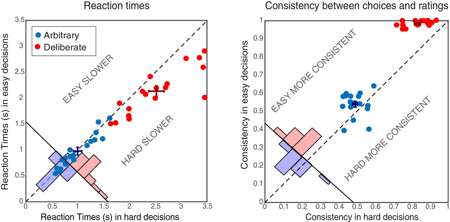
Behavioral results.
Reaction Times (RTs; left) and Consistency Grades (CG; right) in arbitrary (blue) and deliberate (red) decisions. Each dot represents the average RT/CG for easy and hard decisions for an individual subject (hard decisions: x-coordinate; easy decisions: y-coordinate). Group means and SEs are represented by dark red and dark blue crosses. The red and blue histograms at the bottom-left corner of each plot sum the number of red and blue dots with respect to the solid diagonal line. The dashed diagonal line represents equal RT/CG for easy and hard decisions; data points below that diagonal indicate longer RTs or higher CGs for hard decisions. In both measures, arbitrary decisions are more centered around the diagonal than deliberate decisions, showing no or substantially reduced differences between easy and hard decisions.
Figure 3
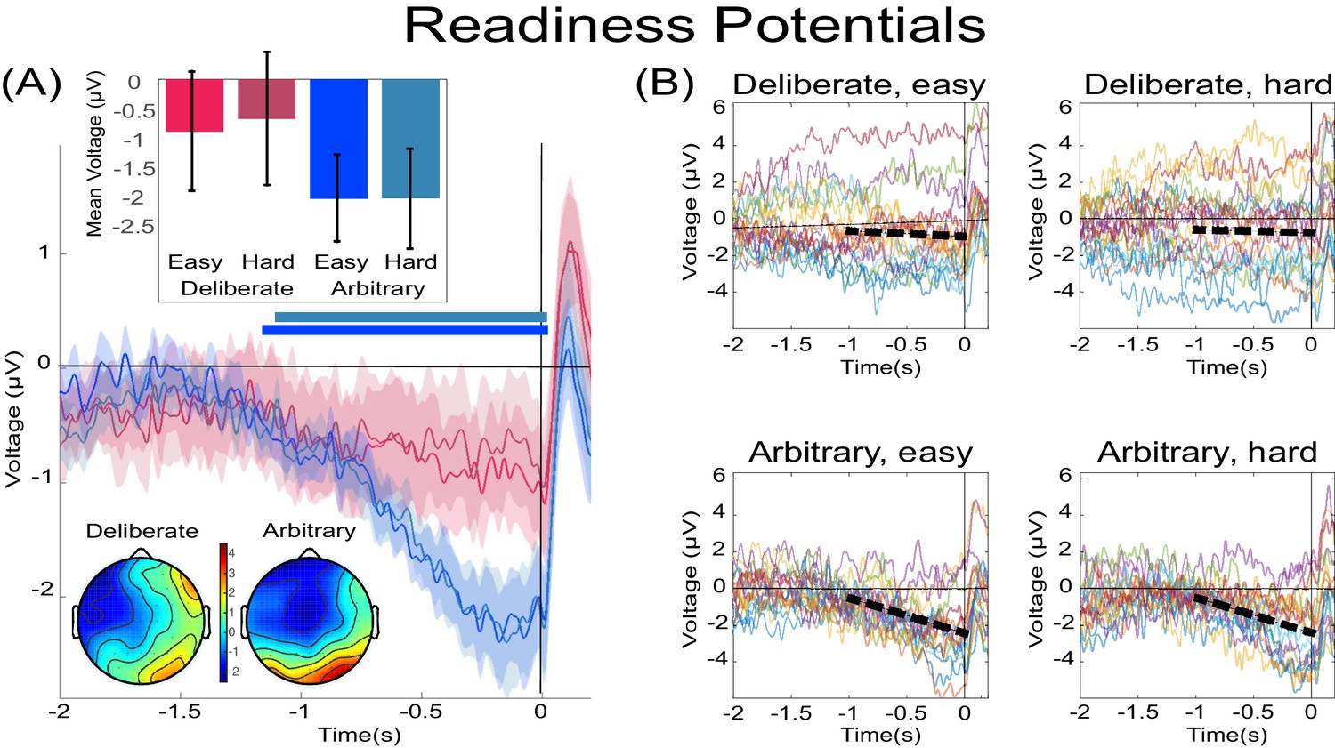
The readiness potentials (RPs) for deliberate and arbitrary decisions.
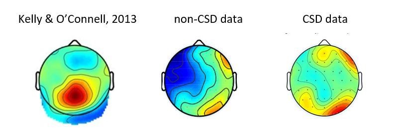
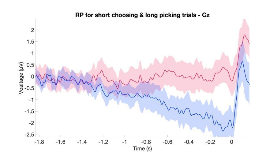
(A) Mean and SE of the readiness potential (RP; across subjects) in deliberate (red shades) and arbitrary (blue shades) easy and hard decisions in electrode Cz, as well as scalp distributions. Zero refers to time of right/left movement, or response, made by the subject. Notably, the RP significantly differs from zero and displays a typical scalp distribution for arbitrary decisions only. Similarly, temporal clusters where activity was significantly different from 0 were found for arbitrary decisions only (horizontal blue lines above the x axis). Scalp distributions depict the average activity between −0.5 and 0 s, across subjects. The inset bar plots show the mean amplitude of the RP, with 95% confidence intervals, over the same time window. Response-locked potentials with an expanded timecourse, and stimulus-locked potentials are given in Figure 6B and A, respectively. The same (response-locked) potentials as here, but with a movement-locked baseline of −1 to −0.5 s (same as in our Bayesian analysis), are given in Figure 6C. (B) Individual subjects’ Cz activity in the four conditions (n = 18). The linear-regression line for voltage against time over the last 1000 ms before response onset is designated by a dashed, black line. The lines have slopes significantly different from 0 for arbitrary decisions only. Note that the waveforms converge to an RP only in arbitrary decisions.
Figure 4
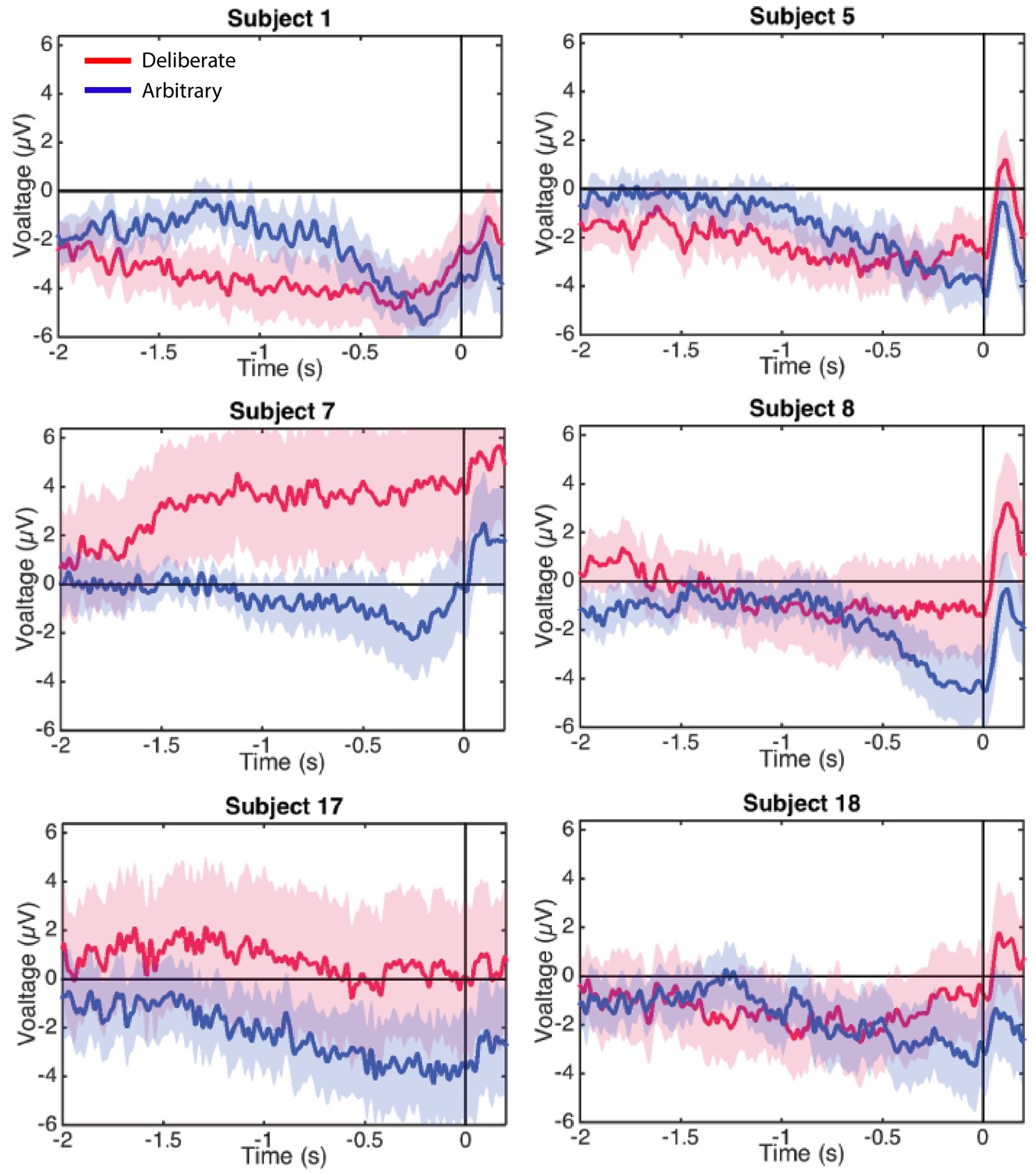
Individual-subjects RPs.
Six examples of for individual subjects’ RPs for deliberate decisions (in red) and arbitrary ones (in blue) pooled across decision difficulty.
Figure 5
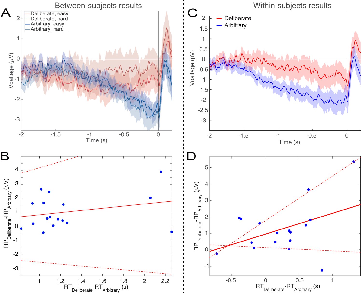
Relations between RTs and RPs between subjects (A and B) and within subjects (C and D).
(A) The subjects with above-median RTs for arbitrary decisions (in blue) and below-median RTs for deliberate decisions (in red), show the same activity pattern that was found in the main analysis (compare Figure 3A). (B) A regression of the difference between the RPs versus the difference between the RTs for deliberate and arbitrary decisions for each subject. The equation of the regression line (solid red) is y = 0.54 [CI −0.8, 1.89] x - 0.95 [CI −2.75, 0.85] (confidence intervals: dashed red lines). The R2 is 0.05. One subject, #7, had an RT difference between deliberate and arbitrary decisions that was more than six interquartile ranges (IQRs) away from the median difference across all subjects. That same subject’s RT difference was also more than 5 IQRs higher than the 75th percentile across all subjects. That subject was therefore designated an outlier and removed only from this regression analysis. (C) For each subject separately, we computed the RP using only the faster (below-median RT) deliberate trials and slower (above-median RT) arbitrary trials. The pattern is again the same as the one found for the main analysis. (D) We computed the same regression between the RP differences and the RT differences as in B, but this time the median split was within subjects. The equation of the regression line is y = 1.27 [CI −0.2, 2.73] x - 0.95 [CI 0.14, 1.76]. The R2 is 0.18.
Figure 6
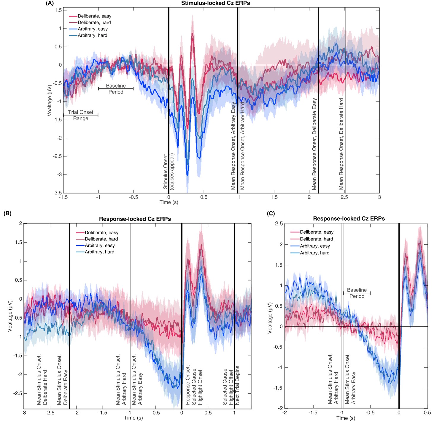
Stimulus- and response-locked Cz-electrode ERPs with different baselines and overlaid events.
(A) Stimulus-locked waveforms including the trial onset range, baseline period, and mean reaction times for all four experimental conditions. (B) Response-locked waveforms with mean stimulus onsets for all four conditions as well as the offset of the highlighting of the selected cause and the start of the next trial. (C) Same potentials and timeline as Figure 3A, but with a response-locked baseline of −1 to −0.5 s—the same baseline used for our Bayesian analysis.
Figure 7
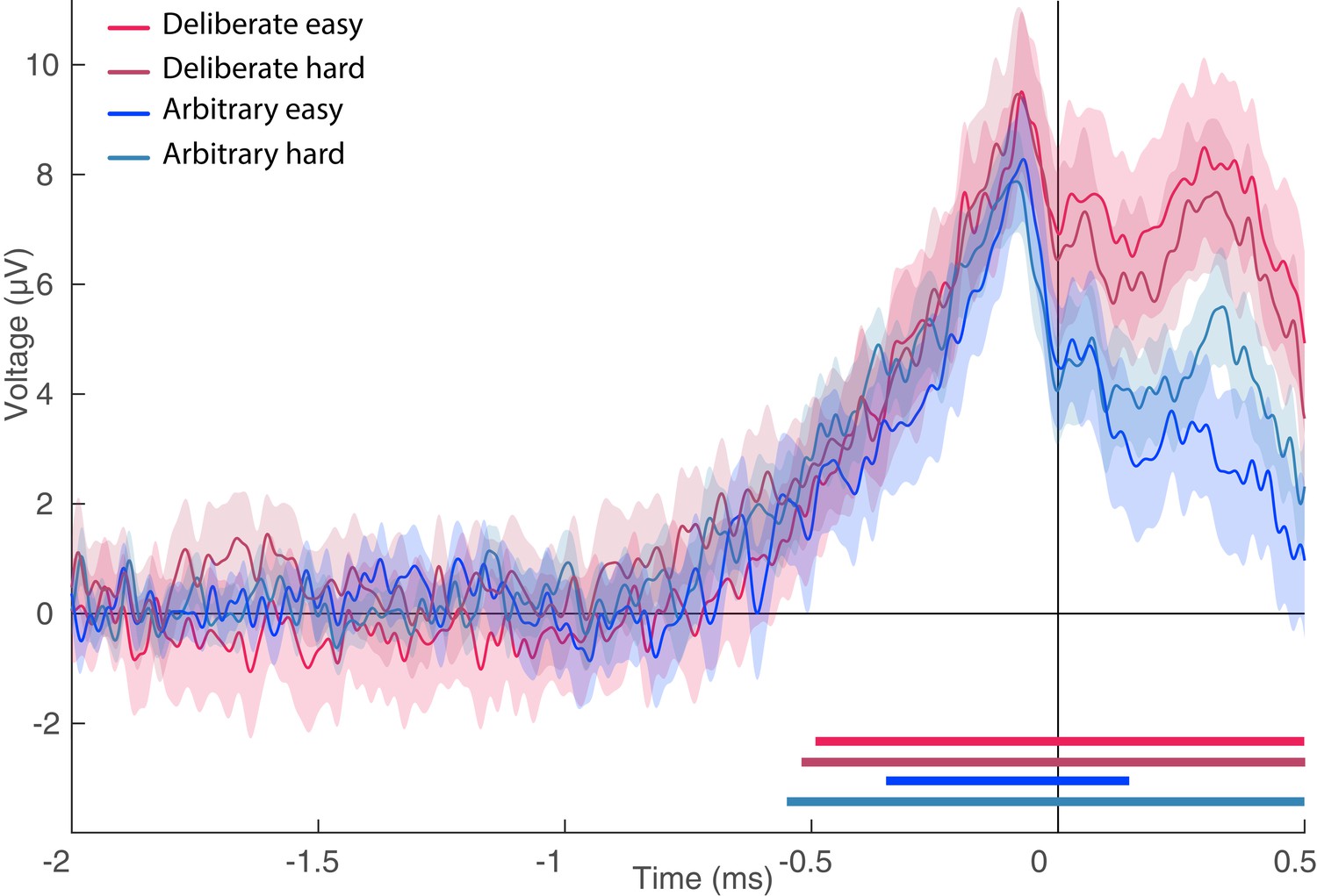
Lateralized readiness potential (LRP).
The lateralized LRP for deliberate and arbitrary, easy and hard decisions. No difference was found between the conditions (ANOVA all Fs < 0.35). Temporal clusters where the activity for each condition was independently found to be significantly different from 0 are designated by horizontal thick lines at the bottom of the figure (with their colors matching the legend).
Figure 8
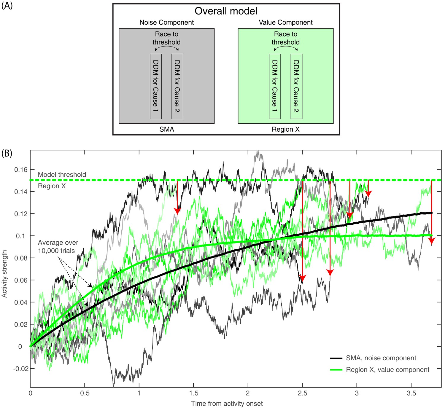
Model description and model runs in the SMA and in Region X.
(A) A block diagram of the model, with its noise (SMA) and value (Region X) components, each instantiated as a race to threshold between a pair of DDMs (or causes—one congruent with the ratings in the first part of the experiment, the other incongruent). (B) A few runs of the model in the deliberate condition, in Region X (green colors), depicting the DDM for the congruent option. As is apparent, the DDM stops when the value-based component reaches threshold. Red arrows point from the Region X DDM trace at threshold to the corresponding time in the trace of the SMA (black and gray colors). The SMA traces integrate without a threshold (as the decision outcome is solely determined by the value component in Region X). The thick green and black lines depict average Region X and SMA activity, respectively, over 10,000 model runs locked to stimulus onset. Hence, we do not expect to find an RP in either brain region. (For decision-locked activity see Figure 9B).
Figure 9
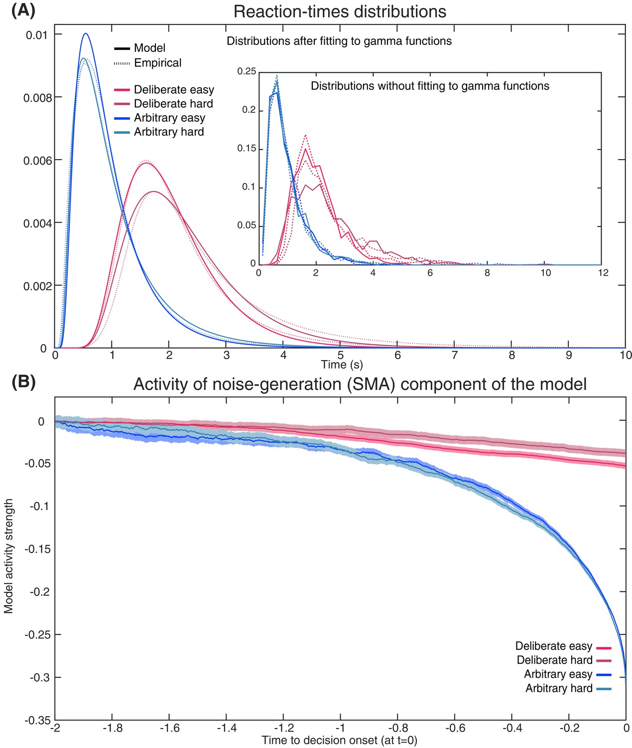
Empirical and model RTs and model prediction for Cz activity.
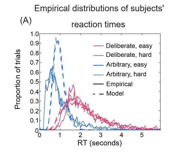
(A) The model (solid) and empirical (dashed) distributions of subjects’ RTs. We present both the data as fitted with gamma functions to the cumulative distributions (see Materials and methods) across the four decision types in the main figure, and the original, non-fitted data in the inset. (B) The model’s prediction for the ERP activity in its Noise Component (Figure 8A) in the SMA (electrode Cz), locked to decision completion (at t = 0 s), across all four decision types.
Author response image 1
Author response image 2
Author response image 3
Tables
Table 1
Values of the model’s parameters across decision types and decision difficulties.
Values of the drift-rate parameter, I, for the congruent and incongruent options; for the leak rate, k; and for the noise scaling factor, c. We fixed the threshold at the value of 0.3. The values in the table are for the component of the model where the decisions were made. Hence, they are for Region X in deliberate decisions and for the SMA in arbitrary ones. Note that, for deliberate decisions, drift-rate values in the SMA were 1.45 times smaller than the values in this table for each entry.
| Decision type | Decision difficulty | Icongruent | Iincongruent | K | C |
|---|---|---|---|---|---|
| Deliberate decisions (Region X values) | Easy | 0.23 | 0.06 | 0.52 | 0.08 |
| Hard | 0.18 | 0.09 | 0.53 | 0.11 | |
| Arbitrary decisions (SMA values) | Easy | 0.24 | 0.21 | 0.53 | 0.22 |
| Hard | 0.22 | 0.20 | 0.54 | 0.23 |
Additional files
-
Supplementary file 1
NPO names and causes acronyms.
- https://doi.org/10.7554/eLife.39787.012
-
Transparent reporting form
- https://doi.org/10.7554/eLife.39787.013
Download links
A two-part list of links to download the article, or parts of the article, in various formats.
Downloads (link to download the article as PDF)
Open citations (links to open the citations from this article in various online reference manager services)
Cite this article (links to download the citations from this article in formats compatible with various reference manager tools)
Neural precursors of decisions that matter—an ERP study of deliberate and arbitrary choice
eLife 8:e39787.
https://doi.org/10.7554/eLife.39787


