Rodent ultrasonic vocal interaction resolved with millimeter precision using hybrid beamforming
- Computational Neuroscience Lab, Donders Institute for Brain, Cognition and Behaviour, Radboud University Nijmegen, Netherlands
- Visual Neuroscience Lab, Donders Institute for Brain, Cognition and Behaviour, Radboud University Nijmegen, Netherlands
- Department of Human Genetics, Radboudumc, Donders Institute for Brain, Cognition and Behaviour, Radboud University Nijmegen, Netherlands
Figures
Figure 1 with 1 supplement
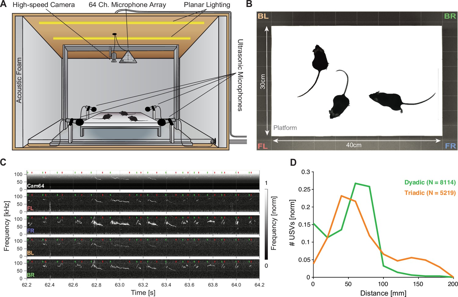
Mice emit ultrasonic vocalizations (USVs) in close proximity during courtship behavior.
(A) Two or three mice of different sexes were allowed to interact freely on an elevated platform. Vocalizations were recorded with four high-quality ultrasonic microphones in a rectangular arrangement around the platform and a 64-channel microphone array ('Cam64') mounted above the platform. The spatial location of the pair was recorded visually with a high-speed camera. The platform was located in an ultrasonically sound-proof and anechoic box and illuminated uniformly using an array of LEDs. (B) Sample image from the camera that shows the high contrast between the mice and the interaction platform. The two-letter abbreviations indicate the locations of the four high-quality microphones (F = front, B = back, L = left, R = right). (C) Sample spectrograms from the four ultrasonic microphones and the average of all Cam64 microphones for a bout of vocalizations (start/end times marked by green/red dots). The Cam64 microphones are of lower quality than the USM4 microphones, evidenced by the rising noise floor for higher frequencies, affecting very-high-frequency USVs. (D) Most USVs in the present paradigm were emitted in close proximity to the interaction partners, with the vast majority within 10 cm snout–snout distance (i.e., ~93 and 72% for dyadic and triadic, respectively).
Figure 1—figure supplement 1
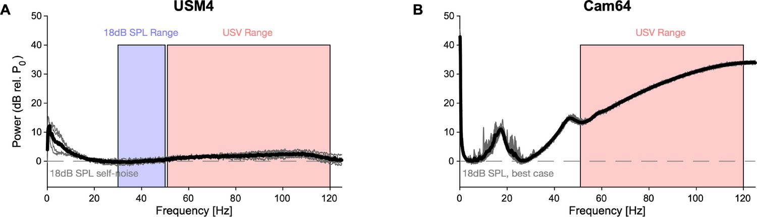
Comparison of noise spectra of the two microphone arrays.
Spectra are computed from the output voltage of the microphones during the same silent stretch of a recording (duration: 1 s, M82,R41, T = [150,151] s), verified to not contain any discernible vocalizations, footsteps, or other discrete sounds. (A) The high-quality ultrasonic microphones (gray: 4× individual, black: average) had a rather flat baseline noise level across frequency, with the only exception of an ~10 dB deviation for low frequencies, far below the relevant frequency range contained in USVs (red overlay). For reference, the spectrum was shifted to the average of the power in the 30–50 kHz range (blue overlay), which is listed in the manual as being the ‘input-referred self-noise level,’ corresponding to 18 dB SPL (http://www.avisoft.com/ultrasound-microphones/cm16-cmpa/). (B) The Cam64 micro-electromechanical systems (MEMS) microphones (gray: 64× individual, black: average, Akustica AKU242) have a highly frequency-dependent baseline noise across frequency. The peaks at frequencies <50 kHz are less relevant for USV detection, while the substantial rise of the noise level for higher frequencies poses an issue for detecting very high frequencies as their contribution to the recorded signal gets progressively buried in the baseline noise (see Figure 1C for the effect on the detectability of high-frequency USVs). Since no information was available on the input-referred self-noise level in the technical documentation, we shifted the curve to its minimum. In reality it should be shifted higher to be quantitatively compared with the Avisoft microphone as the latter’s large membrane is expected to outperform the AKU242 at all frequencies. For clarity, the above spectra are not equivalent to the sensitivity of the microphone at different frequencies; however, the baseline noise limits the sensitivity at these frequencies. While in principle a frequency-dependent increase in sensitivity could overcome the baseline noise, this does not seem to be the case (see Figure 1C, top).
Figure 2
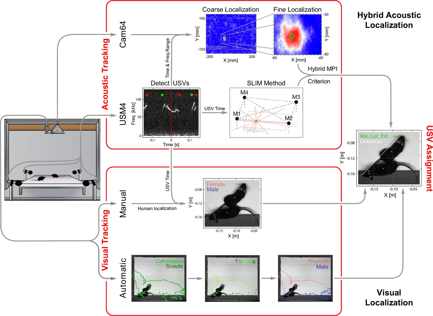
Overview of the combined acoustic and visual tracking pipeline.
(Top) Acoustic tracking of animal vocalizations was enabled by a hybrid acoustic system, which recorded the sounds in the booth using a 64-channel ultrasonic microphone array ('Cam64') and four high-quality ultrasonic microphones ('USM4'). Vocalizations were automatically detected using USM4 data (start/end times marked by green/red dots) and then localized on the platform using both the SLIM algorithm on USM4 data and delay-and-sum beamforming on the corresponding Cam64 data. The Cam64 localization proceeded in two steps: first coarse (10 mm resolution), then fine centered around the coarse peak at 1 mm resolution (30 × 30 mm local window). The local, weighted average (green circle) was then used as the ultrasonic vocalization (USV) origin localized by Cam64. For each USV, the Cam64 localization was chosen if its SNR >5, otherwise the USM4/SLIM estimate was used (for details, see ‘Localization of ultrasonic vocalizations’). (Bottom) Animals were tracked visually on the basis of concurrently acquired videos. Two tracking strategies were employed: (i) manual tracking in the video frames corresponding to the midpoint of USVs in all recordings and (ii) automatic tracking for all frames in dyadic recordings. (i) Manual visual tracking: the observer was presented with a combined display of the vocalization spectrogram and the concurrent video image at the temporal midpoint of each USV and annotated the snout and head center (i.e., midpoint between the ears). (ii) Automatic visual tracking: started with finding the optimal locations of each marker based on marker estimate clouds produced by DeepLabCut (Mathis et al., 2018) (DLC) for all frames. Next, these marker positions were assembled into spatiotemporal threads with the same, unknown identity based on a combination of spatial and temporal analysis. Finally, the thread ends still loose were connected based on quadratic spatial trajectory estimates for each marker, yielding the complete track for both mice (see ‘Automatic visual animal tracking’ and Figure 3—figure supplement 1).
Figure 3 with 3 supplements
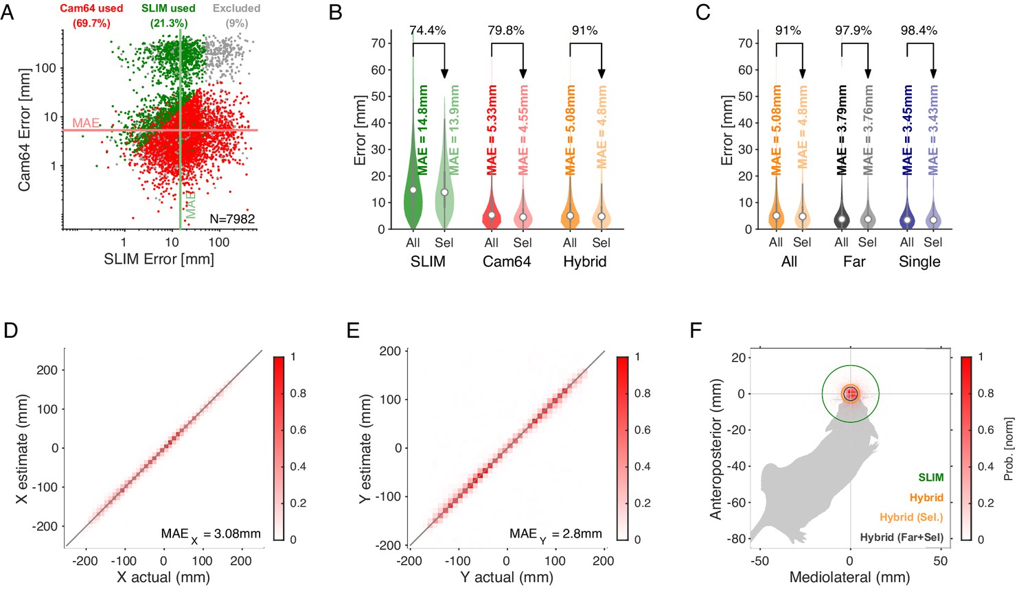
Spatial accuracy of localizing ultrasonic vocalizations (USVs) during mouse social interaction improves approximately threefold over the state of the art (Oliveira-Stahl et al., 2023).
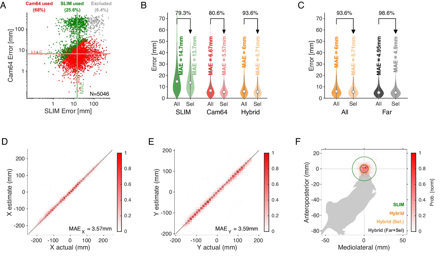
(A) The vast majority of USVs is localized with very small errors for both methods, concentrated close to the axes and thus hardly visible, evidenced by the median absolute errors (MAE) for Cam64 (light red line) and SLIM (light green line). The fewer larger errors form an L-shape, emphasizing the synergy of a hybrid approach that compensates for the weaknesses of each method. Location estimates were excluded (gray) if they were >50 mm from either mouse, or the hybrid Mouse Probability Index (MPI) <0.95. (B) The hybrid localization system Hybrid Vocalization Localizer (HyVL) (orange) combines the virtues of SLIM and Cam64 enabling the localization of 91.1% of all USVs (light orange), achieving an MAE = 4.8 mm. Cam64 localization (red) alone only includes 74.4% of all USVs, but at an MAE = 4.55 mm (light red). SLIM-based localization (green) only includes 79.8% of all USVs, at an MAE = 14.8 mm (light green, see ‘USV assignment’ for details on the relation between accuracy and selection criteria). (C) USVs emitted when all animals were >100 mm apart and a single mouse condition was used to assess the ideal accuracy of HyVL. For the far condition, virtually all USVs (332/339, 97.9%) were assigned at an MAE = 3.79 mm, similarly to the single animal condition (MAE = 3.45 mm, 251/255, 98.4%). (D, E) Comparison of actual with estimated snout locations along the X (horizontal; D) and Y (vertical; E) dimensions indicating strong agreement. Colors indicate peak-normalized occurrence rates. (F) Centered overlay of USV localizations relative to emitter snout. Precision is depicted as a circle with a radius equivalent to the median absolute error (green: SLIM; orange: HyVL, all USVs; light orange: HyVL, selected USVs, dark gray: HyVL, when mice >100 mm apart).
Figure 3—figure supplement 1

Schematic depiction of the progression of marker localization and identity attribution.
(A) First, unattributed estimate clouds (i.e., not assigned to an animal) for each of the six markers are collected using DeepLabCut (DLC). Within each marker class, all estimates are treated as identical at this point (colors indicate marker class). (B) Optimal marker locations are then generated by within-frame, k-means clustering of the estimate clouds, or if that results in an incorrect number of clusters, by probability-weighted averaging of estimate clouds heuristically separated by animal. (C, D) Next, all markers undergo a temporal and spatial analysis in tandem, both with the goal of constructing pieces of unattributed tracks. (C) In the temporal analysis, small spatiotemporal threads of marker locations are assembled and assessed in terms of speed and acceleration to extend them as much as possible across neighboring frames. (D) In the spatial analysis, all marker positions are analyzed spatially on a frame-by-frame basis, grouping markers with the same identity based on a logical combination of anatomically permitted inter-marker distances. (E) Finally, complete, attributed tracks are constructed by combining both analyses (see ‘Automatic visual animal tracking’). For actual data, the analysis is less ideal than in the figure: not all markers necessarily have an estimate cloud representing them all the time, nor are the estimates always accurate. The finished tracks were visually checked and corrected if necessary (~10 corrections per trial on average, a major reduction).
Figure 3—figure supplement 2
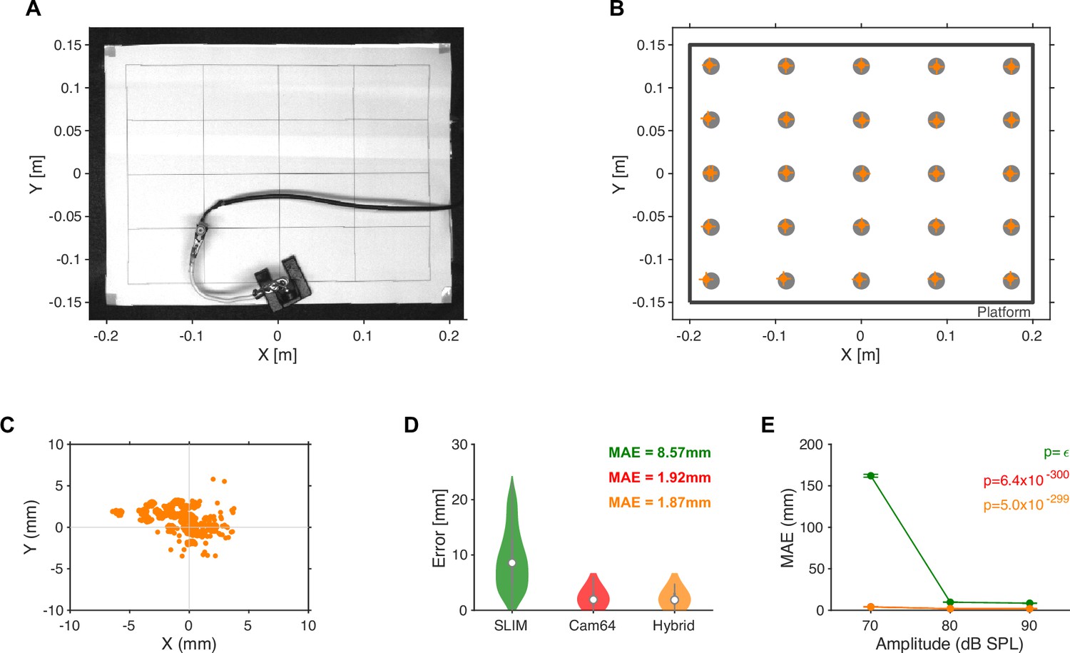
Ground truth localization of band-limited noise emitted from a small speaker.
(A) Noise target sounds were presented from 25 locations arranged in a 5 × 5 grid spanning nearly the size of the interaction platform. A speaker was manually placed at each location and 100 repetitions of a band-limited noise sound (50–75 kHz) for three intensities ([70,80,90] dB SPL, measured at the speaker) were presented from a miniature high-quality in-ear driver (Sennheiser IE800, calibrated up to 80 kHz). Due to the physical size of the speaker, its membrane was located ~4 cm above the platform, which was taken into account in the source localization. The video shown was slightly corrected for lens distortions to exhibit orthogonal/parallel lines on the placement grid (see ‘Materials and methods’). (B) The accuracy of the Hybrid Vocalization Localizer (HyVL) estimates (orange) at each location (gray dots) was quite similar, after minor, linear rescaling (~2% in both directions) and residual shifting (4.5 mm in x, error bars show x and y [17,83] percentiles around the median). The remaining shifts in, for example, the lower left corner could partly be due to slight misplacements of the speaker. (C) Density of estimates centered on known speaker locations. The errors group around the individual locations, while the variance inside the groups is below a single millimeter. This further suggests that the main source of shifts was imperfect placements/orientation of the speaker. (D) The HyVL-based source locations estimates were largely dominated by the Cam64 estimates (96.2%) leading to an accuracy of 1.87 mm, compared to 8.57 mm for SLIM and 1.92 for Cam64 alone. (E) As expected, the accuracy of localization depended on the sound intensity (p<<0.001 for all methods, Kruskal–Wallis ANOVA). As mice are known to vocalize with ~60–100 dB SPL (Portfors and Perkel, 2014), this is in line with our ability to localize most vocalizations during social interactions. We estimate that at the distance to the Cam64 (42.5 cm above the speaker), the sound intensity would have been reduced by ~26 dB.
Figure 3—figure supplement 3
Localization results on the basis of automatic tracking from dyadic and triadic recordings.
Figure 4 with 1 supplement
Analysis of sex-dependent vocalizations can depend on localization accuracy.
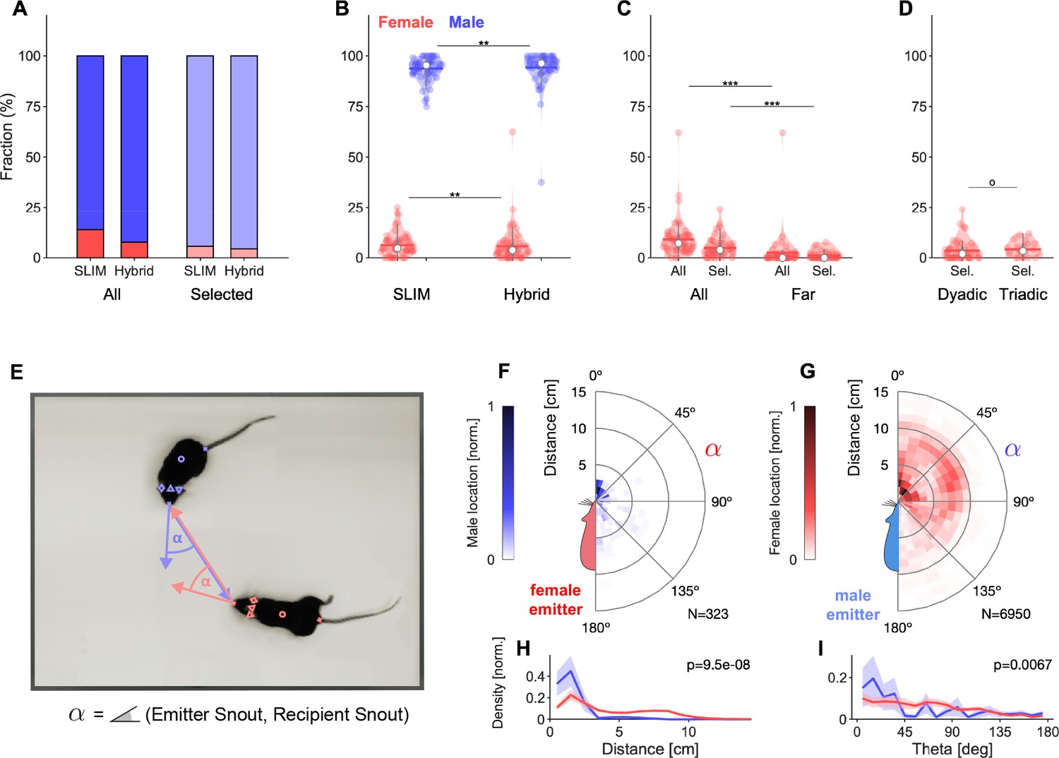
(A) Female vocalizations constitute a small fraction of the total set of vocalizations. The female fraction further reduces with increased precision and when selecting vocalizations based on the Mouse Probability Index (MPI). Vocalization fractions are separated by sex, not by individual mouse. Fractions include all dyadic and triadic recordings with ultrasonic vocalizations (USVs) (N = 83), same for all other panels. (B) Using the hybrid method instead of SLIM significantly reduces the fraction of female vocalizations, suggesting that less accurate algorithms overestimate the female fraction (only results for MPI-selected USVs shown). (C) The fraction of female vocalizations further reduces if only USVs are considered that are emitted while all animal snouts were >50 mm apart from each other. This indicates a preference of female mice to vocalize in close snout–snout contact; however, this entails that female vocalizations are more prone to confusion with male vocalizations due to their relative spatial occurrence. (D) There was no difference in the female fraction of USVs between dyadic and triadic pairings (two male and two female conditions combined here; NDyadic = 55, NTriadic = 28). (E) High-accuracy localization of USVs allows one to analyze the relative spatial vocalization preferences of the mice, that is, their occurrence density in relation to the relative position of other mice to the emitter. We quantified this by collecting the position of the nonvocalizing mice at the times of vocalization, in relation to the vocalizing mouse. Symbol α corresponds to the angle between the emitter’s snout and the snout of other mice. (F) Female mice appear to emit vocalizations in very close snout–snout contact, with a small fraction of vocalizations also occurring when the male mouse around the hind-paws/ano-genital region. (G) Male mice emit vocalizations both in snout–snout contact, but also at greater distances, which dominantly correspond to a close approach of the male’s snout to the female ano-genital region. This was verified separately with a corresponding analysis, where the recipient’s tail-onset was used instead (not shown). (H) Radial distance density of receiver animals, marginalized over directions, shows a significant difference, with females vocalizing mostly when males (blue) are in close proximity of the snout, while males vocalize when the female mouse’s snout is very close (corresponding to snout-snout contact), but also when the female’s snout is about 1 body length away (snout–ano-genital interaction). Plots show means and SEM confidence bounds. (I) Direction density of receiver animals, marginalized over distances, shows that female mice vocalize primarily when the male mouse’s snout is very close and in front of them. Note that the overall angle of approach of the male mouse is not from directly ahead (see Figure 4—figure supplement 1).
Figure 4—figure supplement 1

Relative spatial vocalization preferences relative to receiver’s ano-genital region for dyadic recordings.
(A) The male abdomen is found in a range of different relative locations to the female's snout. (B) A large fraction of the male vocalizations are emitted when the female mouse's abdomen is very close to the male’s snout. (C) Radial distance density of receiver animals, marginalized over directions, shows a significant difference, with males vocalizing mostly (red) when the female abdominal region is in close proximity of their snout (corresponding to snout-ano-genital contact), while females vocalize when the male’s abdomen is relatively far from their snout. Plots show means and SEM confidence bounds. (D) Direction density of receiver animals, marginalized over distances, shows that male mice vocalize (red) primarily when the female’s abdomen is directly in front of them.
Figure 5 with 1 supplement
In triadic interaction, one male vocalizes dominantly and males vocalize even closer to females.
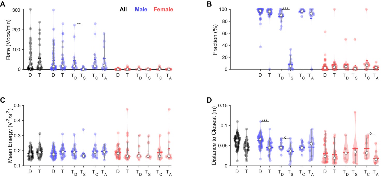
(A) Overall, vocalization rates were comparable between dyadic (D) and triadic (T) conditions. Male mice (blue) vocalized at higher rates than female mice (red). However, this was restricted to the dominant male mouse (TD: dominant = emitted more ultrasonic vocalizations [USVs] within same-sex) in triadic, competitive (2 m/1 f) conditions (see text for all p-values). Male vocalization rates were similar in competitive (TC: with same-sex competitors) and alternative (TA: no same-sex competitor, i.e., for male vocs: 2 f/1 m) pairings. Female vocalization rates remained low and similar across all conditions. TS: submissive mouse = emitted fewer USVs within same sex during competitive trial; white dot: median; horizontal bar: mean (N = 83 recordings in all panels, in the groupings D/T vocalizations are grouped by sex, whereas in TD,S,C,A USVs are per individual, same in panels B–D). (B) While the fraction of USVs emitted by males was overall comparable between D and T pairings, the dominant male (TD) emitted a substantially larger fraction than their submissive counterpart (TS), roughly a factor of 9. In competitive pairings, male mice tended to emit an overall larger fraction of all USVs than in alternative pairings (TC vs. TA), but this is unsurprising as both males vocalize. In female mice, the overall fraction of USVs in D and T pairings was also similar (see details in ‘Results’ for potential caveats of the dominant/subordinate classification). (C) In triadic pairings, dominant male mice tended to vocalize more intensely than in dyadic pairings; however, this difference was not significant at the current sample size. No significant differences were found for female mice. (D) Male mice emitted USVs in closer proximity to the closest female mouse in triadic compared to dyadic interactions. Female mice generally emitted USVs at closer distances (see also Figure 4F/H), in particular for alternative vs. competitive pairings.
Figure 5—figure supplement 1

Vocalization rates in dyadic recordings based on a balanced set of four recordings per male mouse and condition (n = 14 male mice, 112 recordings).
Vocalization rate did not depend significantly on individual for males (A, p=0.46, one-way ANOVA with factor individual, n = 4 recordings per animal) or females (B, p=0.16, one-way ANOVA with factor individual, n = 14 recordings per animal).
Figure 6
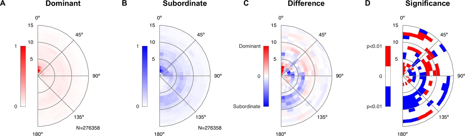
Dominant male animals spend more time close to the female’s abdomen.
(A) The abdomen of the female was typically close to the dominant male’s snout (center of plot), with a ring of approximately one mouse length also visible deriving from snout–snout interactions. The histogram was created based on all-frame tracking of the 14 triadic interactions with two male mice using skeleton tracking in SLEAP over a total of N = 276,358 frames. Dominant and subordinate males were defined based on their vocalization rate per recording. Each histogram was peak normalized. (B) For the subordinate male, the histogram was less peaked around the proximal snout–abdomen interactions, but showed a more visible arc between 90 and 180°, pointing to snout–snout interactions. (C) The difference between the two histograms (each density-normalized to a sum of 1) shows the focused snout–abdominal interactions for the dominant male, and the arc pointing to snout–snout interactions for the subordinate male, in addition to smaller absolute differences in other relative locations. (D) Spatial regions of significant difference between the dominant and subordinate male were found both in the regions highlighted in (C), as well as more distant regions. Significance was assessed by bootstrapping confidence bounds on the histograms of the dominant and subordinate males (based on relative locations, rebuilding the histogram, 100×). The distance to the most extreme values were taken as the limits for significant deviation at p<0.01, and the difference in (C) was then compared in both the positive/negative direction against these bounds.
Videos
Video 1
Example of Hybrid Vocalization Localizer (HyVL) tracking and sound localization.
Marker color represents animal sex (light blue: male; light red: female). Marker shape represents body part (circle: body center; cross: snout or tail; downward triangle: left ear; upward triangle: head center; diamond: right ear). Cam64 ultrasonic vocalization (USV) localizations (yellow) are overlaid on the beamforming densities (red) that are often very narrow and therefore hard to see underneath the localization marker (yellow dot). SLIM USV localizations are shown as well (orange '+'), typically further away from the snout in comparison to Cam64-based localization markers.
Tables
Key resources table
| Reagent type (species) or resource | Designation | Source or reference | Identifiers | Additional information |
|---|---|---|---|---|
| Transfected construct (Mus musculus) | Foxp2flox/flox;Pcp2Cre | Bred locally at animal facility |
Additional files
Download links
A two-part list of links to download the article, or parts of the article, in various formats.
Downloads (link to download the article as PDF)
Open citations (links to open the citations from this article in various online reference manager services)
Cite this article (links to download the citations from this article in formats compatible with various reference manager tools)
Rodent ultrasonic vocal interaction resolved with millimeter precision using hybrid beamforming
eLife 12:e86126.
https://doi.org/10.7554/eLife.86126


