Spatial cue reliability drives frequency tuning in the barn Owl's midbrain
- Albert Einstein College of Medicine, United States
- Seattle University, United States
Figures
Figure 1

Cue variability in the sound localization system.
(A) Tuning to interaural time difference (ITD) emerges from the convergence of inputs selective for the same ITD but different frequencies (F1–F3) (Takahashi and Konishi, 1986; Mazer, 1998; Pena and Konishi, 2000; best ITD indicated by the dashed line). While ITD-selective neurons respond to a broad range of frequencies (here the black bold curve represents the neuron's combined response for frequencies F1, F2 and F3), their inputs are narrowly tuned to frequency (each input only responding to F1, F2 or F3). Because the inputs are narrowly tuned to frequency, the responses at each input vary with the phase difference between the left and right ears (IPD) of their preferred frequency, as shown by the sinusoidal curves. (B) A sound emitted by a single source (B, left) in front of the owl is filtered by the head and decomposed in narrow frequency channels by the cochlea. The localization cue corresponds to an IPD in each frequency channel (F1–F3). In a different context (B, right), the target frontal sound (yellow) is emitted concurrently with another sound source from a different location (blue). The blue source interferes with the yellow target and shifts the resultant IPDs in each frequency channel (shown in green). Black dotted lines indicate IPD responses for the target frontal source alone, for comparison. While IPD shifts greatly for some frequencies (F1 and F3), in others (F2) IPD is more robust to the presence of another source. Thus in this example, F2 carries the most reliable IPD cue. To provide a clearer visualization that IPD is encoded at different frequencies, F1–F3 inputs remain plotted as a function of ITD in (B).
Figure 2
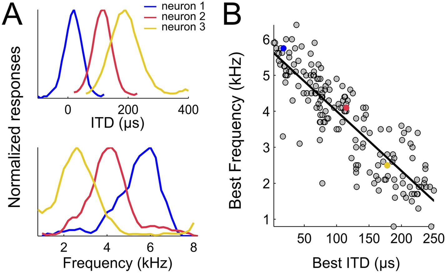
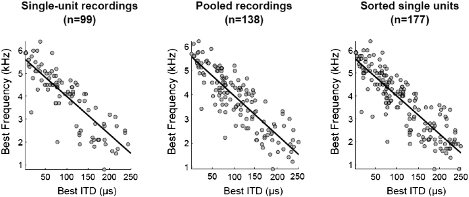
Spatial-dependence of frequency tuning in the population of ICx neurons.
(A; top) ITD tuning measured with broadband noise of three example neurons tuned to 0 µs (blue), 100 µs (red) and 200 µs (yellow). (A; bottom) The frequency tuning, measured with tones at the best ITD shows that best frequencies (BF) decrease as best ITD increases for each neuron (BFs of the shown examples are 6 kHz (blue), 4 kHz (red) and 2 kHz (yellow)). (B) BF decreases with best ITD across the sample of ICx neurons. Linear regression is indicated by a solid line.
Figure 3
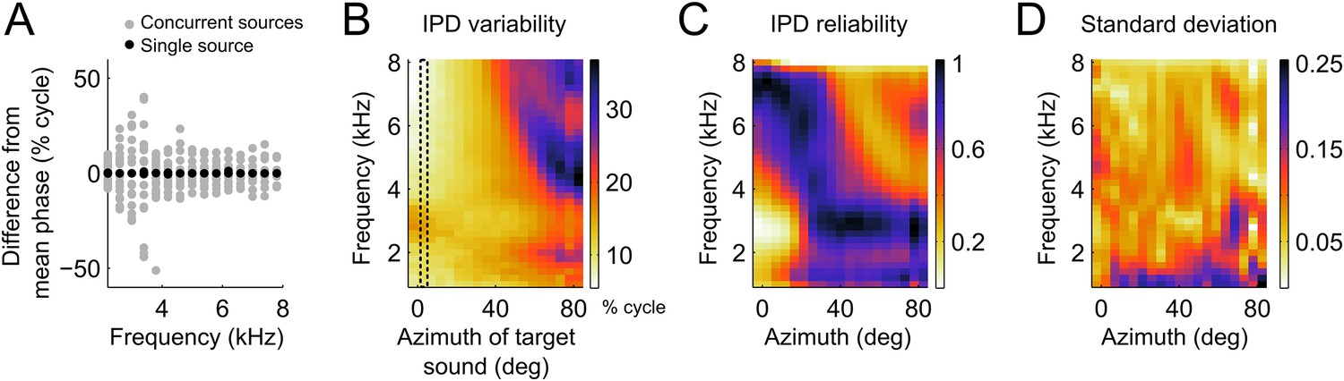
IPD variability computed from the head filters.
(A) Example IPD variation around the mean (normalized to zero for clarity) as a function of frequency when a sound is presented near the front (black dots) and when a second sound source is added from various locations between −90 and 90° (gray dots). Note the larger scatter of gray dots in the lower frequencies (B) IPD standard deviation over concurrent sound sources across frequency at the location of the target sound. The dotted lines show the location of the target sound in (A). In (A) and (B) units are percent of cycle. (C) IPD reliability across location and frequency, normalized by the maximum at each location. (D) Standard deviation of the IPD reliability across HRTFs from 10 different owls. Note that the same colors map the values 0 (least reliable IPD) to 1 (most reliable IPD) in C and 0–0.25 in D.
Figure 4
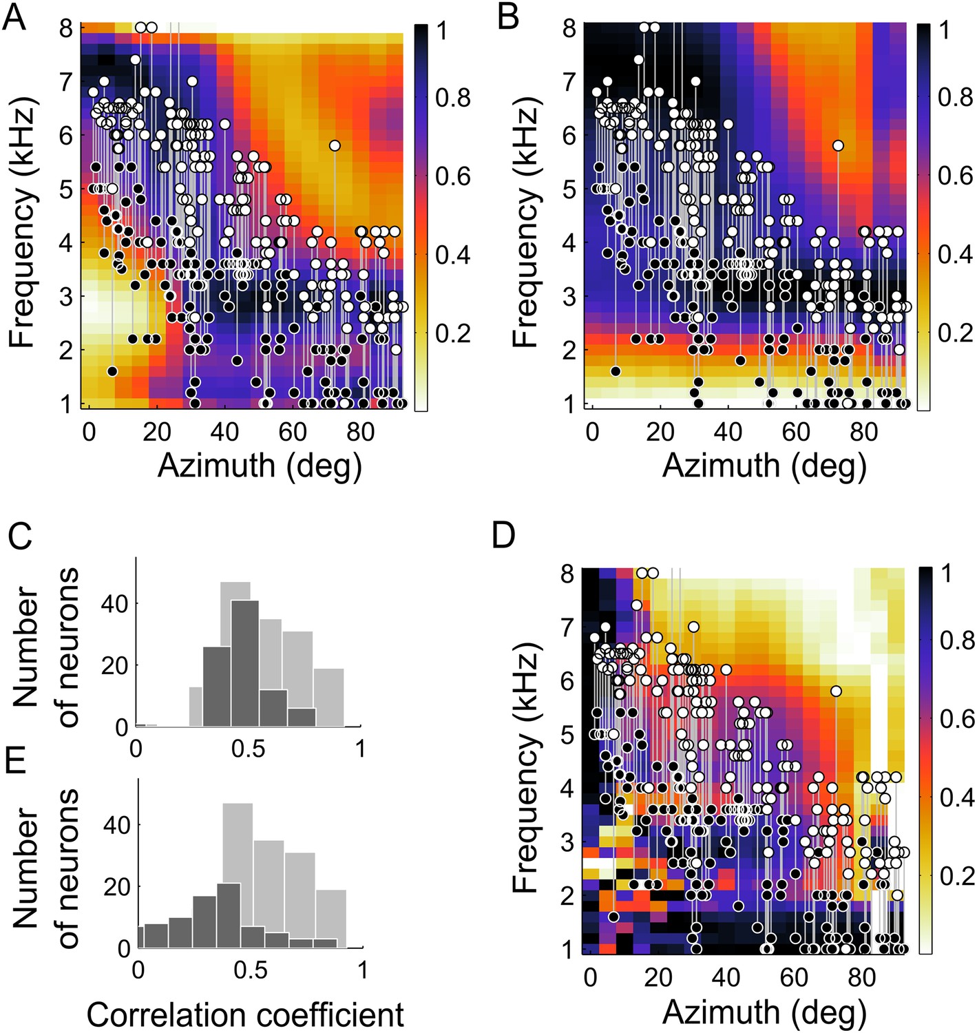
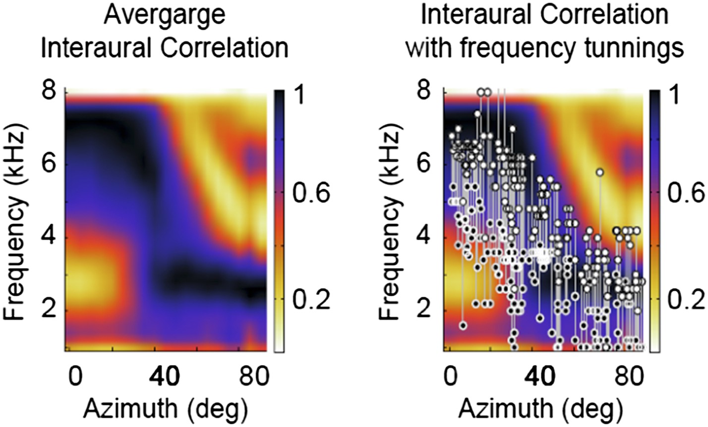
Frequency tuning in ICx matches IPD reliability.
(A) Upper (white circles) and lower (black circles) edges of frequency tuning of ICx neurons superimposed on the plot of IPD-reliability. (B) Upper and lower boundaries of frequency tuning superimposed on the average gain normalized at each location (from 0 to 1). (C) The correlation coefficients between frequency tuning curves and frequency tuning predicted by the IPD-reliability (gray) are higher than the correlation coefficients between frequency tuning curves and gain alone (black). (D) Upper and lower edges of frequency tuning superimposed on the average gain normalized successively at each frequency and at each location (from 0 to 1). (E) The correlation coefficients between frequency tuning curves and frequency tuning predicted by the IPD-reliability (gray) are higher than the correlation coefficients between frequency tuning curves and the normalized gain (black).
Figure 5
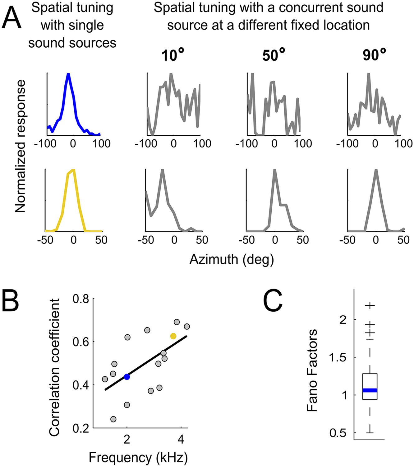
Testing the weighting by reliability hypothesis.
(A) The colored curves show the normalized spatial tuning of two example ICCc neurons whose best frequencies are 1 kHz (blue) and 4 kHz (yellow). The spatial tuning was measured by varying the location of single sound sources using an array of speakers. The gray curves show the normalized spatial tuning of the same neurons measured with an additional concurrent sound at another location (nine different locations of concurrent sounds were tested in total). Examples of the spatial tuning measured in the presence of a concurrent sound source at 10°, 50° and 90° are displayed. The tuning of the low frequency neuron (top row) is more affected by concurrent sounds than the tuning of the higher frequency neuron (bottom row). (B) For each neuron, we correlated the curves measured with single sound sources with the curves measured with concurrent sound sources. The mean correlation coefficients between spatial tuning curves using a single sound and the tuning curves using concurrent sounds increases with best frequency. The linear regression is indicated by a solid line. The similarity between the curves in different contexts increases with best frequency. (C) Box-plot showing median (blue line) and quartiles of the Fano factor distribution. The Fano factors spread around 1, indicating trial-to-trial variability similar to a Poisson response.
Figure 6
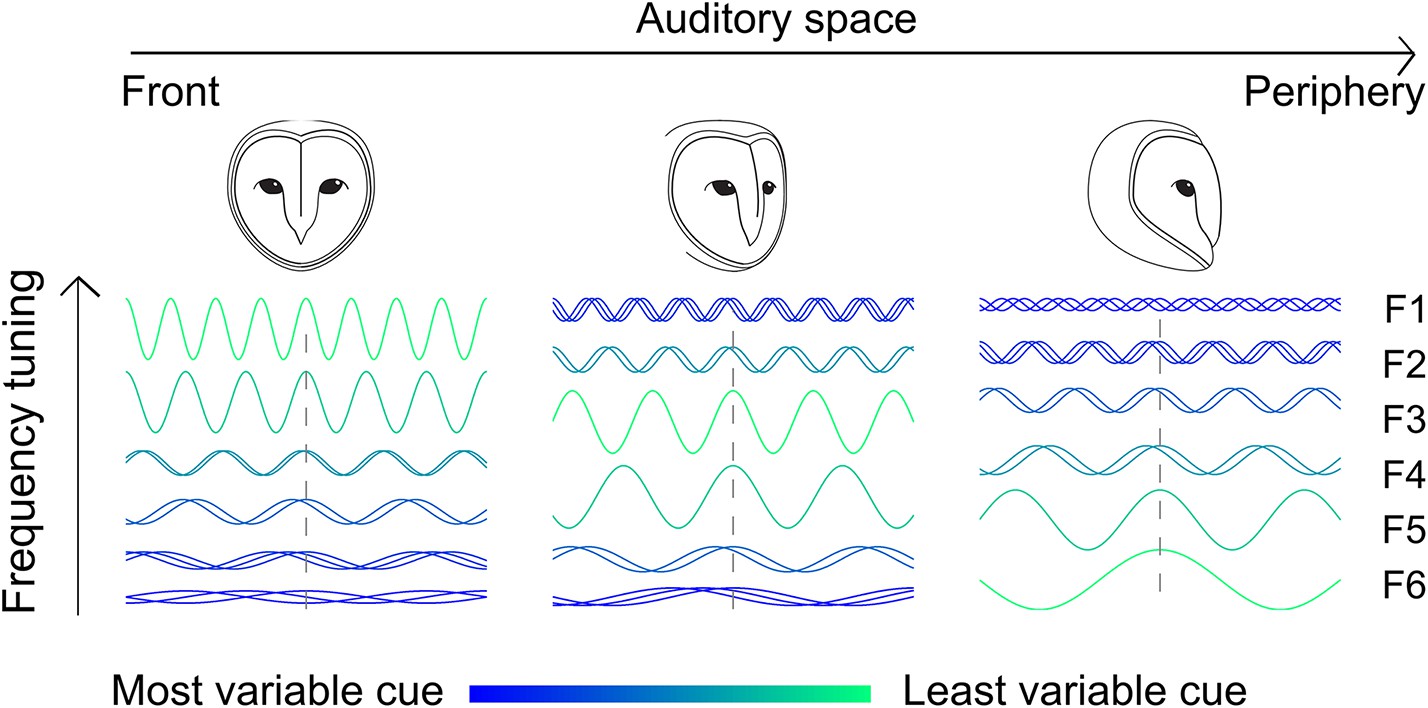
Adjusting tonotopy through weighting by reliability to represent space.
Neurons receive inputs where different frequencies (F1–F6) are weighted by the IPD variance. For neurons tuned to frontal space (left), a larger weight is assigned to high frequencies where IPD is less variable, while neurons tuned to more peripheral space (middle and right) receive stronger input at lower frequencies. The effect of the head on IPD variability is indicated by the color (green is less variable) and superimposed sine waves (superimposed sinusoids shifted in phase indicate more variability).
Author response image 1
Author response image 2
Download links
A two-part list of links to download the article, or parts of the article, in various formats.
Downloads (link to download the article as PDF)
Open citations (links to open the citations from this article in various online reference manager services)
Cite this article (links to download the citations from this article in formats compatible with various reference manager tools)
Spatial cue reliability drives frequency tuning in the barn Owl's midbrain
eLife 3:e04854.
https://doi.org/10.7554/eLife.04854


