Computations underlying Drosophila photo-taxis, odor-taxis, and multi-sensory integration
- New York University, United States
Figures
Figure 1
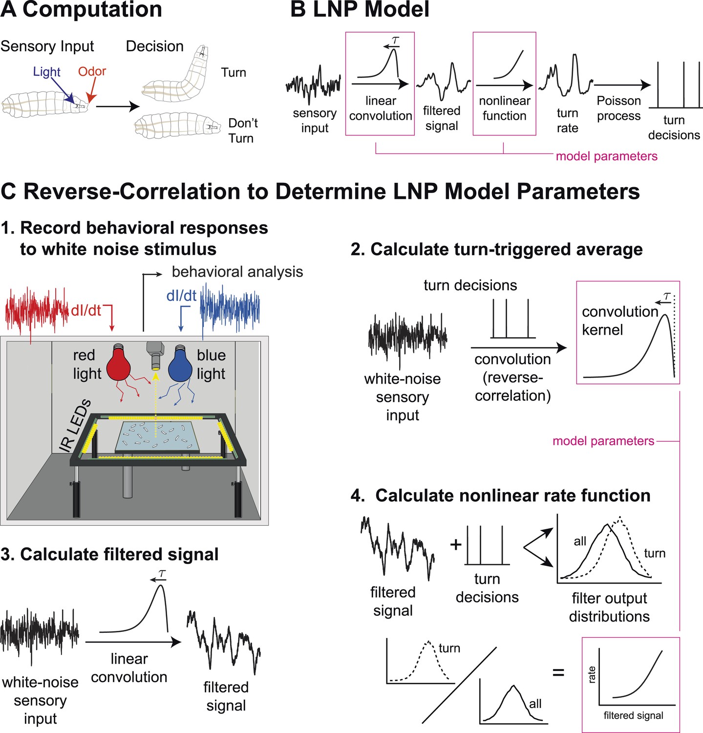
Identifying computations underlying the decision to initiate a turn.
(A) Computation: on the basis of sensory input (light or odor in this work) the larva decides whether or not to end a run and begin a turn. (B) LNP model of the computation: Sensory input is processed by a linear filter to produce an intermediate signal. The rate at which the larva initiates turns is a nonlinear function of this signal. Turns are initiated stochastically according to a Poisson process with this underlying turn rate. (C) Reverse-correlation to determine LNP parameters: (1) We presented groups of larvae with either blue or red light with randomly varying intensity derivatives. Blue light provided a visual stimulus, while red light activated CsChrimson expressed in sensory neurons. In multi-sensory experiments, uncorrelated red light and blue light signals were presented simultaneously. Larvae were observed under infrared illumination, and their behaviors were analyzed with machine vision software. (2) We calculated the ‘turn-triggered average’ (TTA) or the reverse-correlation between turn initiation and stimulus by averaging the stimulus that preceded each moment any larva initiated a turn. The TTA approximates the convolution kernel for the linear response of the LNP model. (3) Using the TTA as a convolution kernel and the known input signal, we computed the intermediate filtered signal. (4) Using the inferred filtered signal and the observed times at which turns were initiated, we found the nonlinear rate function by dividing the distribution of filtered signal values at the time of turn initiation (‘turn-triggered-ensemble’) by the distribution of all filtered signal values. Illustrations adapted from (Kane et al., 2013).
Figure 2 with 1 supplement
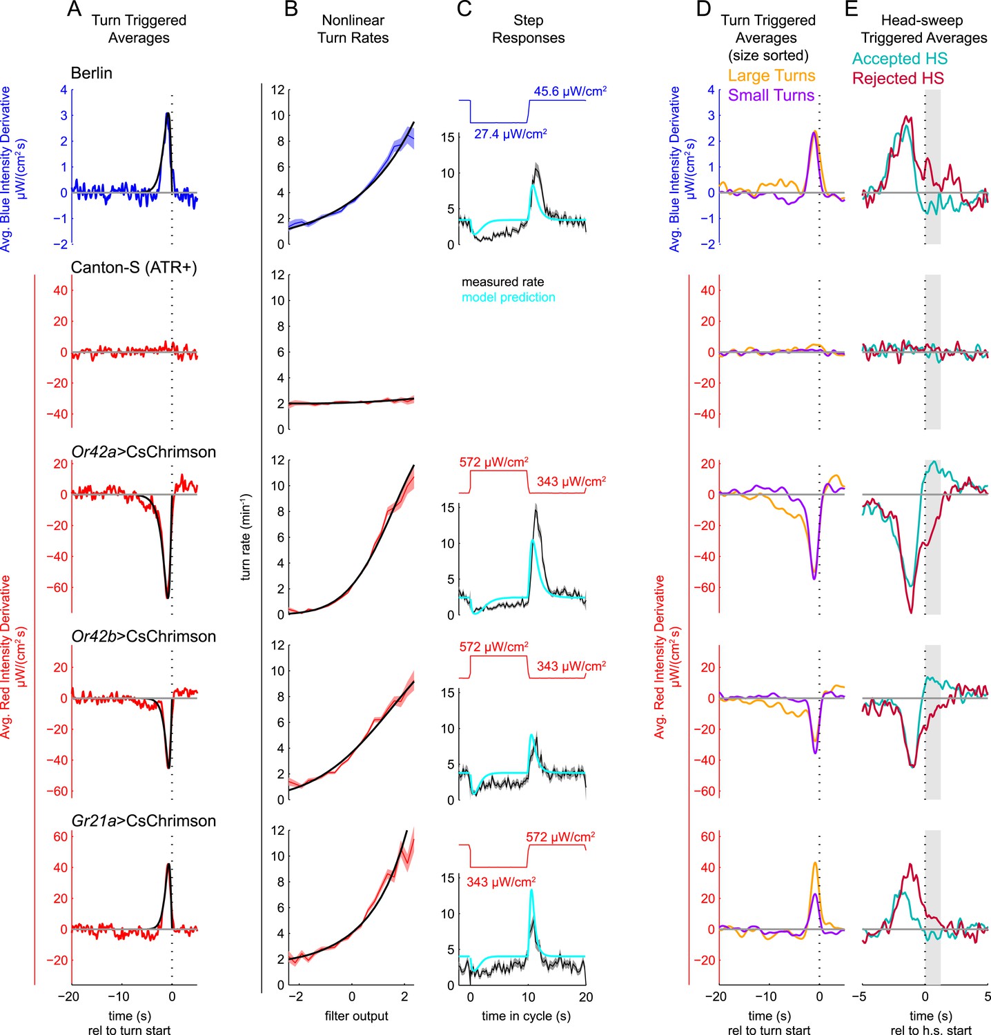
Unimodal reverse-correlation experiments.
Top row, Berlin wild-type larvae were stimulated with blue (λpeak = 448 nm; max intensity = 74 μW/cm2) light. All other rows, larvae of indicated genotype were stimulated with red light (λpeak = 655 nm; max intensity = 911 μW/cm2) while constant dim blue light (intensity = 3.7 μW/cm2) served as a visual mask. Column A: Turn triggered average. Average stimulus preceding (and following) each turn initiation. Turns are initiated at time 0 (indicated with dashed line). The black line is the smoothed TTA used as the linear filter. Column B: Measured turn rates as a function of calculated filter output. Line and shaded region represent mean turn rate and standard error due to counting statistics. Black line is the nonlinear turn rate modeled as a ratio-of-Gaussians (Pillow and Simoncelli, 2006). Column C: Step responses predicted by LNP model. Square waves of light with period 20 s and duty cycle 50% were presented to larvae. The LNP model was used to predict the resulting turn rates. Top graphs: light level vs time in cycle. A favorable change happens at t = 0 and an unfavorable change at t = 10 s. Bottom graphs: measured and predicted turn rates vs time in cycle. Black line and shaded region represent mean turn rate and standard error due to counting statistics. The cyan line is the exact prediction of the model using the parameters found from the corresponding reverse-correlation experiments. (A, B) The stimulus and analysis were cyclic, so the time range from −2 to 0 s is identical to that from 18–20 s. Column D: Size-sorted turn-triggered average. As in A, but turns were sorted into large (heading change during turn > rms heading change) and small turns. Displayed averages are lowpassed with a Gaussian filter (σ = 0.5 s) to clarify the long time-scale features. Column E: Head-sweep triggered average (for first head-sweep of turn). Average stimulus surrounding accepted (teal) and rejected (red) head-sweeps. Head sweeps were initiated at time t = 0 and concluded at a variable time in the future. The mean head-sweep duration (1.25 s) is indicated by the shaded region. See Table 1 for number of experiments, animals, and so on.
Figure 2—figure supplement 1
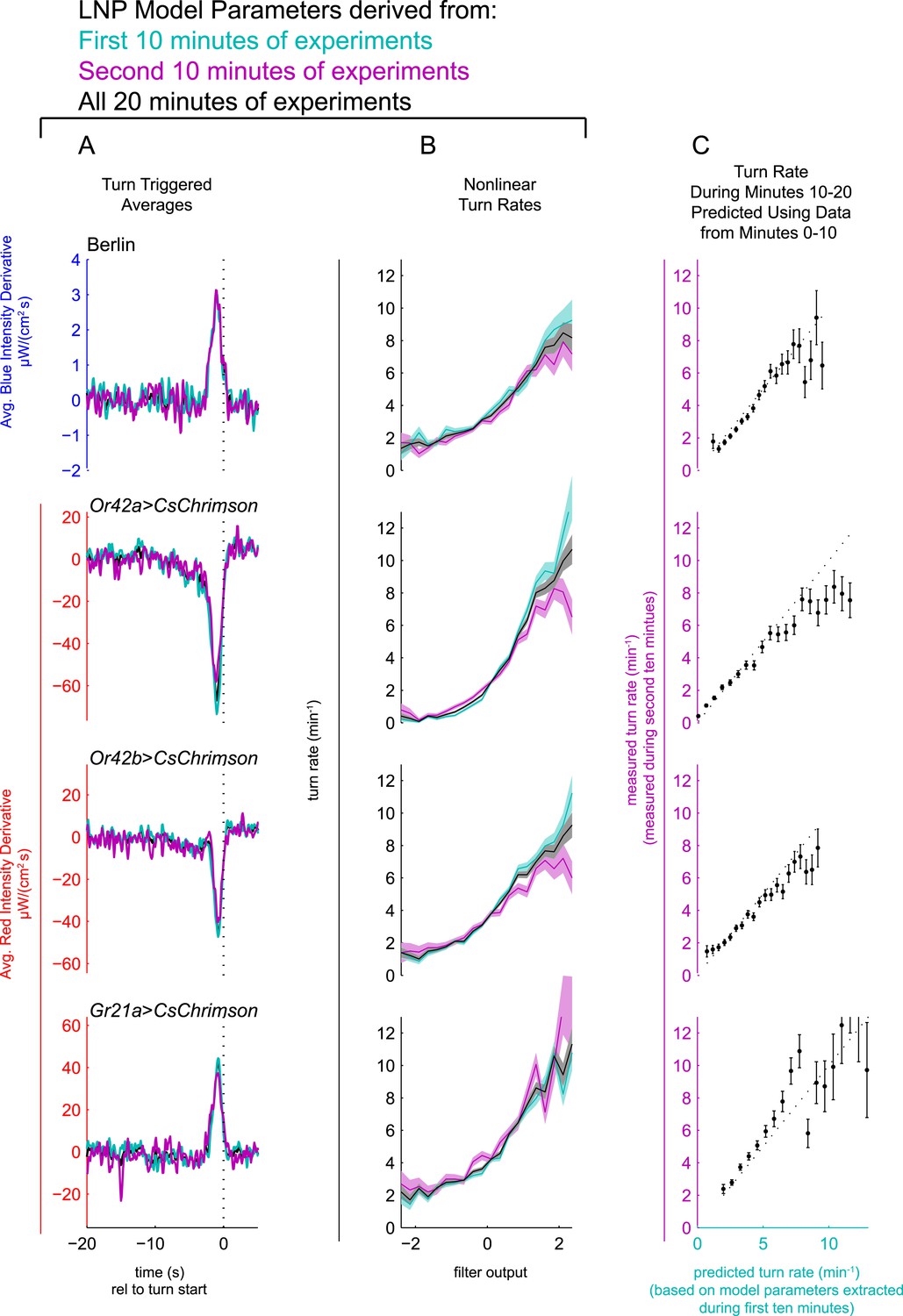
LNP model parameters are stable for duration of 20 min experiments.
Experiments of Figure 2 analyzed separately using data only from the first 10 min of experiment (teal) or only from the second 10 min of experiment (purple) or from entire 20 min data set (black). Column A: Turn triggered average. As in Figure 2A. The same convolution kernel is recovered from all three data sets. Column B: Measured turn-rates as a function of calculated filter output. As in Figure 2B. The turn rates vary across the three data sets mainly at high values of the filter output (stimulus conditions most likely to lead to turning). Column C: LNP model fits can predict response to white noise signals. Data from the first 10 min of the experiments were used to find LNP model parameters. The parameterized models were then used to predict the turn rate at each time point during the second 10 min of experiments. The measured turn rate during the second 10 min is plotted as a function of the model predictions. At high turn rates, for visual and fictive attractive odor stimuli, the turn rate is lower in the final 10 min than predicted by fits to the first 10 min, suggesting modest adaptation. For fictive CO2, the measured turn rate is higher than predicted, suggesting modest sensitization. Error bars represent the uncertainty due to counting statistics.
Figure 3 with 3 supplements
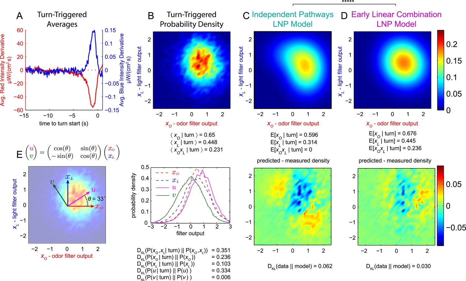
Multi-modal reverse-correlation experiments suggest attractive odor and light signals are combined linearly and early.
Or42a>CsChrimson larvae were presented with independently varying Brownian light intensities. Reverse-correlation analysis was carried out as in Figure 1. (A) TTA. Average change in red (fictive odor) and blue light intensities preceding turns. (B) Turn triggered ensemble. Top: 2D density histogram of calculated odor and light filter outputs at initiation of each turn. Bottom: 1D density histograms of filter outputs (xO,xL) and their linear combinations (u,v). DKL(P(x|turn)||P(x)) is the Kullback-Leibler divergence from the turn-triggered distribution to the distribution of x at all times. Larger values indicate that x carries more information about the decision to turn. (C, D) Predicted turn triggered ensemble according to, (C) independent pathways model and (D) early linear combination model. Top panel: predicted density. Bottom panel: difference between predicted density and measured density. DKL(data||model) is the Kullback-Leibler divergence of the model from the data; smaller values indicate a better match. ***** = P (Independent pathways model)/P (Early linear combination model) < 0.00001; Aikake Information Criterion Test. (E) Coordinate rotation described in text and used in bottom panel of B. Orthogonal coordinates (u,v) are rotated 33° relative to (xO,xL). Rotation is shown overlaid on turn-triggered probability density (B). See Table 1 for number of experiments, animals, and so on.
Figure 3—figure supplement 1

Graphical explanation of the independent pathways model.
https://doi.org/10.7554/eLife.06229.007
Figure 3—figure supplement 2
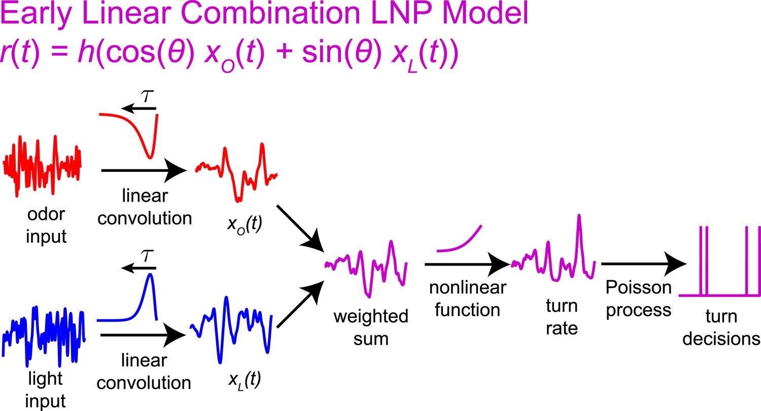
Graphical explanation of the early linear combination model.
https://doi.org/10.7554/eLife.06229.008
Figure 3—figure supplement 3

Visual and fictive olfactory stimuli do not cross-talk.
Larvae were presented with same red and blue Brownian light stimuli as in Figure 3. TTA of red and blue stimuli are shown on same axes as in Figure 3A. (A) Reproduced from Figure 3A: Larvae expressing CsChrimson in Or42a receptor neurons turn in response to increasing blue light and decreasing red light (fictive odor). (B) Genetically blinded larvae expressing CsChrimson in Or42a receptor neurons turn in response to decreasing red light (fictive odor) but are unresponsive to blue light. (C) Wild-type larvae not expressing CsChrimson turn in response to increasing blue light but are unresponsive to red light. See Table 1 for number of experiments, animals, and so on.
Figure 4
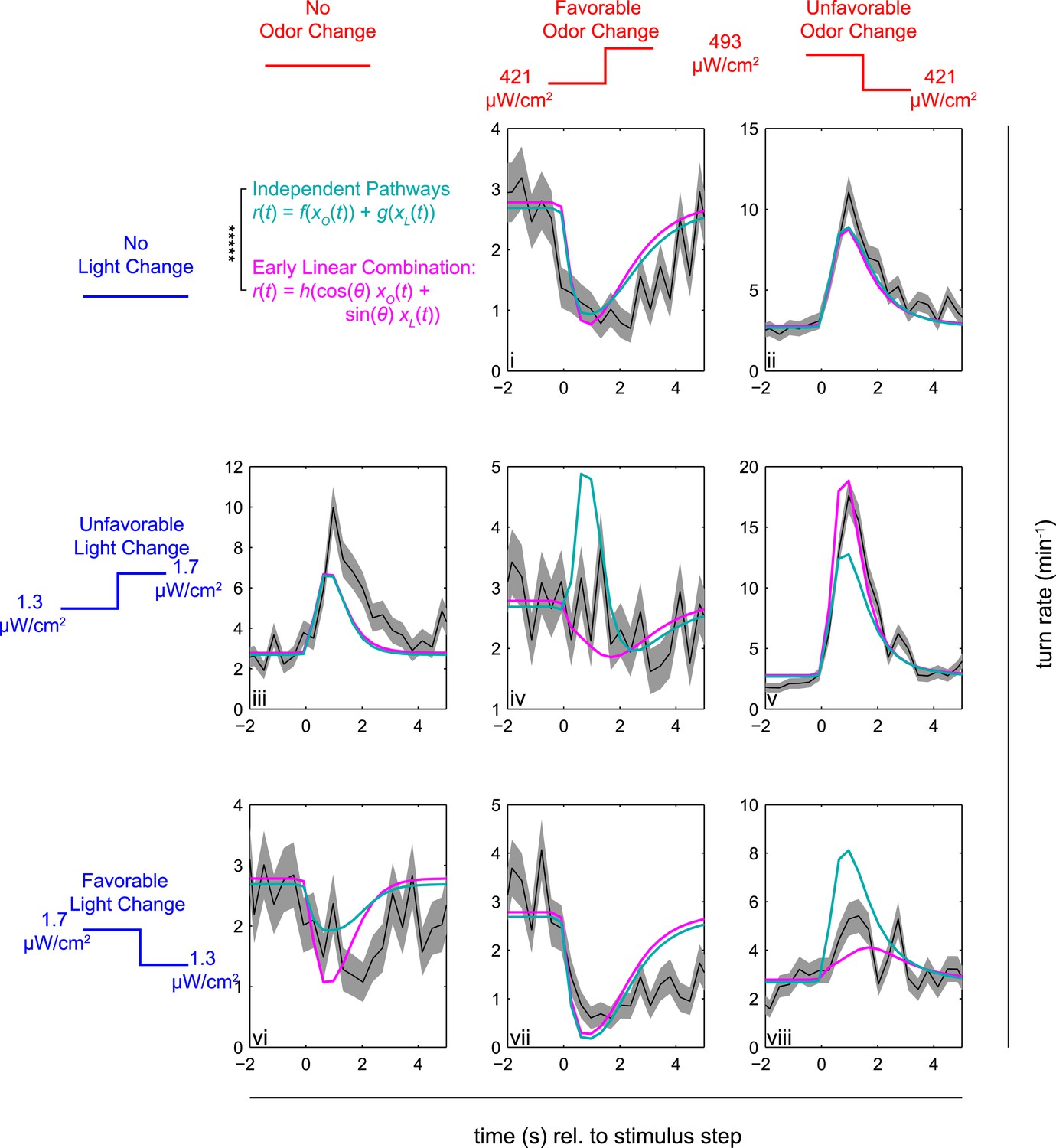
Multi-modal step responses support early linear combination of odor and light signals.
Turn rates vs time for Or42a>CsChrimson larvae responding to coordinated increases and decreases of red and blue light. All steps occur at t = 0. Left column: no change in fictive odor, center column: red light increases at t = 0 right column: red light decreases at t = 0. Top row: no change in visual stimulus, center row: blue light increases at t = 0, bottom row: blue light decreases at t = 0. For instance, in panel iii blue light increased at time 0, while red light remained constant; in iv, both red and blue light increased at time 0; and in v, blue light increased and red light decreased at time 0. Black line and shaded region represent mean turn rate and standard error due to counting statistics. Cyan line is the best-fit (maximum likelihood estimate, 6 parameter fit) prediction of the independent pathways model. Magenta line is the best-fit (maximum likelihood estimate, 4 parameter fit) prediction of the early linear combination model. Note that the time axis is the same for each subplot, but the turn rate axis varies. ***** = P (Independent pathways model)/P (Early linear combination model) < 0.00001; Aikake Information Criterion Test, measured for the entire data set. See Table 1 for number of experiments, animals, and so on.
Figure 5
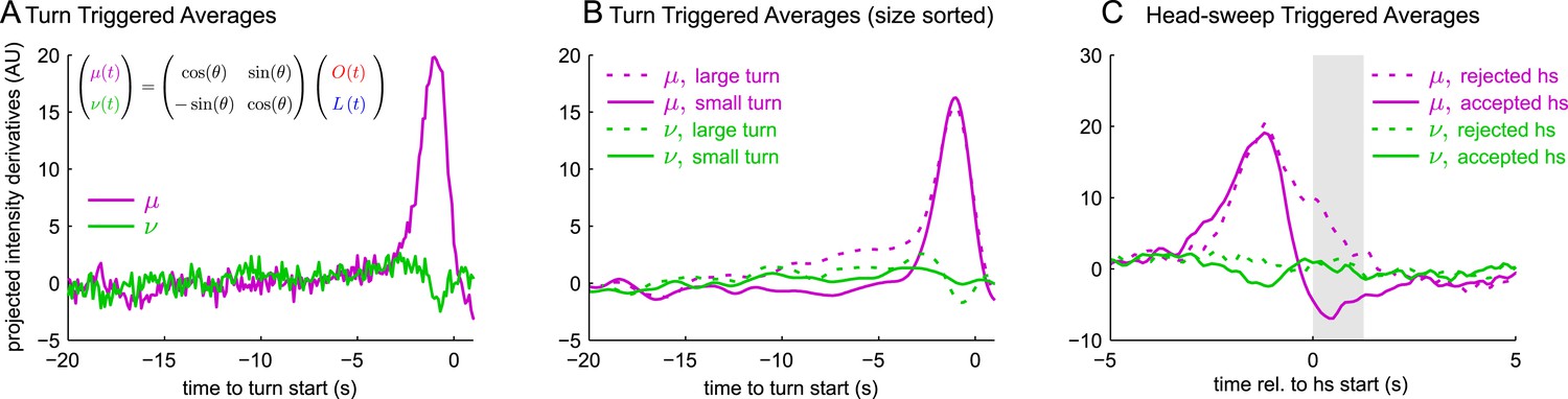
All navigational decisions appear to be based on a single linear combination of odor and light inputs.
(A–C) Reverse correlation in rotated coordinate system. μ,ν are linear combinations of the raw input stimuli according to the same scaling as used to combine filtered odor and light signals in Figure 3. (A) Turn-triggered averages. Average change in μ,ν prior to start of a turn. (B) Size-sorted turn-triggered averages. Displayed averages are lowpassed with a Gaussian filter (σ = 0.5 s) to clarify the long time-scale features. (C) Head-sweep-triggered average (for first head-sweep of turn). Shaded region indicates mean head-sweep duration (1.25 s).
Figure 6
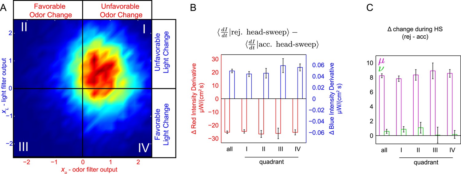
Probing for attentional shifts during multi-modal noise experiments.
(A) Turn-triggered ensemble (duplicated from Figure 3B), with quadrants highlighted. Color scale the same as in 3B. Quadrants I–IV indicate which stimulus or stimuli likely provoked the larva to turn (I—both odor and light stimulated turning; II—light, but not odor, stimulated turning; III—neither odor nor light were changing unfavorably; IV—odor, but not light, stimulated turning). Each turn was assigned to one of these quadrants based on the filtered signal values (xO,xL) at the time the turn started. (B, C) Difference in intensity changes during accepted and rejected head sweeps (first head-sweep of turn only). Difference in mean rate of change in intensity over mean head sweep duration (1.25 s, shaded region in 5C) between rejected and accepted head-sweeps. Error bars are ±1 s.e.m. (B) Changes in odor and light intensities. (C) Changes in rotated coordinate system. See Table 1 for number of experiments, animals, and so on.
Videos
Video 1
Calculating the turn-triggered average.
Left panel: annotated video image of individual larva. Thin white line: larva's path (past and future). Gold dots: markers along midline of animal, used to determine posture. Upper left corner: time (since experiment start) and behavioral state. Right panels: top: light derivative (AU) vs. time; current time is indicated by dashed cyan line. Middle panels: speed and body bend angle, metrics used to determine behavioral state, vs. time. Shading indicates behavioral state (blue = run, white = turn; within turns, red = rejected head sweep, green = accepted head sweep). Current time is indicated by cyan dot. Bottom panel: turn-triggered average light (TTA) intensity derivative (AU), calculated based on turns preceding the one shown. Animation: The time preceding and following individual turns is featured. At the moment a larva initiates a turn, we ‘grab’ the sequence of light intensity derivatives and add it to a running average (shown at the bottom). As we include more turns in the average (number of included turns is indicated by ‘turn #’ above the left panel—note logarithmic spacing of turn #s), we build up a ‘TTA’ that approximates the linear filter in the LNP model.
Tables
Table 1
Numbers of experiments, animals, turns, and head sweeps for all figures
| Genotype | #expts | #animals | hours | #turns | rms turn size | #large turns | #small turns | #accepted head sweeps | #rejected head sweeps |
|---|---|---|---|---|---|---|---|---|---|
| Uni-modal reverse-correlation experiments (Figure 2A,B,D,E, Figure 2—figure supplement 1) | |||||||||
| Berlin | 6 | 150 | 52.6 | 6594 | 76.4 | 2462 | 4132 | 4139 | 2455 |
| Canton-S | 7 | 334 | 117.7 | 8824 | 66.0 | 3086 | 5738 | 5570 | 3254 |
| Or42a>CsChrimson | 5 | 180 | 61.1 | 6971 | 68.9 | 2531 | 4440 | 4122 | 2849 |
| Or42b>CsChrimson | 6 | 246 | 64.4 | 9565 | 73.3 | 3480 | 6085 | 6215 | 3350 |
| Gr21a>CsChrimson | 5 | 227 | 54.2 | 8760 | 75.1 | 3392 | 5368 | 5424 | 3336 |
| Uni-modal step experiments (Figure 2C) | |||||||||
| Berlin | 4 | 95 | 34.7 | 3674 | – | – | – | – | – |
| Or42a>CsChrimson | 2 | 107 | 36.6 | 3905 | – | – | – | – | – |
| Or42b>CsChrimson | 2 | 99 | 21.5 | 2599 | – | – | – | – | – |
| Gr21a>CsChrimson | 2 | 111 | 22.1 | 2384 | – | – | – | – | – |
| Multi-modal reverse-correlation experiments (Figure 3, 5, 6, Figure 3—figure supplement 3) | |||||||||
| Or42a>CsChrimson | 12 | 608 | 136 | 21,075 | 66.6 | 7225 | 13,850 | 12,795 | 8280 |
| quadrant I | – | – | – | 10,363 | – | – | – | 6216 | 4147 |
| quadrant II | – | – | – | 3301 | – | – | – | 2086 | 1215 |
| quadrant III | – | – | – | 1684 | – | – | – | 1088 | 596 |
| quadrant IV | – | – | – | 5727 | – | – | – | 3405 | 2322 |
| GMR-Hid, Or42a>CsChrimson | 3 | 121 | 28.9 | 4842 | – | – | – | – | – |
| Canton-S | 3 | 166 | 39.9 | 3412 | – | – | – | – | – |
| Multi-modal step experiments (Figure 4) | |||||||||
| Or42a>CsChrimson | 5 | 250 | 50 | 7859 | – | – | – | – | – |
-
#expts: Number of 20 min experiments. For reverse-correlation experiments, each experiment presented a different stimulus sequence with the same statistical properties; for step experiments, the same stimulus pattern was presented in each experiment.
-
#animals: Approximate number of animals, taken by finding the maximum number of animals tracked in a 30-s window during each experiment.
-
#hours: total observation time in units of larva-hours. Observing 3 larvae for 20 min each would equal 1 larva-hour.
-
#turns: total number of turns observed and used in analysis.
-
rms turn size: root mean square turn size in degrees (defined as angular difference in run heading immediately before and after a turn) for the set of experiments.
-
#large/small turns: number of turns with angular changes larger/smaller than the rms turn size.
-
#accepted head sweeps: number of times the first head sweep of a turn was accepted, ending in a new run.
-
#rejected head sweeps: number of times the first head sweep of a turn was rejected, leading to another head sweep.
Table 2
Kullback-Leibler divergences for Figure 3
| KL divergence | k-NN | model data as normally distributed | Szegö-PSD method |
|---|---|---|---|
| Figure 3B: | 0.351 | 0.325 | – |
| Figure 3B: | 0.236 | 0.223 | 0.235 |
| Figure 3B: | 0.103 | 0.100 | 0.104 |
| Figure 3B: | 0.334 | 0.324 | 0.333 |
| Figure 3B: | 0.006 | 0.0002 | 0.003 |
| Figure 3C: | 0.062 | 0.035 | – |
| Figure 3D: | 0.030 | 0.007 | – |
-
KL divergence: the divergence to be calculated. k-NN: divergence calculated using the k-nearest neighbors algorithm. This value is displayed in Figure 3. model data as normal distributed: the distributions are modeled as Gaussians, whose divergence is calculated analytically. Szegö-PSD method: divergence between 1D distributions calculated by an alternate method.
Download links
A two-part list of links to download the article, or parts of the article, in various formats.
Downloads (link to download the article as PDF)
Open citations (links to open the citations from this article in various online reference manager services)
Cite this article (links to download the citations from this article in formats compatible with various reference manager tools)
Computations underlying Drosophila photo-taxis, odor-taxis, and multi-sensory integration
eLife 4:e06229.
https://doi.org/10.7554/eLife.06229


