Extracellular space preservation aids the connectomic analysis of neural circuits
- National Institutes of Health, United States
- University of Maryland, United States
- Max Planck Institute for Medical Research, Germany
Figures
Figure 1 with 2 supplements

ECS preservation in acutely isolated tissues.
(A) A model of the changes brain tissue undergoes during chemical tissue fixation and possible interventions to preserve ECS. (B) ECS fraction of mouse olfactory bulb (x), retina (o), and cortex (□) correlates with increasing fixative vehicle concentration. Dashed line is the linear fit to olfactory bulb data, solid line is the linear fit to cortex data (olfactory bulb: R = 0.80, p = 0.0006; cortex: R = 0.79, p = 0.0113). (C–F) EM images from the external plexiform layer of the mouse olfactory bulb from a perfused brain (C) or from acute sections fixed with increasing buffer concentrations (D–F). ECS fractions are 0.6% (C), 5.8% (D), 11.3% (E), and 23.9% (F). Scale bars: 1 µm (C–F). ECS: Extracellular space; EM: Electron microscopy.
Figure 1—figure supplement 1

Change of tissue dimensions and uniformity of ECS preserved sections.
(A) Vibratome sections were cut from the cerebral cortex of acutely isolated brains (for ECS preservation) or from perfused animals. Section thickness was nominally 500 µm as determined by the slice thickness setting of the vibratome. Sections were stained for EM and the cross-sectional thickness measured from EM images (mean +/- SEM; n = 20 slices from 6 animals, one-way ANOVA: p = 0.46). (B) Sample images from the edges (Bi, Biii) and center (Bii) of a 500-µm-thick section of the mouse olfactory bulb. ECS is evenly preserved across the section. ECS: Extracellular space; EM: Electron microscopy.
Figure 1—figure supplement 2
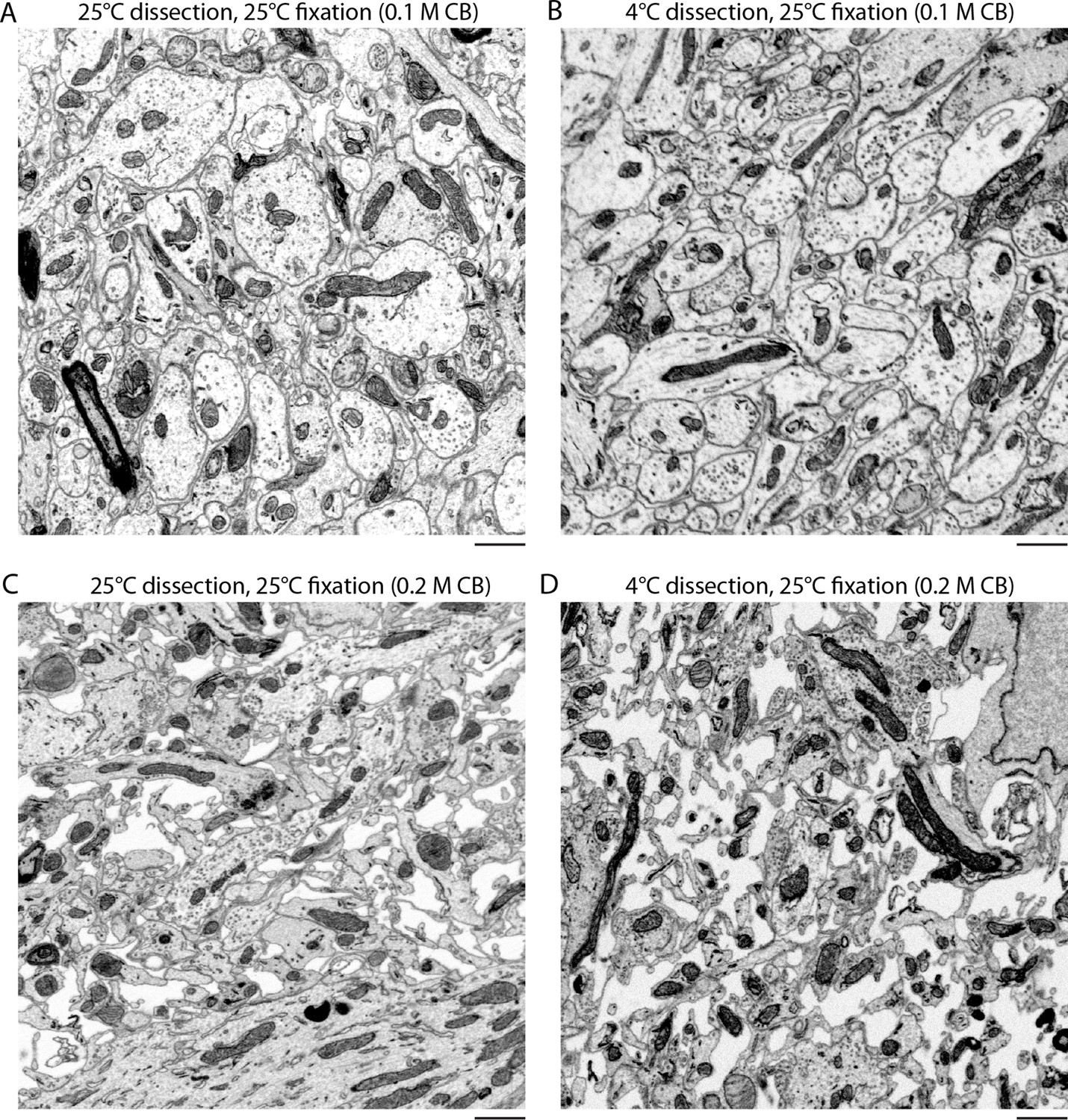
Effect of temperature on the preservation of ECS.
(A,B) Vibratome sections were cut from the olfactory bulbs of acutely isolated brains at either 4°C or 25°C and then fixed at 25°C in 0.1 M CB + 2% GA. (C,D) Vibratome sections were cut from the olfactory bulbs of acutely isolated brains at either 4°C or 25°C and then fixed at 25°C in 0.2 M CB + 2% GA. ECS preservation was similar under both conditions indicating the temperature of solutions during tissue dissection is not a major determinant for ECS preservation. Scale bars: 1 μm. ECS: Extracellular space; EM: Electron microscopy.
Figure 2 with 1 supplement
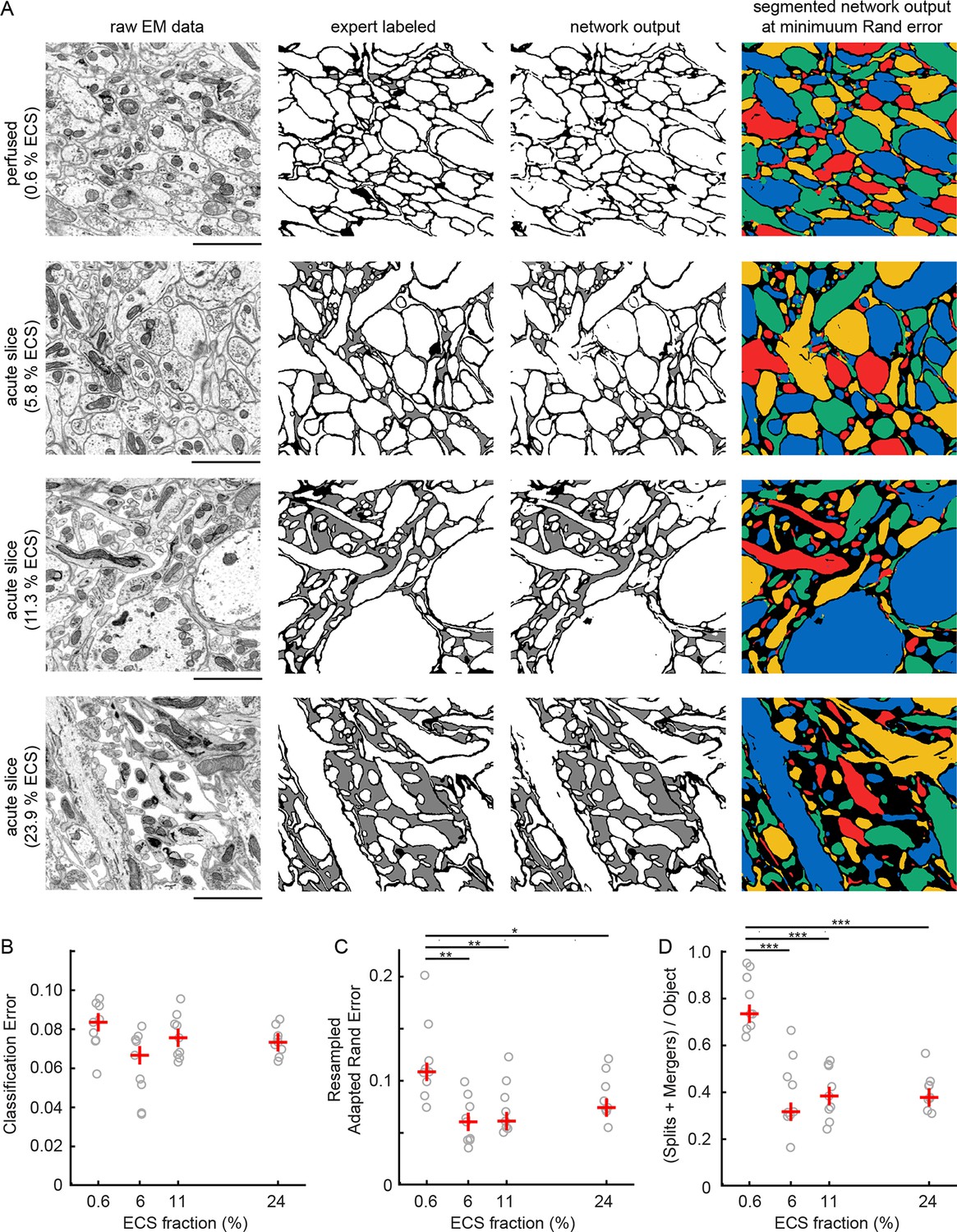
Automated 2D segmentation of extracellular space preserved data.
(A) Four raw EM images (first column) of varying ECS fractions (0.6, 5.8, 11.3, and 23.9%) were analyzed. The lowest ECS fraction (0.6%) is the perfused preparation while the others are the acute slice preparations. Pixels in each image were annotated (second column) as either intracellular (white), extracellular (gray), or plasma membrane (black). Representative test image pixel classifications (third column) yielded network classification errors of 9.3, 8.1, 6.7, and 7.2% for the four examples shown. Intracellular pixel probabilities were thresholded and segmented (fourth column) to yield minimum Rand errors of 0.11, 0.06, 0.06, and 0.07 for the four examples shown. (B) Pixel classification errors plotted versus ECS fraction from an ninefold cross-validation, median values in red, shows no significant difference between perfused and acute preparations (K-W test: p=0.05). (C) Rand error plotted versus ECS fraction for the ninefold cross-validation, median values in red, shows a significant difference between perfused and acute preparations (K-W test: p<0.01; Wilcoxon rank-sum test: p=0.0017 [5.8%], p=0.0091 [11.3%], p=0.031 [23.9%]). (D) Total number of splits and merger per object in each test image plotted versus ECS fraction for the ninefold cross-validation, median values in red, shows a significant difference between perfused and acute preparations (K-W test: p<0.001; Wilcoxon rank-sum test: p=0.00049 [5.8%], p=0.00035 [11.3%], p=0.00035 [23.9%]). Scale bars: 2 μm. p-Values: *p<0.05, **p<0.01, ***p<0.001. ECS: Extracellular space; EM: Electron microscopy.
-
Figure 2—source data 1
Raw image and expert labels of 0.6% ECS data.
TIFF stack viewable using ImageJ. ECS: Extracellular space.
- https://doi.org/10.7554/eLife.08206.007
-
Figure 2—source data 2
Raw image and expert labels of 5.8% ECS data.
TIFF stack viewable using ImageJ. ECS: Extracellular space.
- https://doi.org/10.7554/eLife.08206.008
-
Figure 2—source data 3
Raw image and expert labels of 11.3% ECS data.
TIFF stack viewable using ImageJ. ECS: Extracellular space.
- https://doi.org/10.7554/eLife.08206.009
-
Figure 2—source data 4
Raw image and expert labels of 23.9% ECS data.
TIFF stack viewable using ImageJ. ECS: Extracellular space.
- https://doi.org/10.7554/eLife.08206.010
Figure 2—figure supplement 1
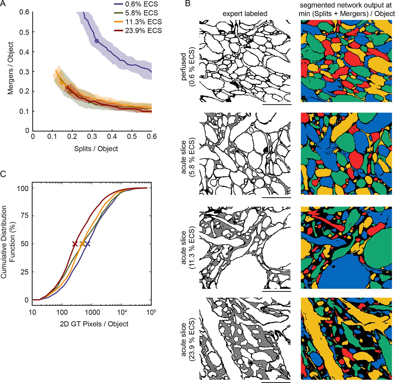
Warping error of automated segmentations.
(A) Split/merger curves parameterized by threshold of the network output. Shaded area is the standard error of the mean, lines are the mean number of splits/mergers per object, and the circles are the mean of the minimum total splits + mergers per object. (B) Network segmentations at the minimum warping error threshold, same regions as in Figure 2A. Warping errors were 0.68 (0.6% ECS), 0.32 (5.8% ECS), 0.52 (11.3% ECS), and 0.56 (23.9% ECS) for the four examples shown. (C) Cumulative distributions of the number of ground truth intracellular pixels per object for the four datasets. The difference in these distributions motivated the use of a Bernoulli sampling procedure for calculating the adapted Rand Error metrics in Figure 2C. Scale bars: 2 μm. ECS: Extracellular space.
Figure 3 with 1 supplement
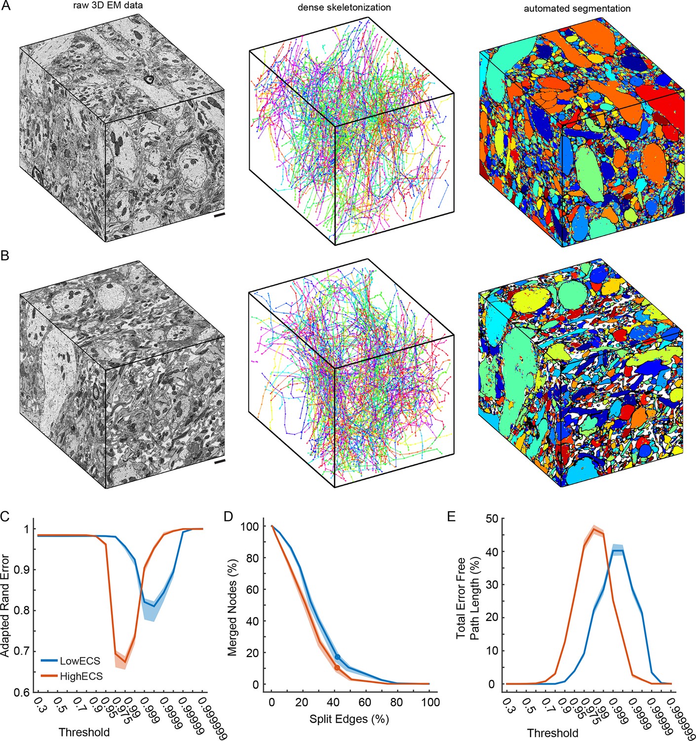
Automated 3D segmentation of extracellular space preserved data.
(A) A 10 x 10 x 12 μm3 3D SBEM cube (left) of perfused tissue (LowECS), a dense skeletonization of all neurites in the volume (middle), and an automated segmentation of the volume (right). (B) A 10 x 10 x 12 μm3 3D SBEM cube (left) of ECS-preserved tissue (HighECS), a dense skeletonization of all neurites in the volume (middle), and an automated segmentation of the volume (right). (C) Adapted Rand error of automated segmentations compared to dense skeletonizations as a function of the segmentation threshold for the HighECS (brown) and LowECS (blue) data volumes. (D) The fraction of merged skeleton nodes versus split skeleton edges as a function of network threshold. Solid points indicate the minimum sum of the error fractions. (E) The total error-free skeleton path length recovered as a function of network threshold. Shaded regions in C–E are the 99% confidence intervals based on a Bernoulli sampling of the data. Scale bars in A, B = 1 μm. SBEM: Serial block-face scanning electron microscopy.
-
Figure 3—source data 1
M0027_11 dense skeletonization, Knossos NML file.
- https://doi.org/10.7554/eLife.08206.013
-
Figure 3—source data 2
M0007_33 dense skeletonization, Knossos NML file.
- https://doi.org/10.7554/eLife.08206.014
-
Figure 3—source data 3
M0007_33 training data cubes.
- https://doi.org/10.7554/eLife.08206.015
-
Figure 3—source data 4
M0027_11 training data cubes.
- https://doi.org/10.7554/eLife.08206.016
Figure 3—figure supplement 1
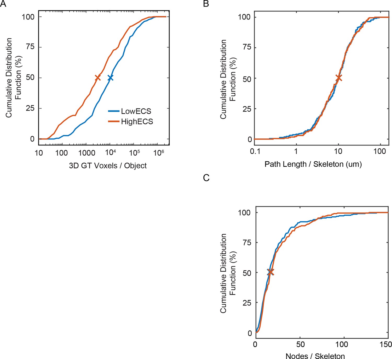
Cumulative distributions for 3D hand-labeled volumes and skeletonizations of the LowECS (blue) and HighECS (brown) data volumes.
(A) Cumulative distribution frequency (CDF) of number of intracellular ground truth voxels per object. The distribution medians are significantly different (Wilcoxon rank-sum test, p <0.0001). (B) CDF of path length per skeleton, medians 10.2 (LowECS) and 10.1 (HighECS) μm. The distributions are not significantly different (two-sample Kolmogorov–Smirnov (KS) test, p = 0.91). (C) CDF of the number of nodes annotated per skeleton, medians 16 (LowECS) and 17 (HighECS) nodes. The distributions not significantly different (two-sample KS test, p = 0.77).
Figure 4 with 1 supplement
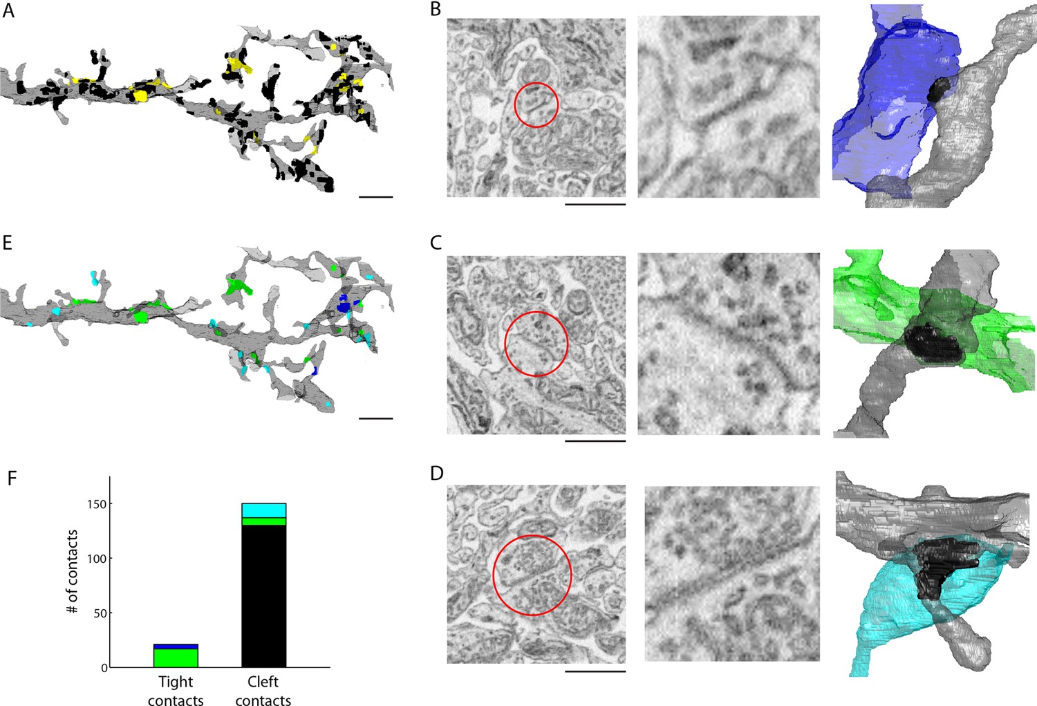
Extracellular space aids the identification of gap junctions.
(A) Reconstructed dendrites of an AII amacrine cell (gray) and surface renderings of tight (yellow) and cleft (black) contacts. (B-D) Example EM images and volumetric reconstructions of (B) an AII (gray) to AII (blue) tight contact, (C) an AII (gray) to cone bipolar cell (green) tight contact (C), and (D) a cleft contact identified as a chemical synapse between a presynaptic amacrine cell (cyan) and the AII cell (gray). (E) Tight contact surface renderings color-coded by the identity of the synaptic partner: AII amacrine cell (blue), cone bipolar cell (green), presynaptic amacrine cell (cyan). (F) Summary of the number of contacts color-coded by the cell type of the contacting cell: AII (blue), cone bipolar (green), presynaptic amacrine cell (cyan), other (black). Scale bars: 2 µm (A,E), 1 µm (B–D). EM: Electron microscopy.
-
Figure 4—source data 1
Example image stack of an A2 to A2 tight contact.
TIFF stack viewable using ImageJ. Slice #128 in the stack indicates the location of the tight contact.
- https://doi.org/10.7554/eLife.08206.019
-
Figure 4—source data 2
Example image stack of a cone bipolar to A2 tight contact.
TIFF stack viewable using ImageJ. Slice #128 in the stack indicates the location of the tight contact.
- https://doi.org/10.7554/eLife.08206.020
-
Figure 4—source data 3
Example image stack of a chemical synapse to A2 cleft contact.
TIFF stack viewable using ImageJ. Slice #128 in the stack indicates the location of the cleft contact.
- https://doi.org/10.7554/eLife.08206.021
Figure 4—figure supplement 1
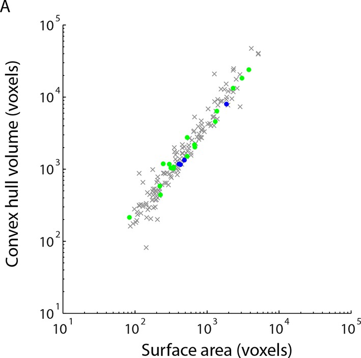
Simple measures of contact geometry do not predict gap junctions.
(A) Surface area and the volume of the convex hull bounding each contact are plotted for cleft contacts (gray), AII amacrine cell tight contacts (blue) and cone bipolar cell tight contacts (green).
Figure 5

Extracellular space preservation increases access to antibodies.
(A) Flat-mounted retinas were immunolabeled for vACHT with and without ECS preservation. Retinas were then cross-sectioned and confocal images were taken to directly visualize penetration depth. (B) Same as A, but immunolabeled for vGAT. (C) Fullwidth half-maximal penetration distances (mean +/- SEM) for retinas with and without ECS preservation (n = 20 retina slices from two animals, unpaired Student’s t-test, vACHT: ***p<0.0001, vGAT: ***p<0.0001). (D) EM images collected from the regions of interest in panel B indicated by dotted rectangles. Scale bars: 50 μm (A,B), 1 μm (D).
Download links
A two-part list of links to download the article, or parts of the article, in various formats.
Downloads (link to download the article as PDF)
Open citations (links to open the citations from this article in various online reference manager services)
Cite this article (links to download the citations from this article in formats compatible with various reference manager tools)
Extracellular space preservation aids the connectomic analysis of neural circuits
eLife 4:e08206.
https://doi.org/10.7554/eLife.08206


