A central role for the retrosplenial cortex in de novo environmental learning
- University College London, United Kingdom
Figures
Figure 1

The virtual reality environment ‘Fog World’.
(A) Examples of the ‘alien’ landmarks. (B) Landmarks positioned within the virtual world. (C) An overhead perspective of the environment showing the five different coloured, intersecting paths—note this aerial view was never seen by participants during learning.
Figure 2
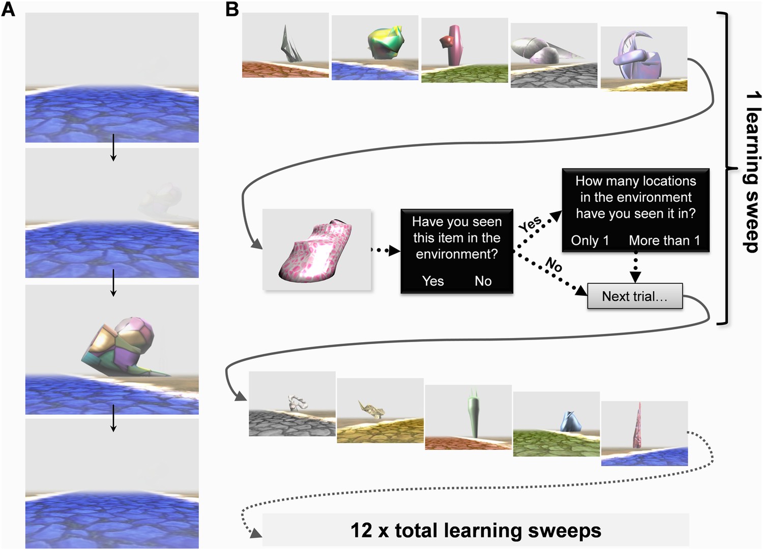
The Experimental paradigm.
While undergoing functional MRI (fMRI) scanning, subjects were presented with videos travelling along the various paths. (A) An example sequence of video frames with a landmark emerging through the fog, the camera turning towards it before returning back to the middle of the path—see also Video 1. (B) After viewing videos of each of the five paths once, subjects answered a series of questions about individual landmarks to test their learning throughout the experiment. A learning ‘sweep’ consisted of one round of videos of the five paths and the questioning period which followed. There were 12 learning sweeps.
Figure 3
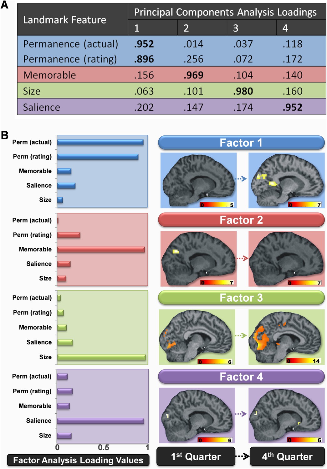
Changes in the brain regions engaged by different landmark features over the course of learning.
(A) The loading values of each landmark feature to the four principal component factors. Values above 0.5 are highlighted in bold. Factor 1 was strongly related to landmark permanence, factor 2 to their memorableness, factor 3 to their size and factor 4 to the visual salience of landmarks. (B) The bar graphs to the left show how strongly each of the four factors was related to the various features rated by subjects in the post-scan debrief. The associated brain regions responding to these four factors in the first and last quarters of learning are shown to the right. All activations are shown on a structural MRI brain scan of single representative subject. Each factor's activations are shown on the same sagittal slice and using a whole brain uncorrected threshold of p < 0.00001 for display purposes. The colour bars indicate the Z-score associated with each voxel.
Figure 4
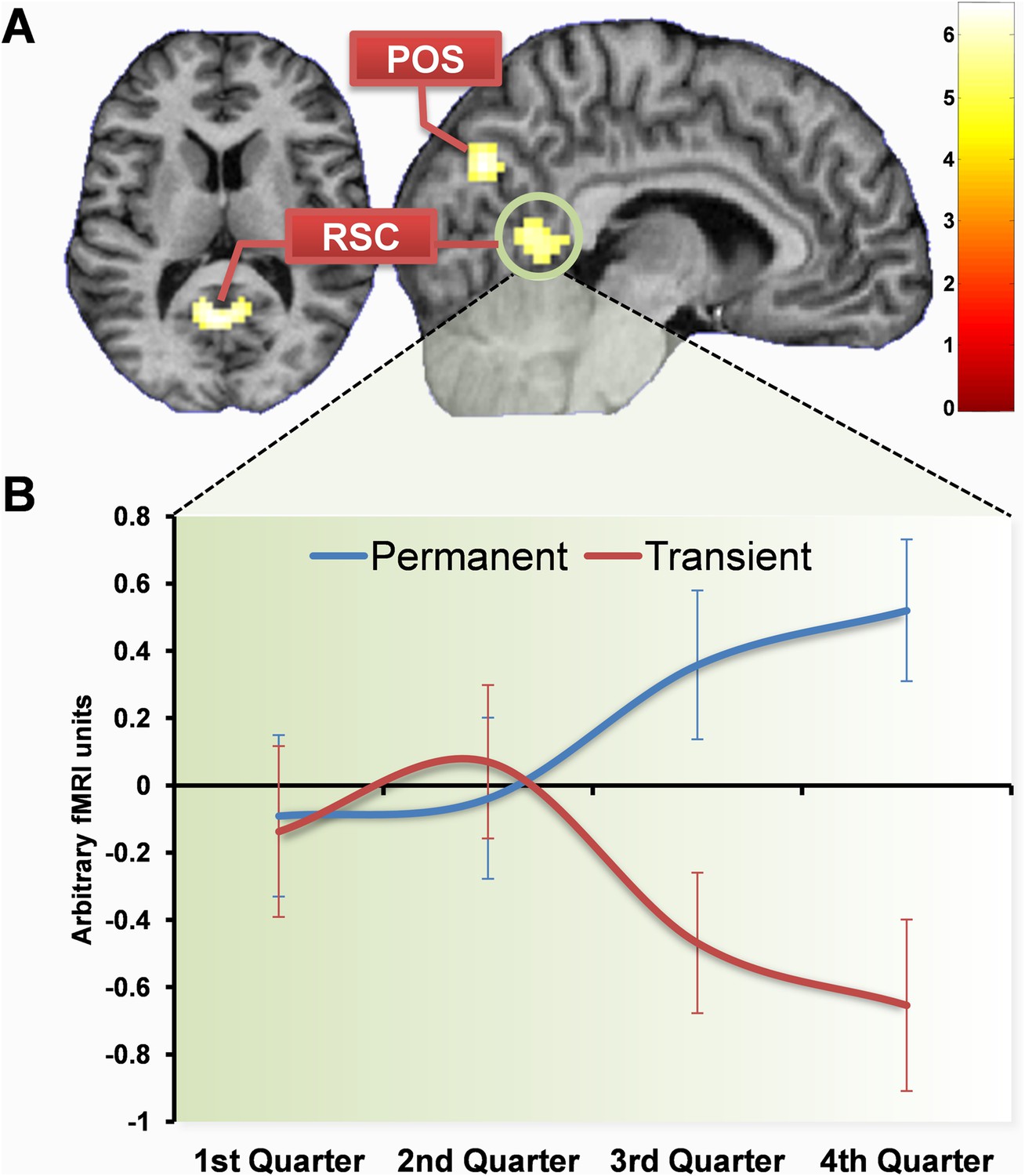
Brain regions more engaged by permanent than transient landmarks by the end of learning.
(A) Shows activations in retrosplenial cortex (RSC) and posterior parieto-occipital sulcus (POS) at the default threshold of p < 0.05 (FWE). The colour bar indicates Z-score associated with each voxel. (B) Shows a plot of mean blood oxygenation level-dependent (BOLD) responses (±1 SEM) within the RSC cluster (circled in green). In the first two quarters of scanning, responses to permanent (blue) and transient (red) landmarks did not differ, but as subjects learned landmark permanence, BOLD responses increased for permanent landmarks with a corresponding decrease for transient landmarks.
Figure 5
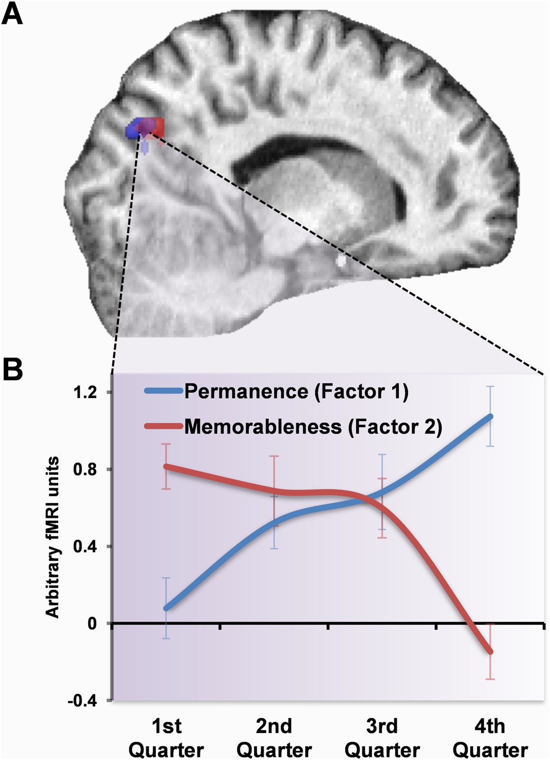
Response profile in POS.
(A) POS responded to memorable landmarks (those with higher factor 2 values) in the first quarter of learning (red) and permanent ones (with higher values for factor 1) in the final quarter (blue). The overlap of these activations is shown in purple. (B) The response profile of the overlapping (purple) voxels for the two factors throughout whole scan. Responses were initially greater for memorable landmarks but then switched over the course of learning to eventually become responsive to permanence. Plots show mean BOLD responses ±1 SEM. Activations are shown on a structural MRI brain scan of single representative subject at the default threshold of p < 0.05 (FWE).
Figure 6
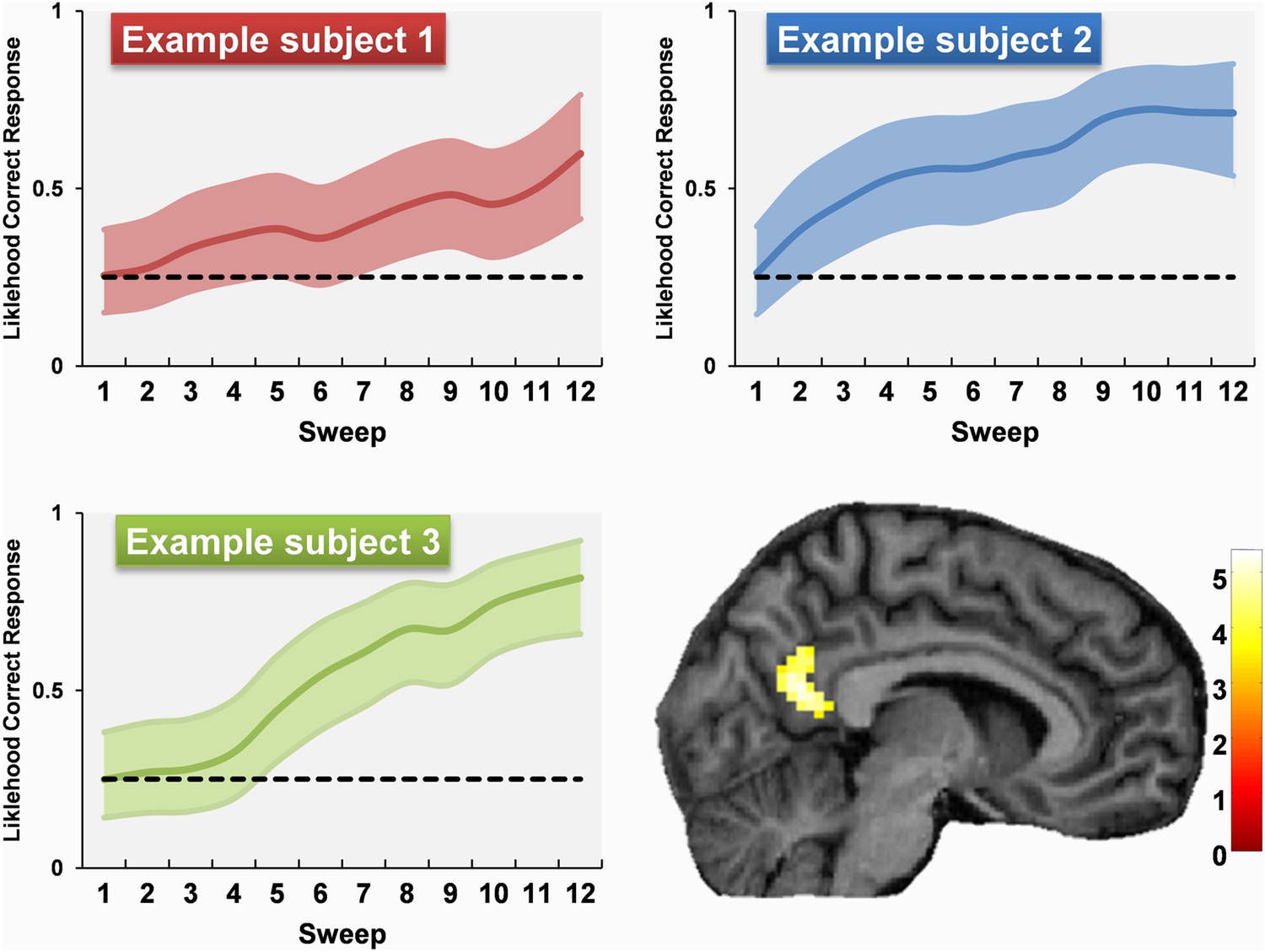
Examples of permanence learning curves and the associated fMRI response.
Data from three examples subjects are shown. Learning curves were calculated and used to create subject-specific parametric regressors corresponding to the amount of permanence knowledge acquired throughout the scan. A whole brain comparison of fMRI responses to permanent vs transient landmarks according to how well subjects knew their permanence revealed responses only in RSC which were directly related to these curves. The learning curves show the estimated learning state (coloured line) and the 95% confidence interval (coloured shaded area). The activation is shown on a structural MRI brain scan of single representative subject using a whole brain uncorrected threshold of p < 0.001 for display purposes. The colour bars indicate the Z-score associated with each voxel.
Figure 7
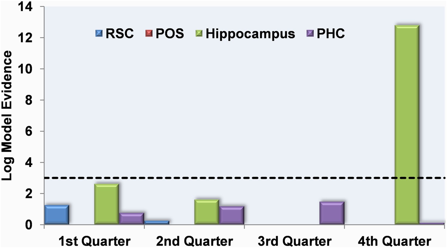
Multivariate Bayes analysis of responses which mapped onto knowledge of permanent landmark locations.
The log model evidence values for response patterns within the RSC (blue), posterior POS (red), hippocampus (HC; green) and parahippocampal cortex (PHC; purple) relating to knowledge of permanent landmark locations are shown in each of the four quarters of scanning. By the final quarter of learning, the pattern of activity in the HC mapped onto the amount subjects knew about where permanent landmarks were located in the environment. The dashed black line indicates the threshold at which log model evidence values are considered to be strong (see ‘Materials and methods’).
Videos
Video 1
This is a short clip from one of the videos which subjects viewed inside the MRI scanner when learning the environment.
It demonstrates the first-person perspective presented to subjects and shows how, when a landmark emerges through the fog, the camera turns to bring it into the centre of view whilst continuing along the path. It also provides an example of what happens at an intersection. See also Figure 2.
Tables
Table 1
Correlations between features of the 60 ‘alien’ landmarks
| Permanence: actual | Permanence: post-scan | Salience: beh'al study | Salience: post-scan | Size: actual | Size: post-scan | |
|---|---|---|---|---|---|---|
| Permanence: actual | 1.000 | – | – | – | – | – |
| – | – | – | – | – | – | |
| Permanence: post-scan | 0.793† | 1.000 | – | – | – | – |
| <0.0001 | – | – | – | – | – | |
| Salience: beh'al study | 0.087 | −0.001 | 1.000 | – | – | – |
| 0.5 | 1.0 | – | – | – | – | |
| Salience: post-scan | 0.315* | 0.325* | 0.314* | 1.000 | – | – |
| 0.01 | 0.01 | 0.02 | – | – | – | |
| Size: actual | 0.000 | 0.068 | 0.088 | 0.428† | 1.000 | – |
| 1.000 | 0.6 | 0.5 | 0.001 | – | – | |
| Size: post-scan | 0.117 | 0.093 | 0.129 | 0.749† | 0.726† | 1.000 |
| 0.4 | 0.5 | 0.3 | <0.0001 | <0.0001 | – |
-
Beh'al = ratings that came from the initial behavioural landmark characterisation study. Correlations are shown between: mean salience scores from the initial characterisation study, the actual size and permanence of landmarks in Fog World, and ratings of permanence, salience and size from the fMRI subjects post-fMRI scan. Each cell shows the Pearson correlation r value above the corresponding p value. Significant correlations are highlighted in bold text.
-
*
Correlation is significant at the 0.05 level (2-tailed).
-
†
Correlation is significant at the 0.01 level (2-tailed).
Download links
A two-part list of links to download the article, or parts of the article, in various formats.
Downloads (link to download the article as PDF)
Open citations (links to open the citations from this article in various online reference manager services)
Cite this article (links to download the citations from this article in formats compatible with various reference manager tools)
A central role for the retrosplenial cortex in de novo environmental learning
eLife 4:e09031.
https://doi.org/10.7554/eLife.09031


