Impact of the scale-up of piped water on urogenital schistosomiasis infection in rural South Africa
- Africa Health Research Institute, South Africa
- University of KwaZulu-Natal, South Africa
- University College London, United Kingdom
- Navrongo Health Research Centre, Ghana Health Service, Ghana
- Harvard T.H. Chan School of Public Health, United States
- University of Heidelberg, Germany
Figures
Figure 1
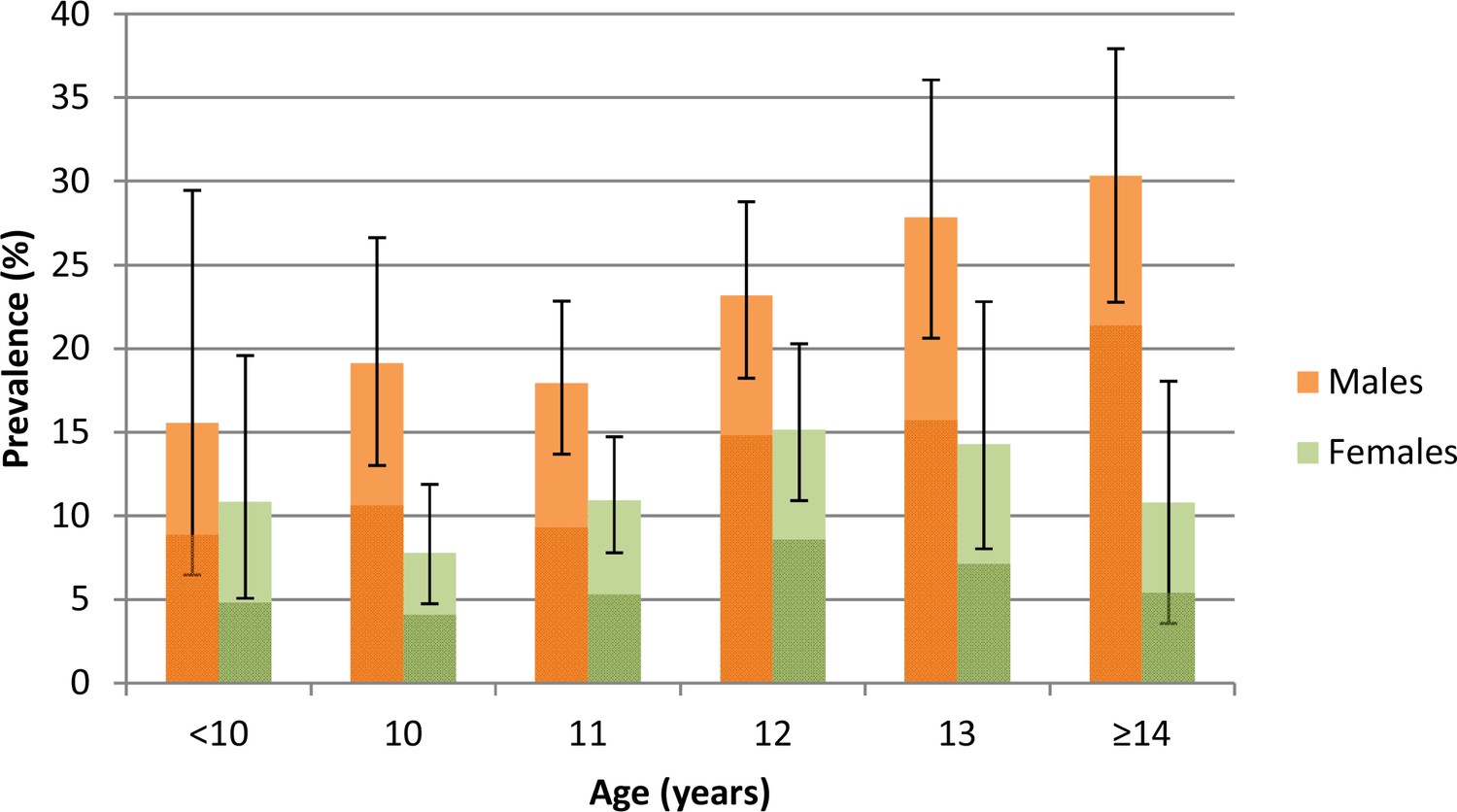
Prevalence (95% CI) of Schistosoma haematobium infection by age and sex among children taking part in the parasitological survey (N = 2,105).
Darker colours represent heavy infections (≥50 eggs per 10 ml urine).
Figure 2
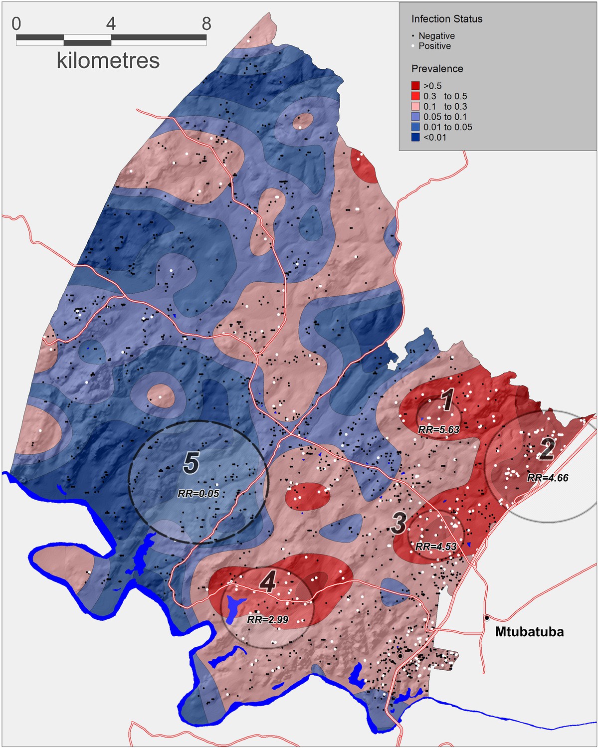
Geographical variations in Schistosoma haematobium prevalence across the surveillance area obtained by a Gaussian kernel applied to participants’ precise household locations.
Approximate locations of participants’ households are shown (incorporating an intentional random error) with white dots representing an infected child. Superimposed on the map are the clusters of infection independently identified by the Kulldorff spatial scan statistic (cluster 5, low relative-risk; cluster 1–4, high relative-risk). The National Road can be seen running along the Eastern boundary of the surveillance area towards Mozambique.
Figure 3
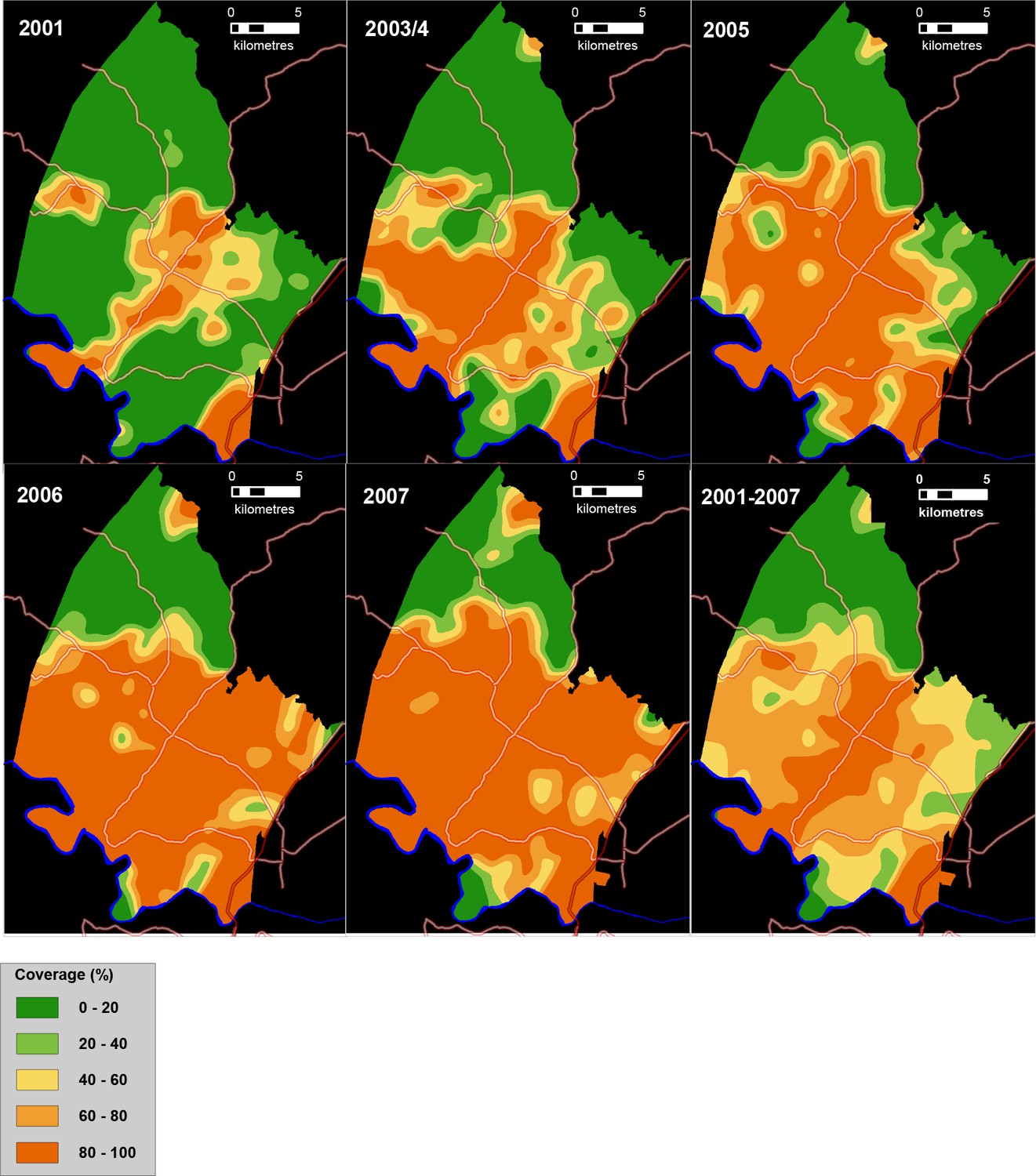
Time series of maps showing the coverage of piped water (%) between 2001 and 2007 in the study area (as measured using a Gaussian kernel approach) as well as mean piped water coverage over the full study period (bottom right).
Main roads are superimposed.
Figure 4 with 1 supplement

Adjusted odds ratio of Schistosoma haematobium infection (95% CI) by piped water coverage in the surrounding local community - coverage quintile (Left) and continuous piped water coverage (Right).
The piped water coverage measure (2001–2007) is derived using a Gaussian kernel to calculate the proportion of all households in the unique local community surrounding each participant having access to piped water (Figure 3). Odds ratios are adjusted for age, sex, household assets, toilet in household, landcover class, distance to water body, altitude, slope, treatment in the last 12 months and school grade. Standard errors are adjusted for clustering by school and grade.
Figure 4—figure supplement 1
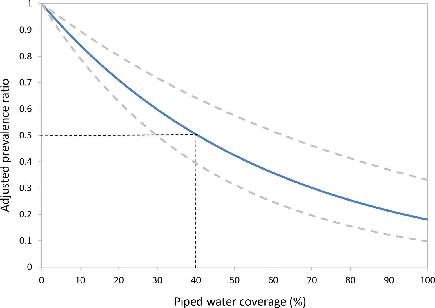
Results of a parallel analysis using a Poisson regression.
The graph shows the adjusted prevalence ratio (95% CI) by piped water coverage in the surrounding local community. The piped water coverage measure (2001–2007) is derived using a Gaussian kernel to calculate the proportion of all households in the unique local community surrounding each participant having access to piped water (Figure 3). The resulting risk estimates are adjusted for age, sex, household assets, toilet in household, landcover class, distance to water body, altitude, slope, treatment in the last 12 months and school grade. Standard errors are adjusted for clustering by school and grade.
Figure 5
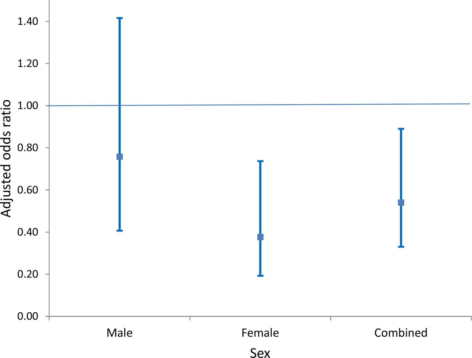
Comparison of adjusted odds of Schistosoma haematobium infection (95% CI) in participants living in households with access to piped water (relative to participants without household-access to piped water) by sex.
The resulting risk estimates are adjusted for age, household assets, toilet in household, landcover class, distance to water body, altitude, slope, treatment in the last 12 months and school grade. Standard errors are adjusted for clustering by school and grade.
Figure 6
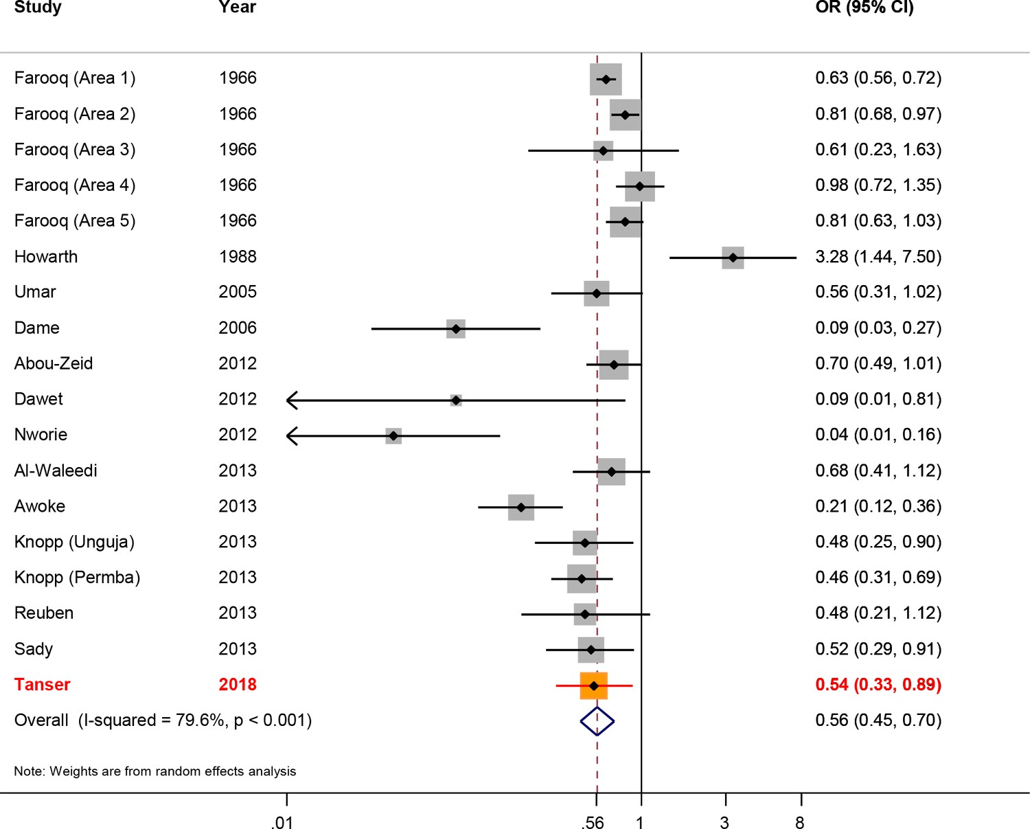
Forest plot of Schistosoma haematobium infection according to household/individual level access to a safe water.
The data are taken from Grimes et al. systematic review (Grimes et al., 2014), based on 17 data-points (Abou-Zeid et al., 2012; Al-Waleedi et al., 2013; Awoke et al., 2013; Dame et al., 2006; Dawet, 2012; Farooq et al., 1966; Howarth et al., 1988; Knopp et al., 2013; Nworie et al., 2012; Reuben et al., 2013; Sady et al., 2013) to which we have added our study results. The sizes of the squares represent the weight given to each study, the rhombus is the effect-size with the black lines representing the 95% confidence intervals. The overall rhombus represents the combined effect-size, with the results of this study shown in red.
Figure 7
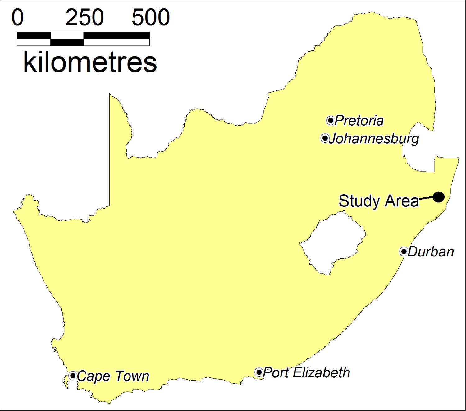
Location of the study area in South Africa.
https://doi.org/10.7554/eLife.33065.013
Figure 8
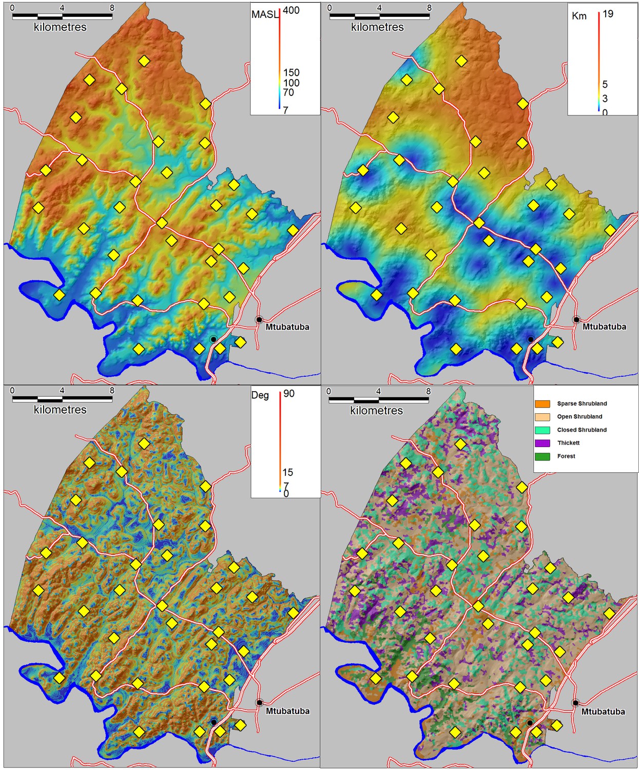
Environmental control variables used in the statistical analysis with locations of 33 schools superimposed (yellow diamonds).
(Top left) Altitude in metres above sea level (MASL) (Top right) Distance to nearest water body (km) (Bottom left) Slope (degrees) (Bottom right) Satellite-derived landcover classification.
Tables
Table 1
Characteristics of the primary school children within the survey who were linked to the population-based cohort (N=1976).
https://doi.org/10.7554/eLife.33065.003| Covariate | Total | Infected (%) | (95% CI) |
|---|---|---|---|
| Gender | |||
| Female | 1016 | 117 (11.5) | (7.7–16.9) |
| Male | 960 | 217 (22.6) | (17.5–28.7) |
| Age group | |||
| 9 | 118 | 14 (11.9) | (7.1–19.2) |
| 10 | 366 | 44 (12.0) | (6.8–20.3) |
| 11 | 592 | 87 (14.7) | (11.3–18.9) |
| 12 | 469 | 92 (19.6) | (13.6–27.4) |
| 13 | 222 | 49 (22.1) | (15.8–30.0) |
| ≥14 | 209 | 48 (23.0) | (15.1–33.3) |
| Community piped water (quintiles)* | |||
| (Lowest) 1 | 399 | 102 (25.6) | (13.0–44.1) |
| 2 | 415 | 87 (21.0) | (15.7–27.4) |
| 3 | 397 | 65 (16.4) | (10.5–24.6) |
| 4 | 386 | 33 (8.5) | (5.4–13.2) |
| 5 | 379 | 47 (12.4) | (8.9–16.9) |
| Household access to water | |||
| No piped water | 304 | 53 (17.4) | (9.9–28.8) |
| Piped water | 1672 | 281 (16.8) | (12.9–21.6) |
| Household assets quintiles | |||
| (Poorest) 1 | 398 | 83 (20.9) | (13.3–31.1) |
| 2 | 387 | 63 (16.3) | (11.7–22.1) |
| 3 | 389 | 63 (16.2) | (11.7–22.0) |
| 4 | 365 | 56 (15.3) | (11.5–20.1) |
| 5 | 359 | 57 (15.9) | (10.4–23.6) |
| Missing | 78 | 12 (15.4) | (9.5–23.9) |
| School grade | |||
| Grade 5 | 1039 | 186 (17.9) | (12.2–25.5) |
| Grade 6 | 937 | 148 (15.8) | (10.4–23.2) |
| Praziquantel in the last 12 months | |||
| No | 1933 | 321 (16.6) | (12.5–21.8) |
| Yes | 43 | 13 (30.2) | (17.3–47.3) |
| Altitude (meters above sea level) | |||
| <50 | 76 | 29 (38.2) | (19.3–61.4) |
| 50–100 | 641 | 168 (26.2) | (19.2–34.7) |
| 100–150 | 875 | 108 (12.3) | (9.5–16.0) |
| 150–200 | 296 | 22 (7.4) | (4.4–12.4) |
| >200 | 88 | 7 (8.0) | (3.5–17.2) |
| Distance to water body | |||
| <1 km | 606 | 112 (18.5) | (14.2–23.7) |
| 1–2 km | 618 | 122 (19.7) | (14.0–27.0) |
| 2–3 km | 376 | 68 (18.1) | (10.8–28.7) |
| >3 km | 376 | 32 (8.5) | (5.4–13.2) |
| Toilet in household | |||
| No Toilet | 438 | 64 (14.6) | (9.9–21.1) |
| Toilet | 1538 | 270 (17.6) | (13.3–22.8) |
| Land cover classification | |||
| Closed Shrubland | 787 | 184 (23.3) | (17.6–30.3) |
| Open Shrubland | 696 | 83 (11.9) | (8.8–15.9) |
| Sparse Shrubland | 437 | 52 (11.9) | (8.7–16.0) |
| Thickett | 56 | 15 (26.8) | (14.8–43.4) |
| Slope (quintiles) | |||
| (Lowest) 1 | 390 | 59 (15.1) | (11.0–20.5) |
| 2 | 386 | 72 (18.7) | (12.9–26.3) |
| 3 | 402 | 70 (17.4) | (11.9–24.8) |
| 4 | 404 | 70 (17.3) | (12.4–23.7) |
| 5 | 394 | 63 (16.0) | (11.6–21.6) |
-
*Computes the proportion of households having access to piped water in the unique community surrounding each participant in the study (Figure 3). The Quintile (Q) ranges (min–max) are: Q1: 0–36; Q2: 37–59; Q3: 60–75; Q4: 76–92; Q5: 93–100.
Table 2
Significant spatial clusters (either unexpectedly high or low numbers) of Schistosoma haematobium infections identified by the Kulldorff spatial scan statistic (p<0.05) across the study area (see Figure 2)
https://doi.org/10.7554/eLife.33065.005| Cluster Number | Radius (km) | Log-Likelihood | P-value | Prevalence (%) | Relative Risk |
|---|---|---|---|---|---|
| 1 | 0.95 | 16.54 | <0.001 | 84.6 | 5.63 |
| 2 | 2.68 | 65.5 | <0.001 | 50 | 4.66 |
| 3 | 1.19 | 30.15 | <0.001 | 49.2 | 4.53 |
| 4 | 1.96 | 14.89 | 0.002 | 41.9 | 2.99 |
| 5 | 2.93 | 17.2 | <0.001 | 0.76 | 0.05 |
Table 3
Logistic regression analysis of the risk factors of Schistosoma haematobium infection.
Model 0 gives the univariate results and Model 1 includes all variables in the model. In Model 2, piped water coverage in the immediate community surrounding each participant has been substituted with household-level piped water covariate.
| Model 0: Univariate | Model 1: Community coverage | Model 2: Household access | |||||||
|---|---|---|---|---|---|---|---|---|---|
| Covariate | aOR | (95% CI) | P-value | aOR | (95% CI) | P-value | aOR | (95% CI) | P-value |
| Community piped water quintiles (vs Lowest)† | |||||||||
| 2 | 0.77 | (0.34, 1.75) | 0.529 | 0.39‡ | (0.23, 0.66) | <0.001 | |||
| 3 | 0.57 | (0.22, 1.50) | 0.250 | 0.30 | (0.15, 0.59) | <0.001 | |||
| 4 | 0.27 | (0.10, 0.71) | 0.009 | 0.16 | (0.08, 0.33) | <0.001 | |||
| 5 | 0.41 | (0.17, 0.99) | 0.048 | 0.12 | (0.06, 0.26) | <0.001 | |||
| Household access to water (vs No) | |||||||||
| Yes | 0.96 | (0.56, 1.64) | 0.870 | 0.54 | (0.33, 0.89) | 0.017 | |||
| Gender (vs Female) | |||||||||
| Male | 2.24 | (1.64, 3.08) | <0.001 | 2.62 | (1.92, 3.59) | <0.001 | 2.41 | (1.77, 3.28) | <0.001 |
| Age testing | |||||||||
| Per unit | 1.19 | (1.07, 1.31) | 0.001 | 1.21 | (1.08, 1.36) | 0.001 | 1.18 | (1.06, 1.31) | 0.002 |
| Grade (vs Grade 5) | |||||||||
| Grade 6 | 0.86 | (0.45, 1.66) | 0.648 | 0.76 | (0.51, 1.11) | 0.149 | 0.77 | (0.47, 1.28) | 0.310 |
| Praziquantel in last 12 months (vs No) | |||||||||
| Yes | 2.18 | (1.05, 4.52) | 0.038 | 1.27 | (0.60, 2.71) | 0.529 | 1.48 | (0.69, 3.16) | 0.307 |
| Altitude Class (vs < 50) | |||||||||
| 50–100 | 0.58 | (0.27, 1.22) | 0.147 | 0.47 | (0.23, 0.96) | 0.039 | 0.50 | (0.23, 1.09) | 0.081 |
| 100–150 | 0.23 | (0.09, 0.60) | 0.003 | 0.20 | (0.09, 0.43) | <0.001 | 0.20 | (0.08, 0.51) | 0.001 |
| 150–200 | 0.13 | (0.04, 0.39) | <0.001 | 0.09 | (0.03, 0.25) | <0.001 | 0.11 | (0.04, 0.33) | <0.001 |
| >200 | 0.14 | (0.04, 0.51) | 0.004 | 0.08 | (0.03, 0.29) | <0.001 | 0.12 | (0.03, 0.44) | 0.002 |
| Landcover class (vs Sparse Shrubland) | |||||||||
| Closed Shrubland | 2.26 | (1.55, 3.28) | <0.001 | 1.56 | (1.05, 2.31) | 0.030 | 2.41 | (1.63, 3.58) | <0.001 |
| Open Shrubland | 1.00 | (0.70, 1.44) | 0.989 | 1.03 | (0.72, 1.47) | 0.863 | 1.44 | (0.96, 2.17) | 0.079 |
| Thickett | 2.71 | (1.28, 5.75) | 0.010 | 1.75 | (0.82, 3.73) | 0.145 | 2.52 | (1.23, 5.18) | 0.012 |
| Slope (square root) | |||||||||
| per unit | 0.98 | (0.83, 1.16) | 0.818 | 1.02 | (0.89, 1.16) | 0.794 | 0.91 | (0.79, 1.04) | 0.159 |
| Distance to water body (vs < 1 km) | |||||||||
| 1–2 km | 1.08 | (0.74, 1.58) | 0.667 | 0.78 | (0.56, 1.08) | 0.131 | 0.99 | (0.69, 1.41) | 0.946 |
| 2–3 km | 0.97 | (0.54, 1.75) | 0.928 | 0.72 | (0.47, 1.12) | 0.143 | 1.04 | (0.62, 1.77) | 0.874 |
| >3 km | 0.41 | (0.23, 0.74) | 0.003 | 0.25 | (0.12, 0.49) | <0.001 | 0.44 | (0.24, 0.79) | 0.007 |
| Toilet in household (vs No) | |||||||||
| Yes | 1.24 | (0.90, 1.72) | 0.186 | 1.24 | (0.87, 1.76) | 0.229 | 1.20 | (0.84, 1.72) | 0.319 |
| Household assets quintile (vs Poorest) | |||||||||
| 2 | 0.74 | (0.50, 1.09) | 0.123 | 0.88 | (0.60, 1.27) | 0.480 | 0.87 | (0.61, 1.25) | 0.459 |
| 3 | 0.73 | (0.49, 1.09) | 0.127 | 0.78 | (0.51, 1.18) | 0.235 | 0.75 | (0.48, 1.16) | 0.186 |
| 4 | 0.69 | (0.42, 1.14) | 0.143 | 0.81 | (0.47, 1.40) | 0.450 | 0.67 | (0.40, 1.11) | 0.118 |
| 5 | 0.72 | (0.41, 1.24) | 0.228 | 0.80 | (0.48, 1.34) | 0.389 | 0.62 | (0.36, 1.05) | 0.075 |
| Missing | 0.69 | (0.39, 1.21) | 0.194 | 0.84 | (0.40, 1.80) | 0.658 | 0.64 | (0.29, 1.40) | 0.258 |
-
† Computes the proportion of households having access to piped-water in the unique community surrounding each participant in the study (Figure 3). The Quintile (Q) ranges (min–max) are: Q1: 0–36; Q2: 37–59; Q3: 60–75; Q4: 76–92; Q5: 93–100, ‡ Corresponding values for a model in which community-level piped-water coverage is used as a continuous variable: a 1% increase in the coverage of piped-water in the surrounding community, was independently associated with a 2.5% decrease in the odds of a Schistosoma haematobium infection (aHR=0.975; 95% CI: 0.966, 0.985; p-value<0.001).
Table 4
Multivariable model examining the socio-demographic predictors of Schistosoma haematobium infection stratified by gender.
Model 1 includes all variables in the model. In Model 2, piped water coverage in the immediate community surrounding each participant has been substituted with household-level piped water covariate.
| Model 1: Community-level coverage of piped water | Model 2: Household level access to piped water | ||||||||
|---|---|---|---|---|---|---|---|---|---|
| Females | Males | Females | Males | ||||||
| Covariate | aOR§ (95% CI) | P-value | aOR§ (95% CI) | P-value | aOR§ (95% CI) | P-value | aOR§ (95% CI) | P-value | |
| Community piped water quintiles (vs Lowest)† | |||||||||
| 2 | 0.24 (0.10–0.57)‡ | 0.002 | 0.56 (0.35–0.90)‡ | 0.017 | |||||
| 3 | 0.21 (0.08–0.55) | 0.002 | 0.37 (0.17–0.78) | 0.011 | |||||
| 4 | 0.16 (0.06–0.45) | 0.001 | 0.16 (0.08–0.35) | <0.001 | |||||
| 5 | 0.07 (0.02–0.20) | <0.001 | 0.17 (0.08–0.36) | <0.001 | |||||
| Household access to water (vs No) | |||||||||
| Yes | 0.38 (0.19–0.75) | 0.005 | 0.76 (0.41–1.42) | 0.379 | |||||
| Age at Testing | |||||||||
| Per unit | 9.62 (1.62–57.22) | 0.014 | 1.24 (1.08–1.42) | 0.003 | 6.85 (1.56–30.16) | 0.011 | 1.20 (1.06–1.37) | 0.005 | |
| Age2 | |||||||||
| Per unit | 0.92 (0.85–0.99) | 0.024 | 0.93 (0.88–0.99) | 0.017 | |||||
| Toilet in household (vs No) | |||||||||
| Yes | 1.59 (0.88–2.88) | 0.121 | 1.12 (0.70–1.86) | 0.667 | 1.26 (0.75–2.14) | 0.371 | 1.11 (0.66–1.86) | 0.687 | |
| Household Assets quintile (vs Poorest) | |||||||||
| 2 | 0.46 (0.24–0.90) | 0.026 | 1.27 (0.75–2.08) | 0.344 | 0.55 (0.30–0.99) | 0.045 | 1.24 (0.76–2.04) | 0.376 | |
| 3 | 0.35 (0.13–0.89) | 0.032 | 1.21 (0.72–1.99) | 0.453 | 0.35 (0.15–0.84) | 0.019 | 1.19 (0.71–1.98) | 0.502 | |
| 4 | 0.42 (0.18–1.00) | 0.061 | 1.18 (0.55–2.28) | 0.646 | 0.40 (0.18–0.91) | 0.029 | 0.94 (0.46–1.94) | 0.885 | |
| 5 | 0.66 (0.32–1.37) | 0.307 | 0.90 (0.43–1.75) | 0.769 | 0.54 (0.25–1.17) | 0.115 | 0.71 (0.34–1.44) | 0.337 | |
| Missing | 0.57 (0.20–1.66) | 0.288 | 1.10 (0.38–2.94) | 0.815 | 0.40 (0.12–1.35) | 0.135 | 0.91 (0.34–2.42) | 0.845 | |
-
§All estimates simultaneously adjusted for landcover class, distance to water, altitude, slope, treatment in the last 12 months and school grade.
† Computes the proportion of households having access to piped-water in the unique community surrounding each participant in the study (Figure 3). The Quintile (Q) ranges (min–max) are: Q1: 0–36; Q2: 37–59; Q3: 60–75; Q4: 76–92; Q5: 93–100
Additional files
-
Supplementary file 1
Shows the adjusted prevalence ratios (aPR) for the risk factors of Schistosoma haematobium infection, which are parallel to the results presented in Table 3.
Model 0 gives the univariate results and Model 1 includes all variables in the model. In Model 2, piped water coverage in the immediate community surrounding each participant has been substituted with the household-level piped water covariate.
- https://doi.org/10.7554/eLife.33065.015
-
Supplementary file 2
Linear probability regression models showing the impact of piped water on schistosomiasis infection in primary school children across the study area.
Model 0 gives the univariate results and Model 1 gives the multivariate results for the availability of piped water in the community. Model 2 shows the instrumental variable estimation (IVE) results corresponding to Model 1, where the instrumental variable is the year that piped water was introduced into the community. Model 3 gives the multivariate results for piped water in the household and Model 4 shows the corresponding IVE results.
- https://doi.org/10.7554/eLife.33065.016
-
Transparent reporting form
- https://doi.org/10.7554/eLife.33065.017
Download links
A two-part list of links to download the article, or parts of the article, in various formats.
Downloads (link to download the article as PDF)
Open citations (links to open the citations from this article in various online reference manager services)
Cite this article (links to download the citations from this article in formats compatible with various reference manager tools)
Impact of the scale-up of piped water on urogenital schistosomiasis infection in rural South Africa
eLife 7:e33065.
https://doi.org/10.7554/eLife.33065


