One-shot learning and behavioral eligibility traces in sequential decision making
- École Polytechnique Fédérale de Lausanne, Switzerland
- Swiss Center for Affective Sciences, University of Geneva, Switzerland
Figures
Figure 1
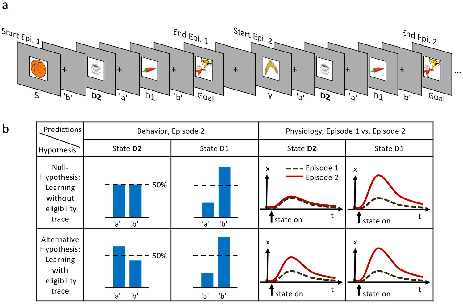
Experimental design and hypothesis.
(a) Typical state-action sequences of the first two episodes. At each state, participants execute one of two actions, ’a’ or ’b’, leading to the next state. Here, the participant discovered the goal state after randomly choosing three actions: ’b’ in state S (Start), ’a’ in D2 (two actions from the goal), and ’b’ in D1 (one action from the goal). Episode 1 terminated at the rewarding goal state. Episode 2 started in a new state, Y. Note that D2 and D1 already occurred in episode 1. In this example, the participant repeated the actions which led to the goal in episode 1 (’a’ at D2 and ’b’ at D1). (b) Reinforcement learning models make predictions about such behavioral biases, and about learned properties (such as action value , state value or TD-errors, denoted as ) presumably observable as changes in a physiological measure (e.g. pupil dilation). Null Hypothesis: In RL without eligibility traces, only the state-action pair immediately preceding a reward is reinforced, leading to a bias at state D1, but not at D2 (50%-line). Similarly, the state value of D2 does not change and therefore the physiological response at the D2 in episode 2 (solid red line) should not differ from episode 1 (dashed black line). Alternative Hypothesis: RL with eligibility traces reinforces decisions further back in the state-action history. These models predict a behavioral bias at D1 and D2, and a learning-related physiological response at the onset of these states after a single reward. The effects may be smaller at state D2 because of decay factors in models with eligibility traces.
Figure 2
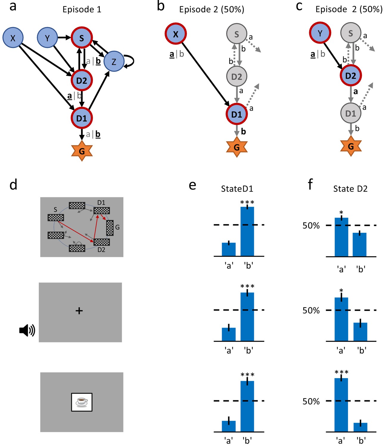
A single delayed reward reinforces state-action associations.
(a) Structure of the environment: six states, two actions, rewarded goal G. Transitions (arrows) were predefined, but actions were attributed to transitions during the experiment. Unbeknownst to the participants, the first actions always led through the sequence S (Start), D2 (two steps before goal), D1 (one step before goal) to G (Goal). Here, the participant chose actions ’b’, ’a’, ’b’ (underlined boldface). (b) Half of the experiments, started episode 2 in X, always leading to D1, where we tested if the action rewarded in episode 1 was repeated. (c) In the other half of experiments, we tested the decision bias in episode 2 at D2 (’a’ in this example) by starting from Y. (d) The same structure was implemented in three conditions. In the spatial condition (22 participants, top row in Figures (d), (e) and (f)), each state is identified by a fixed location (randomized across participants) of a checkerboard, flashed for a 100 ms on the screen. Participants only see one checkerboard at a time; the red arrows and state identifiers S, D2, D1, G are added to the figure to illustrate a first episode. In the sound condition (15 participants, middle row), states are represented by unique short sounds. In the clip-art condition (12 participants, bottom row), a unique image is used for each state. (e) Action selection bias in state D1, in episode 2, averaged across all participants. (f) In all three conditions the action choices at D2 were significantly different from chance level (dashed horizontal line) and biased toward the actions that have led to reward in episode 1. Error bars: SEM, , . For clarity, actions are labeled ’a’ and ’b’ in (e) and (f), consistent with panels (a) - (c), even though actual choices of participants varied.
Figure 3
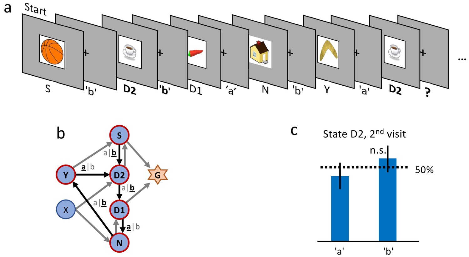
Control experiment without reward.
(a) Sequence of the first six state-action pairs in the first control experiment. The state D2 is visited twice and the number of states between the two visits is the same as in the main experiment. The original goal state has been replaced by a non-rewarded state N. The control experiment focuses on the behavior during the second visit of state D2, further state-action pairs are not relevant for this analysis. (b) The structure of the environment has been kept as close as possible to the main experiment (Figure 2 (a)). (c) Ten participants performed a total of 32 repetitions of this control experiment. Participants show an average action-repetition bias of 56%. This bias is not significantly different from the 50% chance level () and much weaker than the 85% observed in the main experiment (Figure 2 (f)).
Figure 4
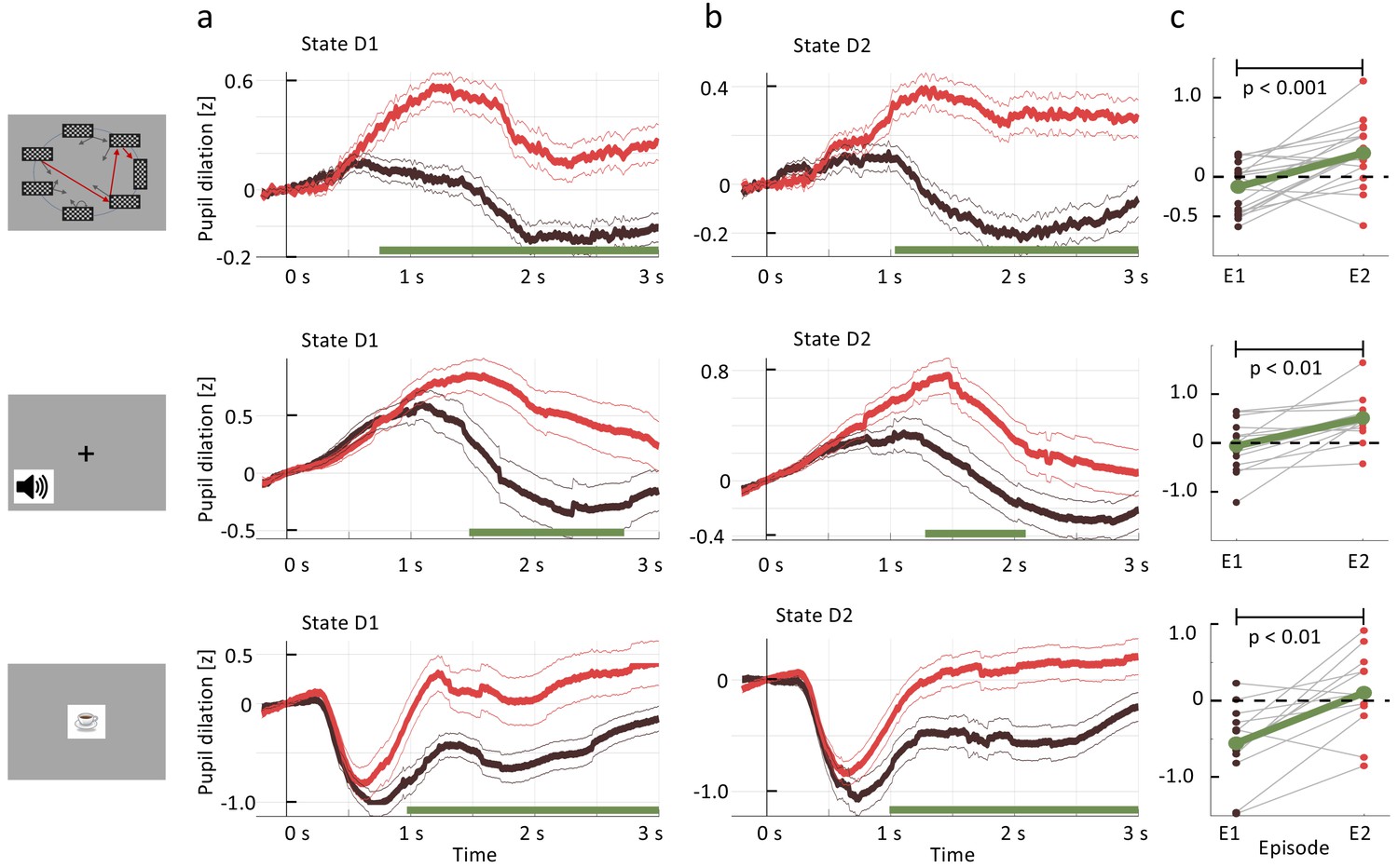
Pupil dilation reflects one-shot learning.
(a) Pupil responses to state D1 are larger during episode 2 (red curve) than during episode 1 (black). (b) Pupil responses to state D2 are larger during episode 2 (red curve) than during episode 1 (black). Top row: spatial, middle row: sound, bottom row: clip-art condition. Pupil diameter averaged across all participants in units of standard deviation (z-score, see Materials and methods), aligned at stimulus onset and plotted as a function of time since stimulus onset. Thin lines indicate the pupil signal ± SEM. Green lines indicate the time interval during which the two curves differ significantly (). Significance was reached at a time , which depends on the condition and the state: spatial D1: (22, 131, 85); spatial D2: (22, 137,130) sound D1: (15, 34, 19); sound D2: (15, 35, 33); clip-art D1: (12, 39, 19); clip-art D2: (12, 45, 41); (Numbers in brackets: number of participants, number of pupil traces in episode 1 or 2, respectively). (c) Participant-specific mean pupil dilation at state D2 (averaged over the interval (1000 ms, 2500 ms)) before (black dot) and after (red dot) the first reward. Grey lines connect values of the same participant. Differences between episodes are significant (paired t-test, p-values indicated in the Figure).
Figure 5
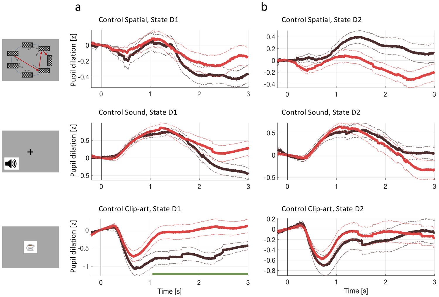
Pupil dilation during the second control experiment.
In the second control experiment, different participants passively observed state sequences which were recorded during the main experiment. Data analysis was the same as for the main experiment. (a) Pupil time course after state onset () of state D1 (before goal). (b) State D2 (two before goal). Black traces show the pupil dilation during episode one, red traces during episode two. At state D1 in the clip-art condition, the pupil time course shows a separation similar to the one observed in the main experiment. This suggest that participants may recognize the clip-art image that appears just before the final image. Importantly in state D2, the pupil time course during episode 2 is qualitatively different from the one in the main experiment (Figure 4).
Figure 6

Reward prediction error (RPE) at non-goal states modulates pupil dilation.
Pupil traces (in units of standard deviation) from all states except G were aligned at state onset () and the mean pupil response was subtracted (see Materials and methods). (a) The deviation from the mean is shown for states where the model predicts (black, dashed) and for states where the model predicts percentile (solid, blue). Shaded areas: ± SEM. Thus the pupil dilation reflects the RPE predicted by a reinforcement learning model that spreads value information to nonrewarded states via eligibility traces. (b) To qualitatively distinguish pupil correlations with RPE from correlations with state values , we started from the following observation: the model predicts that RPE decreases over the course of learning (due to convergence), while the state values increase (due to spread of value information). We wanted to observe this qualitative difference in the pupil dilations of subsequent visits of the same state. We selected pairs of visits and for which the RPE decreased while increased and extracted the pupil measurements of the two visits (again, mean is subtracted). The dashed, black curves show the average pupil trace during the visit of a state. The solid black curves correspond to the next visit () of the same state. In the spatial condition, the two curves significantly () separate at (indicated by the green line). All three conditions show the same trend (with strong significance in the spatial condition), compatible with a positive correlation of pupil response with RPE, but not with state value . (c) The mean pupil dilation is different in each condition, whereas the learning related deviations from the mean (in (a) and (b)) have similar shapes.
Figure 7
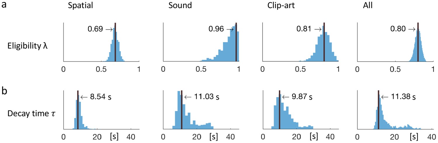
Eligibility for reinforcement decays with a time-scale in the order of 10 s.
The behavioral data of each experimental condition constrain the free parameters of the model Q-λ to the ranges indicated by the blue histograms (see methods) (a) Distribution over the eligibility trace parameter λ in Equation 1 (discrete time steps). Vertical black lines indicate the values that best explain the data (maximum likelihood, see Materials and methods). All values are significantly different from zero. (b) Modeling eligibility in continuous time with a time-dependent decay (Materials and methods, Equation 5), instead of a discrete per-step decay. The behavioral data constrains the time-scale parameter to around 10 s. Values in the column All are obtained by fitting λ and to the aggregated data of all conditions.
Figure 8
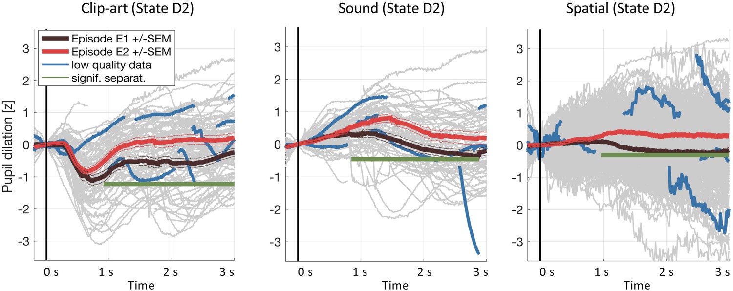
Results including low-quality pupil traces.
We repeated the pupil data analysis at the crucial state D2including all data (including traces with less than 50% of data within the 3s window and with z-values outside ±3). Gray curves in the background show all recorded pupil traces. The highlighted blue curves show a few, randomly selected, low-quality pupil traces. Including these traces does not affect the result.
Figure 9
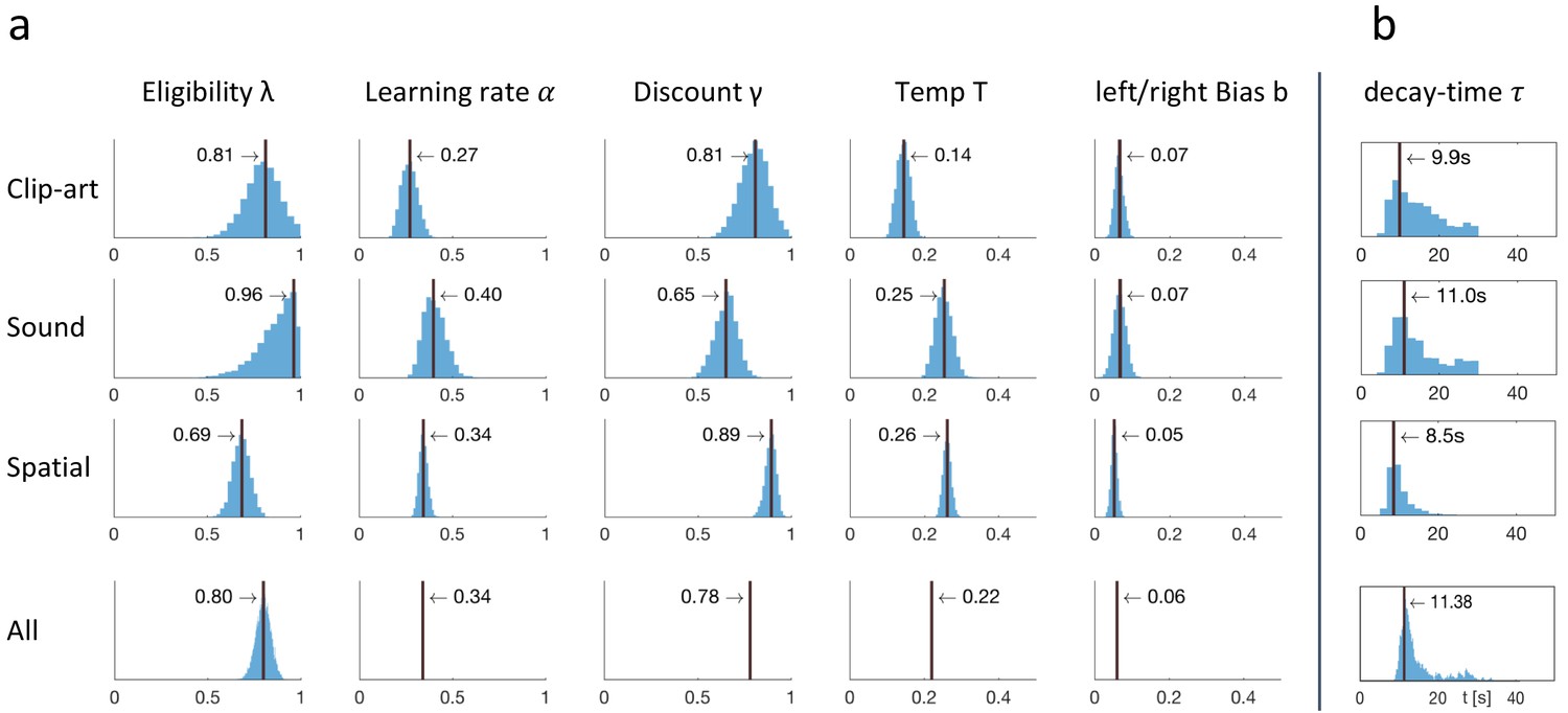
Fitting results: behavioral data constrained the free parameters of Q-λ.
(a) For each experimental condition a distribution over the five free parameters is estimated by sampling. The blue histograms show the approximate conditional posterior for each parameter (see Materials and methods). Vertical black lines indicate the values of the five-parameter sample that best explains the data (maximum likelihood, ML). The bottom row (All) shows the distribution over λ when fitted to the aggregated data of all conditions, with other parameters fixed to the indicated value (mean over the three conditions). (b) Estimation of a time dependent decay ( instead of λ) as defined in Equation 5.
Figure 10

Simulated experiment.
( Q-λ model). (a) and (b): Task structure (same as in Figure 2). Simulated agents performed episodes 1 and 2 and we recorded the decisions at states D1 and D2 in episode 2. (c): Additionally, we also simulated the model’s behavior at state S, by extending the structure of the (simulated) experiment with a new state R, leading to S. (d): We calculated the action-selection bias at states D1, D2 and S during episode 2 from the behavior of (blue) and (green) simulated agents. The effect size (observed during episode 2 and visualized in panel (d)) decreases when (in episode 1) the delay between taking the action and receiving the reward increases. It is thereby smallest at state S. When setting the model’s eligibility trace parameter to 0(red, no ET), the effect at state D1 is not affected (see Equation 1) while at D2 and S the behavior was not reinforced. Horizontal dashed line: chance level 50%. Errorbars: standard deviation of the simulated effect when estimating 1000 times the mean bias from and simulated agents with individually sampled model parameters.
Figure 11
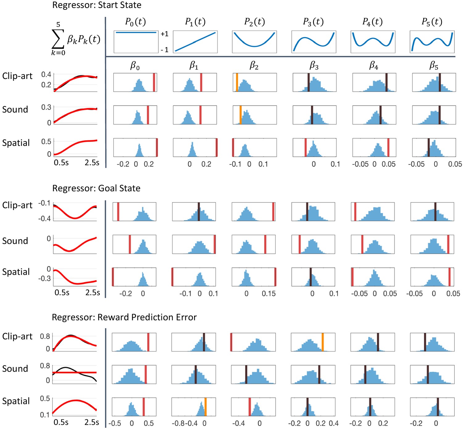
Detailed results of regression analysis and permutation tests.
The regressors are top: Start state event, middle: Goal state event and bottom: Reward Prediction Error. We extracted the time course of the pupil dilation in (500 ms, 2500 ms) after state onset for each of the conditions, clip-art, sound and spatial, using Legendre polynomials of orders k = 0 to k = 5 (top row) as basis functions. The extracted weights (cf. Equation 8) are shown in each column below the corresponding Legendre polynomial as vertical bars with color indicating the level of significance (red, statistically significant at p<0.05/6 (Bonferroni); orange, p<0.05; black, not significant). Blue histograms summarize shuffled samples obtained by 1000 permutations. Black curves in the leftmost column show the fits with all six Legendre Polynomials, while the red curve is obtained by summing only over the few Legendre Polynomials with significant . Note the similarity of the pupil responses across conditions.
Tables
Table 1
Models with eligibility trace explain behavior significantly better than alternative models.
Four reinforcement learning models with eligibility trace (Q-λ, REINFORCE, SARSA-λ, 3-step-Q); two model-based algorithms (Hybrid, Forward Learner), two RL models without eligibility trace (Q-0, SARSA-0), and a null-model (Biased Random, Materials and methods) were fitted to the human behavior, separately for each experimental condition (spatial, sound, clip-art). Models with eligibility trace ranked higher than those without (lower Akaike Information Criterion, AIC, evaluated on all participants performing the condition). indicates the normalized Akaike weights (Burnham and Anderson, 2004), values < 0.01 are not added to the table. Note that only models with eligibility trace have . The ranking is stable as indicated by the sum of rankings (column rank sum) on test data, in -fold crossvalidation (Materials and methods). P-values refer to the following comparisons: P(a): Each model in the with eligibility trace group was compared with the best model without eligibility trace (Hybrid in all conditions); models for which the comparison is significant are shown in bold. P(b): Q-0 compared with Q-λ. P(c): SARSA-0 compared with SARSA-λ. P(d): Biased Random compared with the second last model, which is Forward Learner in the clip-art condition and SARSA-0 in the two others. In the Aggregated column, we compared the same pairs of models, taking into account all ranks across the three conditions. All algorithms with eligibility trace explain the human behavior better (p(e)<.001) than algorithms without eligibility trace. Differences among the four models with eligibility trace are not significant. In each comparison, pairs of individual ranks are used to compare pairs of models and obtain the indicated p-values (Wilcoxon rank-sum test, Materials and methods).
| Condition | Spatial | Sound | Clip-art | Aggregated | ||||
|---|---|---|---|---|---|---|---|---|
| Model | AIC | Rank Sum (k = 11) | AIC | Rank Sum (k = 7) | AIC | Rank Sum (k = 7) | all ranks | |
| With elig tr. | Q-λ | |||||||
| Reinforce | ||||||||
| 3-step-Q | ||||||||
| SARSA-λ | ||||||||
| Model based | Hybrid | |||||||
| Forward Learner | ||||||||
| Without elig tr. | Q-0 | |||||||
| SARSA-0 | ||||||||
| Biased Random | ||||||||
Additional files
Download links
A two-part list of links to download the article, or parts of the article, in various formats.
Downloads (link to download the article as PDF)
Open citations (links to open the citations from this article in various online reference manager services)
Cite this article (links to download the citations from this article in formats compatible with various reference manager tools)
One-shot learning and behavioral eligibility traces in sequential decision making
eLife 8:e47463.
https://doi.org/10.7554/eLife.47463


