Representation of visual landmarks in retrosplenial cortex
- Massachusetts Institute of Technology, United States
Figures
Figure 1 with 1 supplement
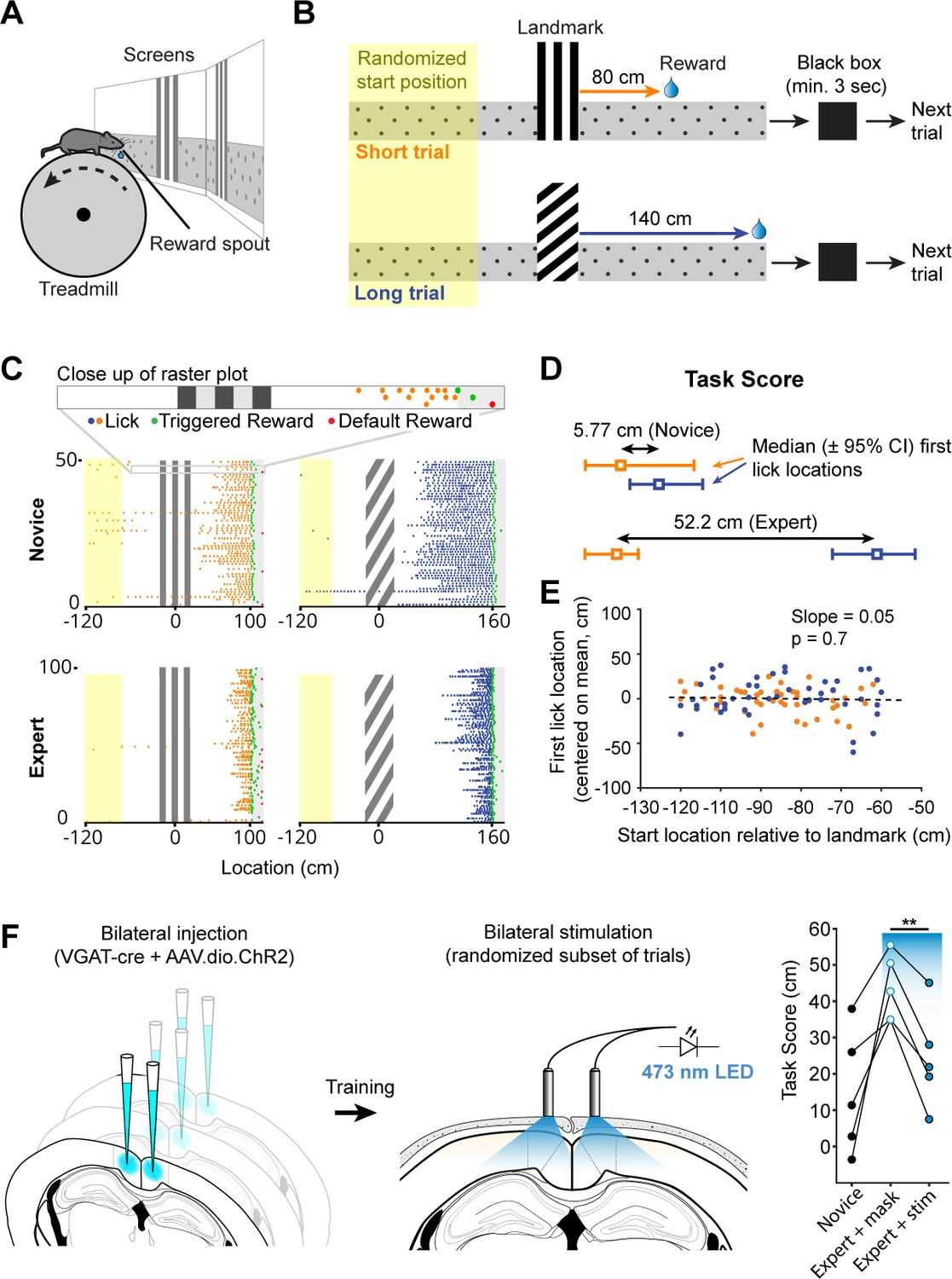
Landmark-dependent navigation task in virtual reality.
(A) Schematic of experimental setup: mice are head-fixed atop a cylindrical treadmill with two computer screens covering most of the animal’s field of view. A reward spout with attached lick-sensor delivers rewards. (B) Task design. Animals learned to locate hidden reward zones at a fixed distance from one of two salient visual cues acting as landmarks. The two landmarks were interleaved within a session, either randomly or in blocks of 5. After each trial animals were placed in a ‘black box’ (screens turn black) for at least 3 s. The randomized starting location ranged from 50 to 150 cm before the landmark. (C) Licking behavior of the same animal at novice and expert stage. Expert animals (bottom) lick close to the reward zones once they have learned the spatial relationship between the visual cue and reward location. (D) The Task Score was calculated as the difference in first lick location (averaged across trials) between short and long trials. (E) Relationship between trial start and first lick locations for one example session. Experimental design ensured that alternative strategies, such as using an internal odometer, could not be used to accurately find rewards. (F) RSC inactivation experiment. VGAT-Cre mice were injected with flexed Channelrhodopsin-2 (left). Stimulation light was delivered through skull-mounted ferrules on a random subset of trials (middle). During inactivation trials, task score was reduced significantly (right).
Figure 1—figure supplement 1
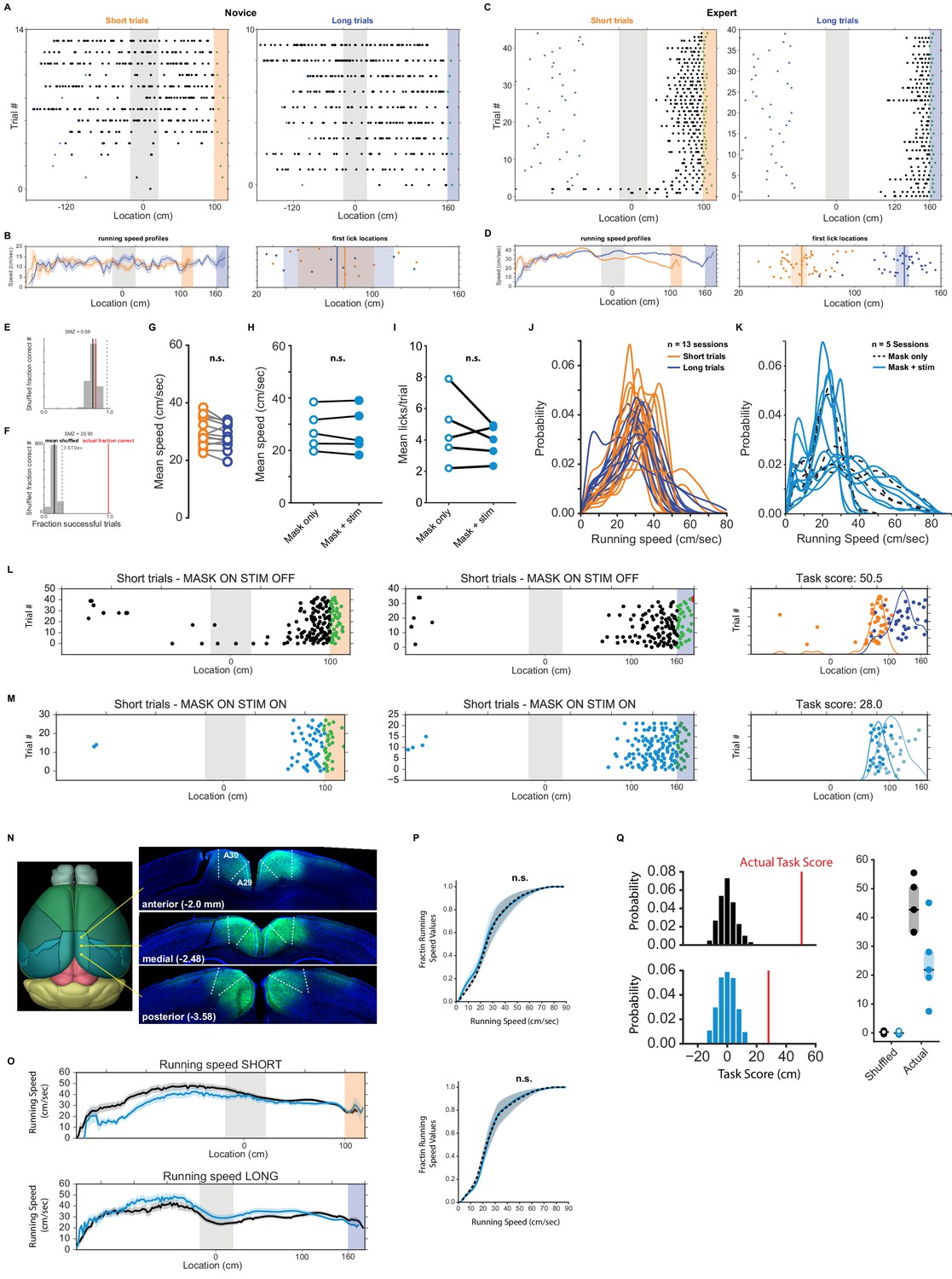
Running and licking behavior in naive animals and during optogenetic silencing.
(A) Raster plot of licking behavior of example session of a novice animal with short and long trials separated. Note: during the recording the trials were interleaved. The blue triangles indicate the start location of each trial. (B) Left: Mean running speed as a function of space (5 cm bins, shaded is standard error of the mean). Right: Location of first licks on short and long trials superimposed. Shaded areas indicate 95% confidence interval. (C, D) Same as A and B but for an expert animal. (E) Spatial modulation z-score (SMZ) for novice animal (shown in (A)). The gray bars represent a histogram of fraction of successful trials when the location of licks was rotated randomly (repeated 1000 times). Dashed line: three standard deviations of that distribution. The red line indicated the animal’s actual fraction of successful trials within that session. (F) SMZ of an expert animal (shown in (B)). (G) Mean running speed on short and long trials for all recording sessions (Wilcoxon signed-rank test: p>0.05) (H) Same analysis as (D) but for running speed during mask only and mask + stimulation trials during optogenetic inactivation sessions. (I) Mean number of licks in mask only vs mask + stim conditions. Overall number of licks was not influenced by stimulation light. (J) Kernel density estimates of running speeds for all recording sessions for short and long trials. (K) Same analysis as (J) but during mask only and mask + stim conditions. (L) Licking behavior in a session where on 50% of trials only the masking light was shown, and the other 50% the masking and optogenetic stimulation light was shown. On short trials (left column) and long trials (center column) when only the masking light was shown. Right column: the first lick per trial on short (orange) and long (blue) trials plotted. (M) Same as (L), but when mask and optogenetic stimulation light was on. (N) ChR2 expression in RSC. A mouse was injected using the same protocol as during the inactivation experiment. (O) Running speed profiles during stimulation and mask-only trials showing small but overall not significant differences between those two conditions. (P) Normalized cumulative distribution of speed values (K-S test: pshort_trials = 1.0, plong_trials = 1.0). (Q) Label-shuffle test of mask-only and stimulation trials. To test whether mice confuse, mis-assign or can’t see/identify landmarks and their respective reward locations we randomly re-assigned the labels of each trial type (short vs. long) and re-calculated the task score. This process was repeated 1000 times and the resulting mean task score compared to the recorded one. We found a significant difference between the shuffled and actual task scores (One-way ANOVA p<0.0001, tukey post-hoc test) suggesting that animals are worse at locating the reward zone based.
Figure 2 with 2 supplements
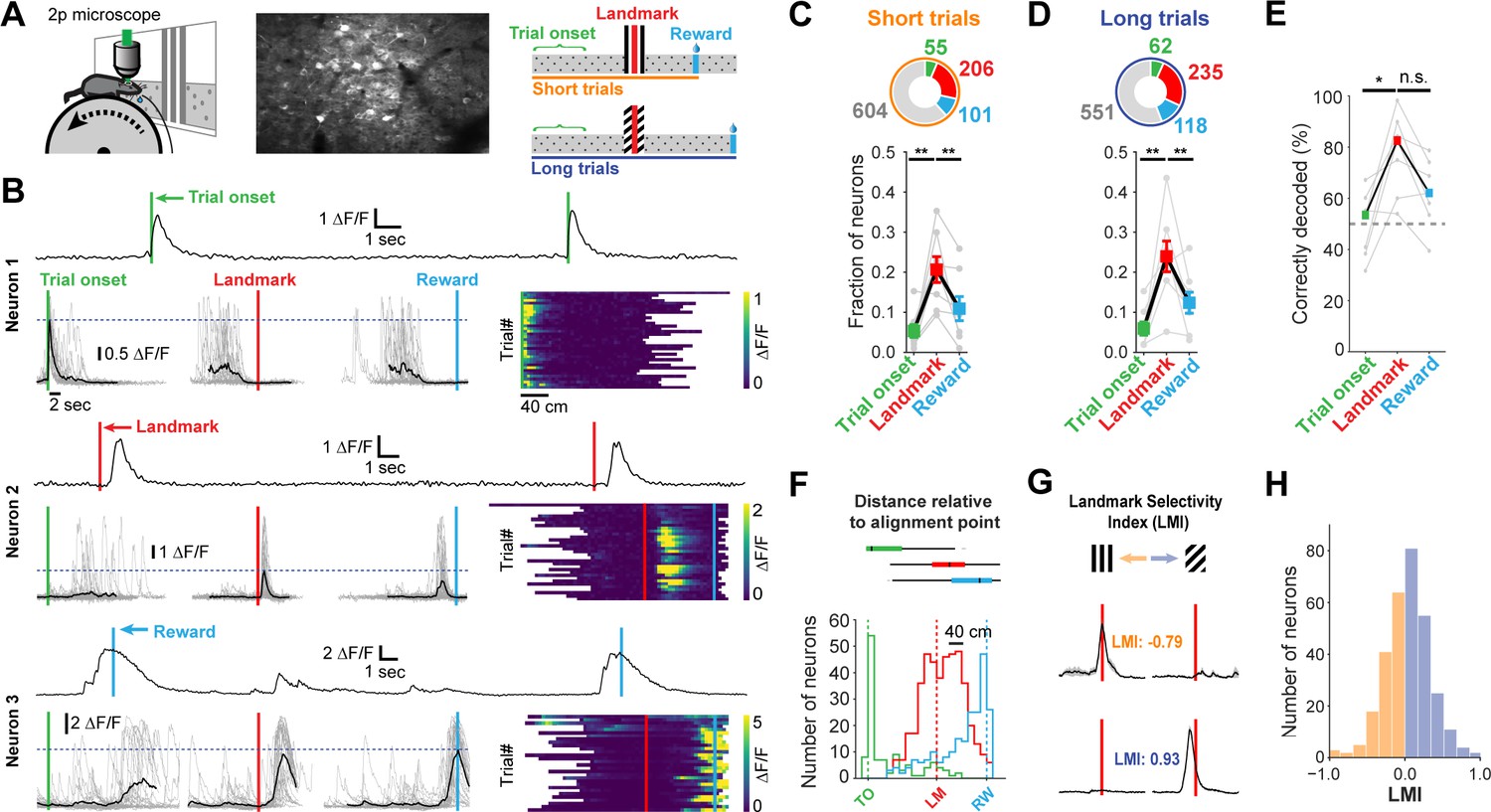
Neuronal responses in RSC during landmark-dependent navigation.
(A) Left: schematic of recording setup. Middle: example field of view. Right: Alignment points and trial types. The activity of each neuron was then aligned to each of three points: trial onset (green), landmark (red), and reward (cyan). Responses were independently analysed for short and long trials. (B) Each neuron’s best alignment point was assessed by quantifying the peak of its mean trace and comparing it to the other alignment points. Rows show trial onset (top), landmark (middle), and reward aligned (bottom) example neurons. (C, D) Alignment of task-active neurons. The majority of task-engaged neurons were aligned to the landmark on short (C) and long (D) trials (n = 7 mice). (E) We applied a template matching decoder (Montijn et al., 2014) to decode the trial type based on the neural responses recorded from each animal. Trial onset neurons provided chance level decoding. However, landmark neurons provided significantly higher decoding accuracy which remained elevated for reward neurons (F) Mean distance of transient peaks of individual neurons relative to alignment point. (G) Two landmark-selective neurons. Landmark selectivity was calculated as the normalized difference between peak mean responses. (H) The landmark selectivity index (LMI) of all landmark neurons shows a unimodal distribution.
Figure 2—figure supplement 1
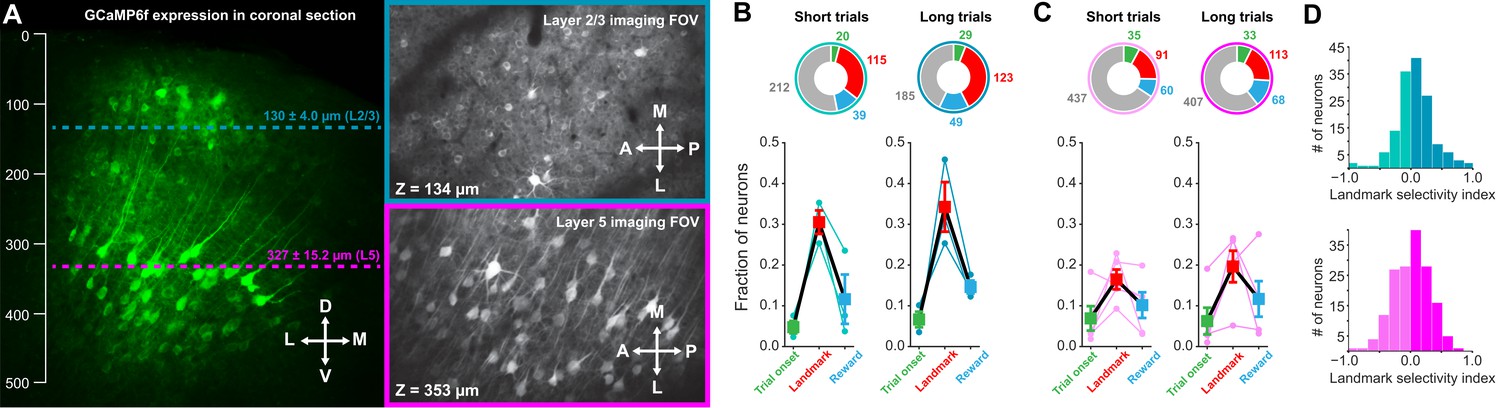
Differences in landmark encoding in layer 2/3 and layer 5.
RSC does not contain a layer 4; L5 (magenta) was separated from L2/3 (turquois) by a small volume with low GCaMP-positive cell body density (Figure 2—figure supplement 2A). Mean recording depth for L2/3 was 130.0 ± 4.0 µm and 327.0 ± 15.2 µm for L5 (likely corresponding to L5a). (A) Recording depths for imaging in superficial and deep layers indicated in a coronal section of GCaMP6f expressing neurons imaged post-hoc with confocal microscopy. Note the lack of layer four and that deep vs. superficial layers are separated by a region with few GCaMP-positive cell bodies. (B, C) Alignment of neuronal responses to task phases in superficial and deep layers separated by trial type. Layer five contained significantly fewer landmark-aligned neurons than layer 2/3 (One-way ANOVA, p<10–8, Tukey HSD post-hoc test with Bonferroni correction). (D) Landmark selectivity is broadly similar between layers.
Figure 2—figure supplement 2
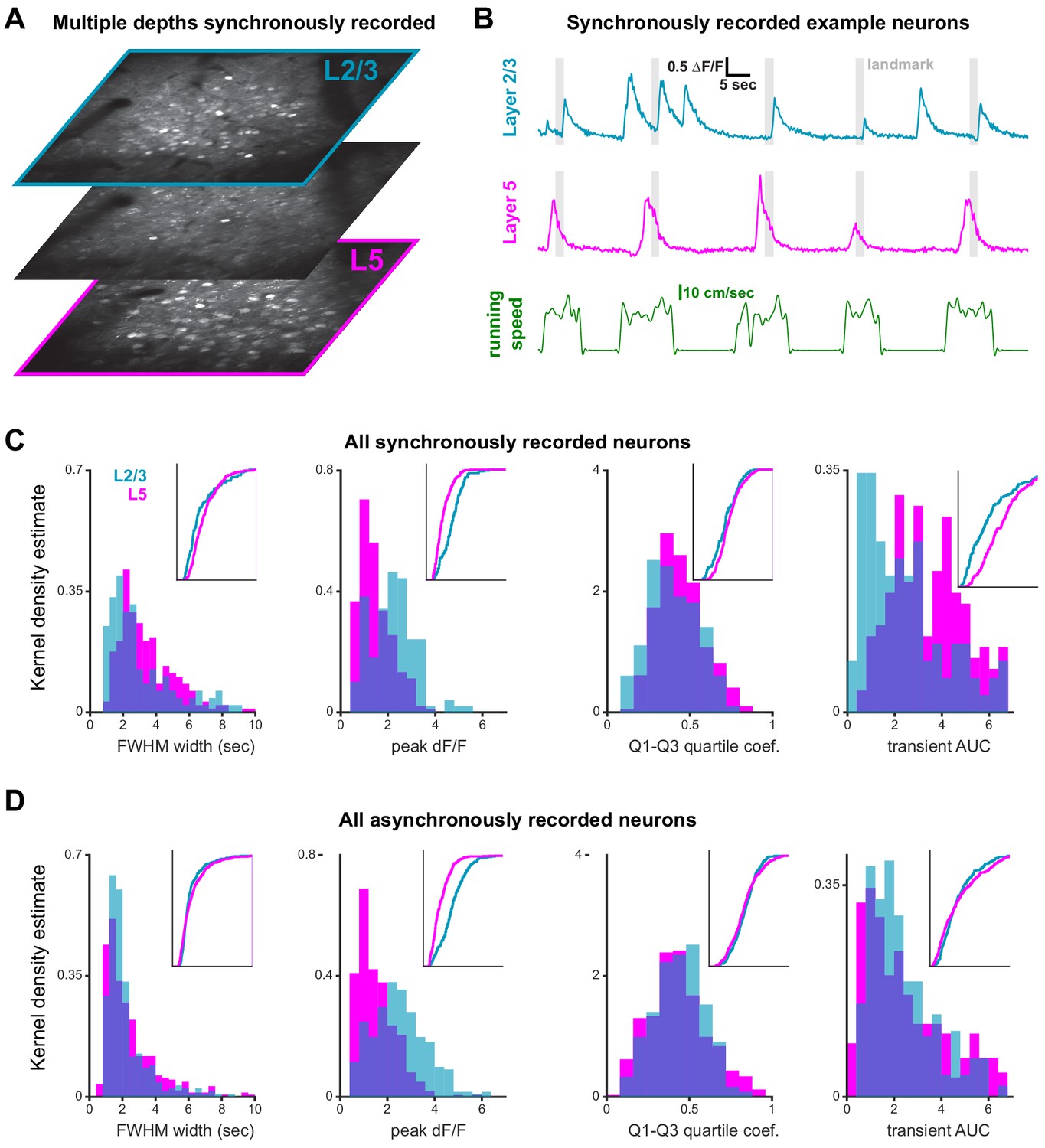
Simultaneous imaging of layer 2/3 and 5.
(A) Mean images of layers 2/3, 5, and an intermediate imaging plane (3 out of a total of 6). Note the almost total lack of cell bodies in the intermediate layer. (B) Two example traces and the corresponding running speed. (C) Properties of transients of all simultaneously recorded neurons in L2/3 and L5 neurons (n = 3 sessions from three mice. Note: only one session is included in data of main figures as behavior was below threshold for the other two.). Full width at half maximum (FWHM), Q1-Q3 quartile coefficient of peak amplitudes, and area under the curve (AUC) were broadly similar. Only peak ∆F/F differed between layers, which is likely explained by differences in optical access to superficial vs deep layers. (D) Same data as in (C) but this time from asynchronously recorded neurons (n = 7 sessions from five animals, all included in main figures). Properties for synchronously and asynchronously recorded neurons are broadly similar; only AUC differs, which may be explained by the impact stray fluorescence from overlaying GCaMP6f expression neurons.
Figure 3 with 1 supplement
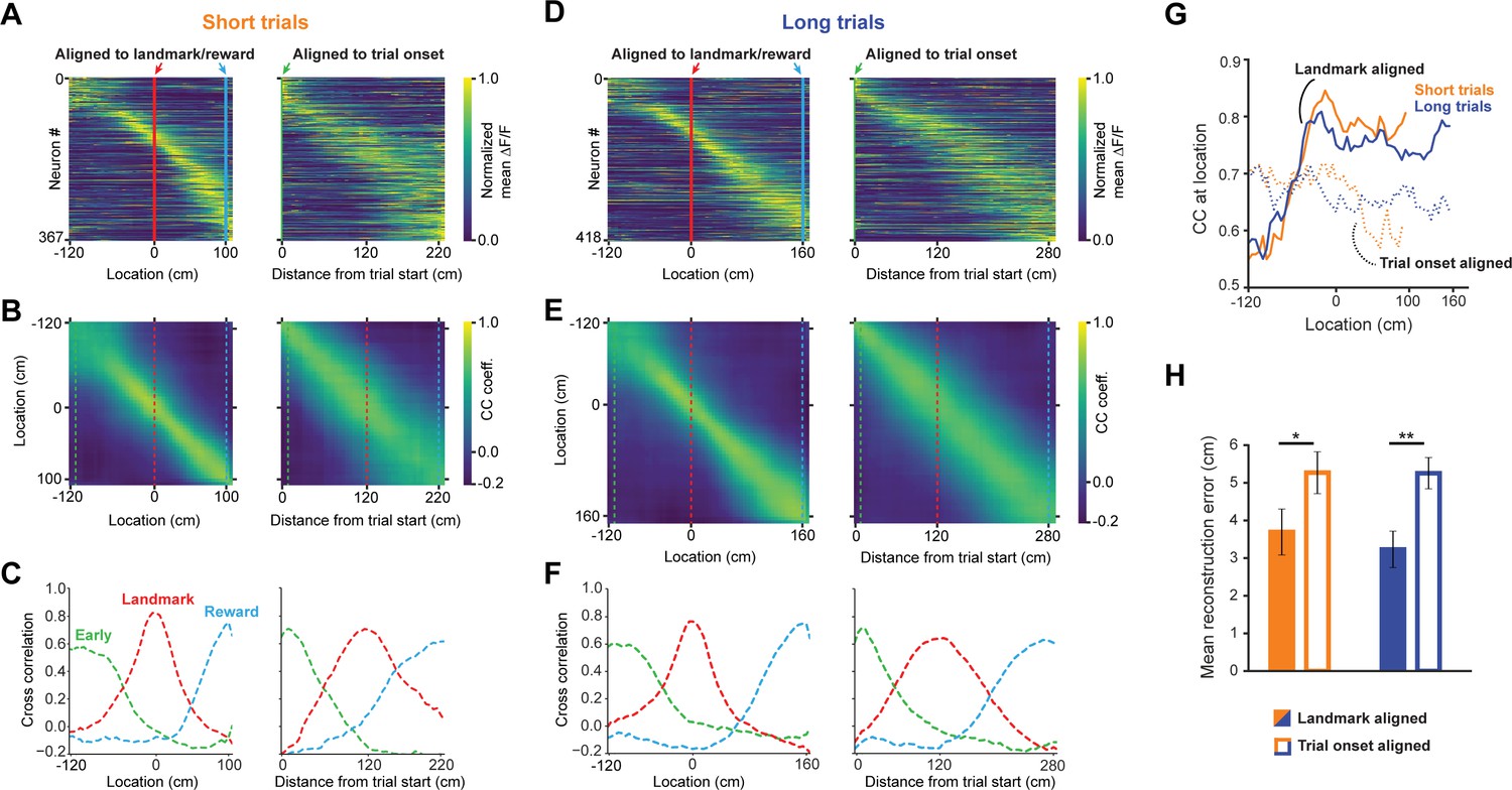
A landmark-anchored code for space in RSC.
(A) Activity of all task engaged neurons ordered by location of peak activity on short trials. Left columns: neurons aligned to the landmark/reward; right columns: same neurons aligned to trial onset point. (B) Population vector cross-correlation matrices of data shown in (A). (C) Slices of the cross-correlation matrices early on the track (green dashed line), at the landmark (red dashed line), and at the reward point (blue dashed line), show sharpening of the spatial code at the landmark. (D–F) Same as (A–C) but for long trials. (G) Population vector cross-correlation values at the animal’s actual location. Solid lines: activity aligned to landmark/reward; dashed lines: activity aligned to trial onset. (H) Reconstruction error, calculated as the mean distance between the maximum correlation value in the cross-correlation matrices and the animal’s actual location, is significantly lower when neural activity is aligned to landmarks (solid bars) compared to trial onset aligned (open bars; Mann-Whitney U: short trials: p<0.05, long trials: p<0.001).
Figure 3—figure supplement 1

Short track and long track neurons activity on opposite tracks.
(A) Activity of short track neurons on the short track (left), long track (middle) and the cross correlation of population vectors on each track (right). (B) Same as (A) but with long track neuron population. (C) Venn diagram showing the overlap of neural populations. The majority of neurons is active on both tracks with only a small fraction being active on exclusively one or the other. (D) Location reconstruction error using only short track or long track neurons on the respective opposite track is slightly, but not significantly larger compared to the same track (mean reconstruction errorshort/short: 3.04 ± 0.55, errorshort/long: 3.75 ± 3.75; error long/long: 2.93 ± 0.44, error long/short: 4.22 ± 0.65; unpaired t-test short track active neurons: p=0.39, long track active neurons: p=0.1). (E) Stacked bar chart trial type selectivity index [(Responseshort – Responselong)/(Responseshort + Responselong)] for all three cell types.
Figure 4 with 2 supplements
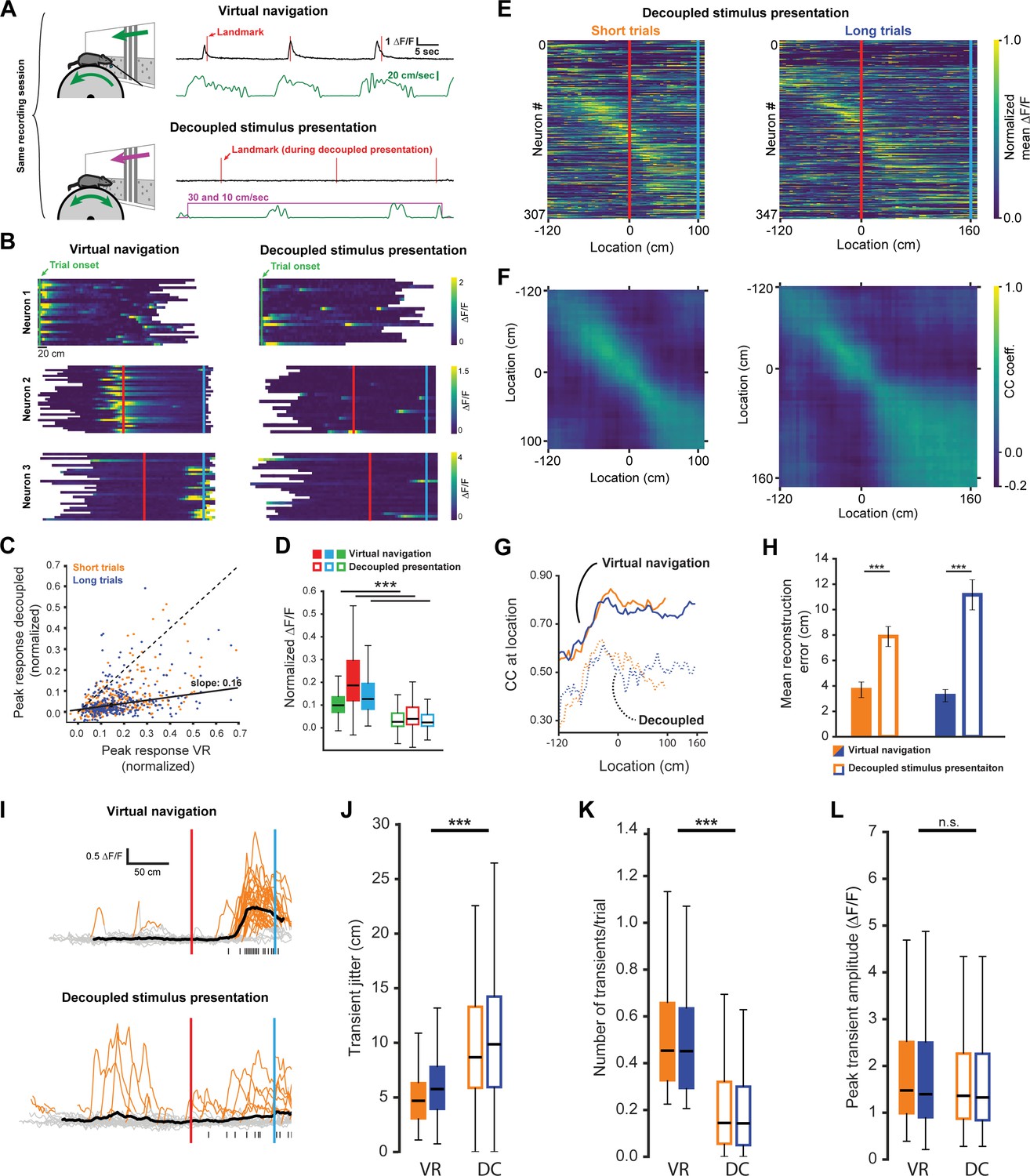
Neuronal activity during decoupled stimulus presentation.
(A) Recording session structure: after recording from neurons during virtual navigation, the same stimuli were presented in an ‘open loop’ configuration where the flow speed of the virtual environment was decoupled from the animal’s movement on the treadmill. (B) Trial onset, landmark, and reward example neurons under these two conditions. (C, D) Response amplitudes of all task engaged RSC neurons during decoupled stimulus presentation (Kruskal-Wallis: p<0.0001, Wilcoxon signed-rank pairwise comparison with Bonferroni correction indicated in (D)). (E, F) Population activity and population vector cross-correlation during decoupled stimulus presentation for short (left) and long (right) trials. (G) Local cross-correlation at animal’s location is smaller during decoupled stimulus presentation. (H) Mean location reconstruction error. Reconstructing animal location from population vectors is significantly less accurate when the animal is not actively navigating (unpaired t-test, short trials and long trials: p<0.0001). (I) Traces of example neuron activity overlaid during virtual navigation (top) and decoupled stimulus presentation (bottom) with transients highlighted in orange. Ticks along bottom indicate peaks of transients around the neuron’s peak response. (J) Spread of transient peak location around peak mean response measured as the standard error of the mean of (standard error of mean of transient peak location – mean peak location). Solid bars: virtual navigation (VR), open bars: decoupled stimulus presentation (DC). (K) Average number of transients/trial during virtual navigation and decoupled stimulus presentation. (L) Average amplitude of transients in VR and DC conditions. Boxplots show median, 1st - 3rd quartile, and 1.5 interquartile range.
Figure 4—figure supplement 1
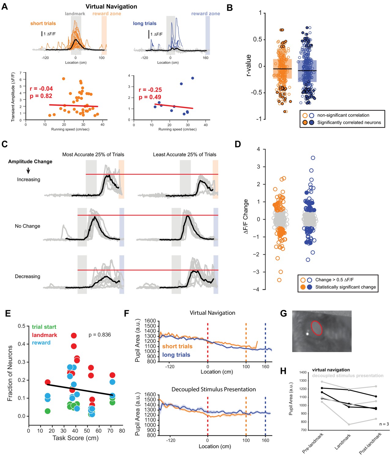
Neural correlates of running speed and reward location prediction.
(A) Top: Example neuron activity as a function of space. Bottom: Peak transient amplitude as a function of running speed with the slope of a fitted regression line shown in red. (B) R-values of linear regression fit for all neurons with at least 10 transients on a given trial type. Neurons that show significant correlation are highlighted. (C) Three examples of neurons increasing, decreasing or not changing activity based on the most vs. the least accurate 25% of trials. (D) Changes in ∆F/F between most and least accurate 25% of trials showing a subset of neurons changing their amplitude, some of which significantly depending on how well an animal predicted the location of the reward (n = 736 task active neurons, n = 159 neurons with a ∆F/F change > 0.5, 28 neurons with a significant change in ∆F/F (two-tailed T-test of transient amplitudes)). (E) Correlation between task score and fraction of neurons aligned to trial onset, landmark and reward (Pearson correlation, p = 0.836). (F) Example pupil dilation as a function of location on the track during active navigation and decoupled stimulus presentation. (G) Example frame showing the pupil illuminated by the 2-photon laser. Red ring indicates the pupil detection from which the pupil area was calculated. (H) Pupil dilation before, at, and after the landmark showing no significant difference (pre-landmark: 0–100 cm before landmark, post-landmark: end of landmark to start of reward zone, one-way ANOVA: p = 0.66).
Figure 4—figure supplement 2

Stable long-term imaging.
(A) Raw brightness data from one example ROI (gray, top) and whole field-of-view (FOV) brightness (red, bottom) during virtual navigation (left) and subsequent decoupled stimulus presentation (right). Dashed lines across red traces are linear regression fits. (B) Mean frame brightness of all frames during virtual navigation and decoupled stimulus presentation. (C) Regression line slopes of all ROIs in FOV from which examples are shown in (A) and (B). (D) Regression line slopes of FOVs for all recording sessions of RSC neurons contained in this study.
Figure 5

Non-linear integration of visual and motor inputs in RSC landmark neurons.
(A) Example neuron during virtual navigation (top) and decoupled stimulus presentation as the animal is running or resting (bottom). (B) Same neuron as in (A) with all instances where the animal was running or resting, averaged (left) and raster plots of the whole session (right). Peak mean activity indicated by dashed blue line. (C) Activity of population during virtual navigation and decoupled stimulus presentation (D) Neuronal responses normalized to peak activity in VR under different conditions. ‘No input’ and ‘motor only’ responses were measured while animals are in the black box between trials (median and spread of data shown in (C)). (E) The sum of ‘landmark, no motor’ + ‘motor’ is smaller than ‘landmark + motor’ responses suggesting nonlinear combination of visual and motor inputs. (Wilcoxon signed-rank test, p<0.01). (F) Traces of example neuron when the animal is passively watching the scene (top) or locomoting (bottom). Black ticks along bottom indicate transients around that neuron’s peak mean activity during virtual navigation (see Figure 4I). (G) Spread of transient location around peak mean activity in VR (standard error of mean of transient peak location – mean peak location). (H) Average number of transients/trial and (I) average amplitude in both conditions. Kruskal-Wallis test p<0.0001; Mann-Whitney-U pairwise comparisons with Bonferroni correction results indicated, * = <0.05, ** = <0.01, *** = <0.001. Boxplots show median, 1st - 3rd quartile, and 1.5 interquartile range.
Figure 6

Neural activity in naive and expert animals.
(A) Example field of views in the naïve (left) and expert (right) mouse with neurons that are shown in (B). Naïve mice were exposed to the virtual track for the first time after being previously habituated to being head restrained and running on a treadmill as well as receiving rewards at pseudo-random intervals. (B) Two example neurons that modified their activity as a function of training. Neuron 1 (top) showed no discernable receptive field in the naïve animal. However, in the expert animal, it showed a clear receptive field after the landmark. Neuron 2 (bottom) in contrast, showed some landmark-anchored activity that was strongly amplified in the expert condition. (C) Activity of task-active neurons in expert animals shown in both naïve and expert sessions (n = 81 short track, 80 long track). (D) Population vector cross-correlation matrix of activity in naïve and expert sessions. (E) Cross correlation value of population vectors at the actual location of the animal in naïve and expert sessions calculated from task active neurons in the respective sessions. (F) Reconstruction error in naïve and expert conditions (mean ± SEM reconstruction error short/long: 2.07 ± 0.37/2.67 ± 0.46 (expert), 5.1 ± 0.63/5.7 ± 0.62 (naive); two tailed t-test, short and long: p<0.001).
Figure 7 with 1 supplement
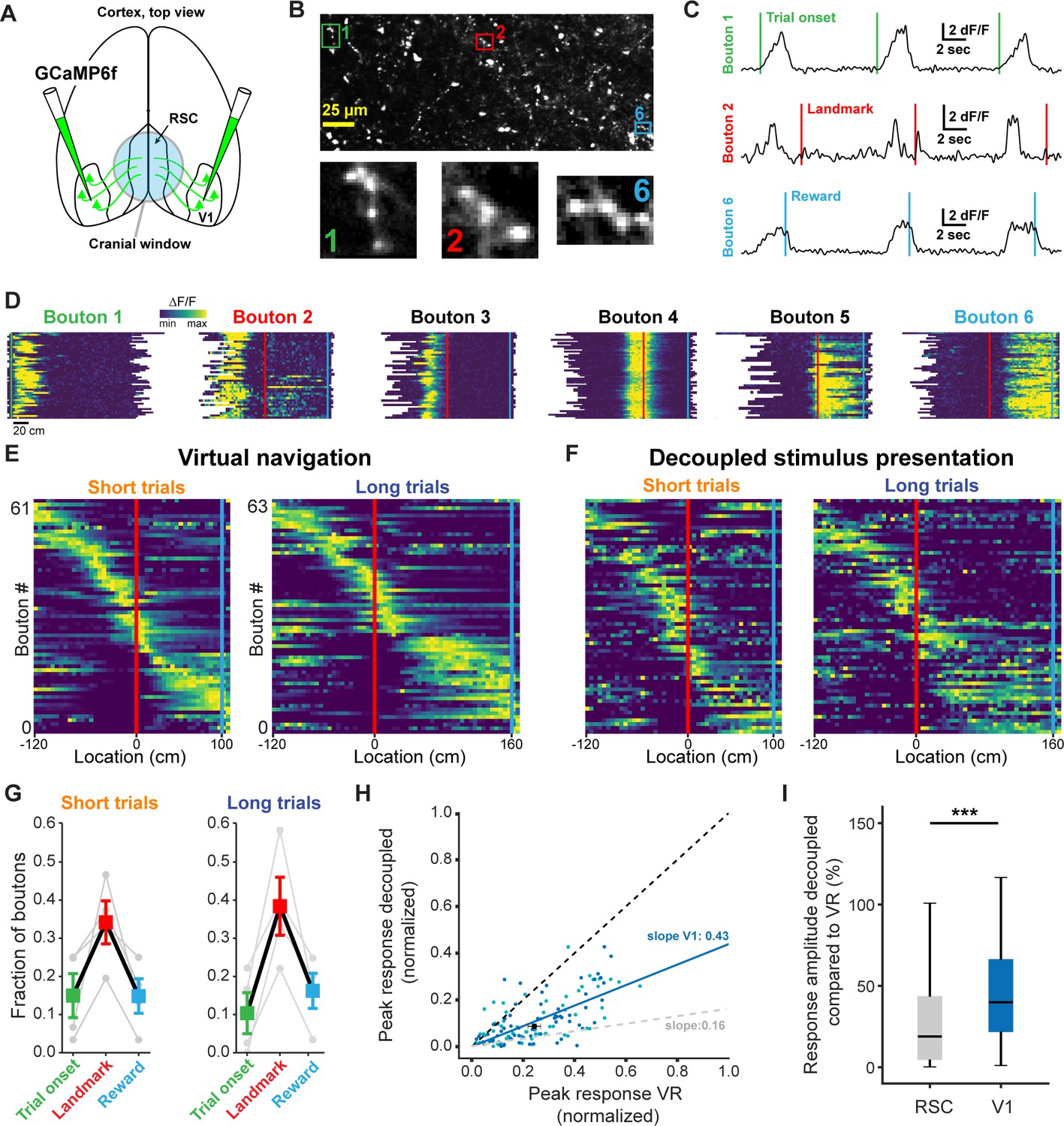
V1 axonal bouton responses in RSC.
(A) Overview of injection and recording site. (B) Example FOV and three example boutons shown in (C) and (D). Where possible, ROIs were drawn around clusters of boutons belonging to the same axon. (C) Trial onset, landmark, and reward aligned boutons from same animal. (D) Six example boutons showing tuning to pre- and post-landmark portions of the track. (E) Population of V1 boutons in RSC ordered by location of their response peak (n = 61 boutons short track/63 boutons long track, four mice). (F) Same boutons as in (E) during decoupled stimulus presentation. (G) Alignment of boutons to task features. (H) Response amplitude during virtual navigation of decoupled stimulus presentation with fitted regression line. In gray: fitted regression line for RSC neurons. (I) Comparison of response amplitude differences between VR and decoupled stimulus presentation in RSC neurons and V1 boutons (meanRSC = 0.42 ± 0.03, meanV1 = 0.53 ± 0.04, Mann-Whitney U test: p<0.001).
Figure 7—figure supplement 1
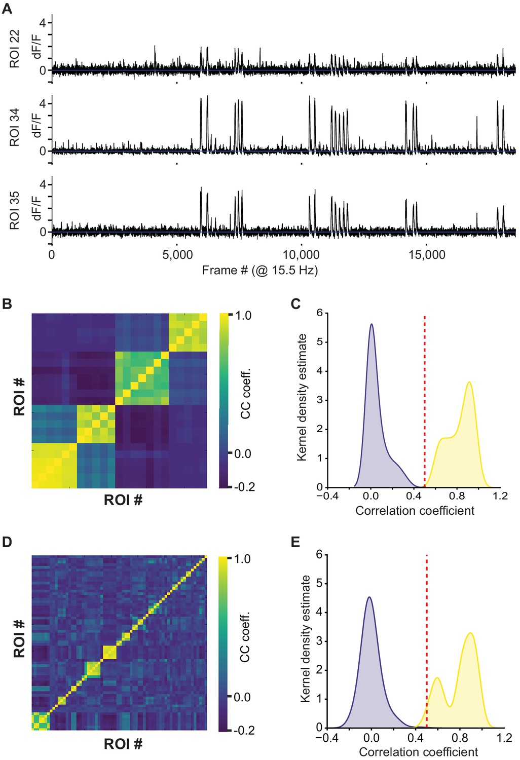
Identification process for unique axonal inputs.
(A) Traces of three bouton ROIs, putatively from the same axon. (B) Cross-correlation matrix of 23 boutons, manually identified to belong to four individual axons. (C) Cross-correlation of all boutons in (B), split into those belonging to the same axon (yellow) and different axons (blue). The threshold was set manually at 0.5 based on this distribution. (D) The cross-correlation matrix was ordered by grouping together all ROIs above the threshold estimated in (C). (E) Same plot as (C). Confirmation that the threshold in (C) is valid for the whole population.
Author response image 1
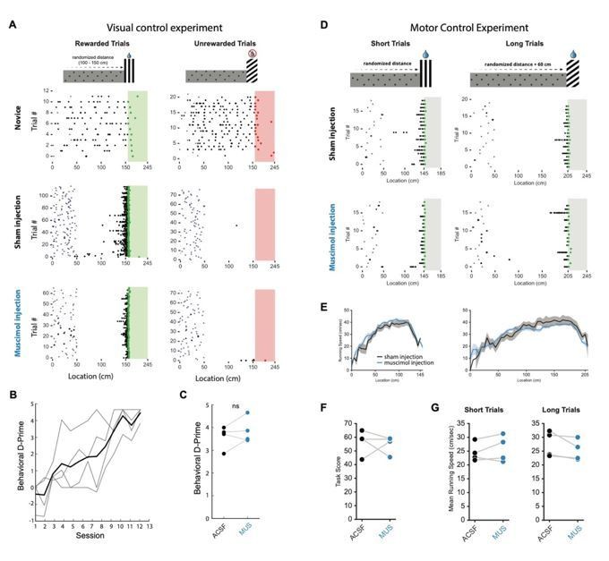
Muscimol inactivation on visual discrimination and motor control tasks.
(A) Schematic of visual discrimination task (top) in which reward was available at one visual cuebut not the other. The distance to both visual cues was equal. Animals learned to discriminate reliably (middle raster plot) and task performance was not affected by multi-site (2-4) bilateral muscimol injections into RSC A30 (bottom raster plot). (B) Behavioral D-Prime showing that all animals learned the task in ~10-12 sessions (n=4 mice). (C) D-Prime during sham and muscimol injections. (D) Top: schematic of motor control experiment where animals ran different distances to obtain rewards at either visual cue. On the short trials, mice had to travel an average of 140 cm while on the long trials they had to travel 200 cm on average. Both visual cues were rewarded. Raster plots show behavior during sham and muscimol multisite bilateral injection into RSC A30. (E,G) Running speed profiles and mean running speeds during sham and muscimol injection. (F) Task score during sham and muscimol injection.
Additional files
-
Source code 1
Analysis code.
- https://cdn.elifesciences.org/articles/51458/elife-51458-code1-v1.zip
-
Transparent reporting form
- https://cdn.elifesciences.org/articles/51458/elife-51458-transrepform-v1.docx
Download links
A two-part list of links to download the article, or parts of the article, in various formats.
Downloads (link to download the article as PDF)
Open citations (links to open the citations from this article in various online reference manager services)
Cite this article (links to download the citations from this article in formats compatible with various reference manager tools)
Representation of visual landmarks in retrosplenial cortex
eLife 9:e51458.
https://doi.org/10.7554/eLife.51458


