The cellular architecture of memory modules in Drosophila supports stochastic input integration
- Zanvyl Krieger Mind/Brain Institute, Johns Hopkins University, United States
- Division of Neurobiology and Zoology, Department of Biology, University of Kaiserslautern, Germany
- Physiology of Neuronal Networks Group, Department of Biology, University of Kaiserslautern, Germany
- Solomon Snyder Department of Neuroscience, Johns Hopkins University, United States
Figures
Figure 1 with 2 supplements
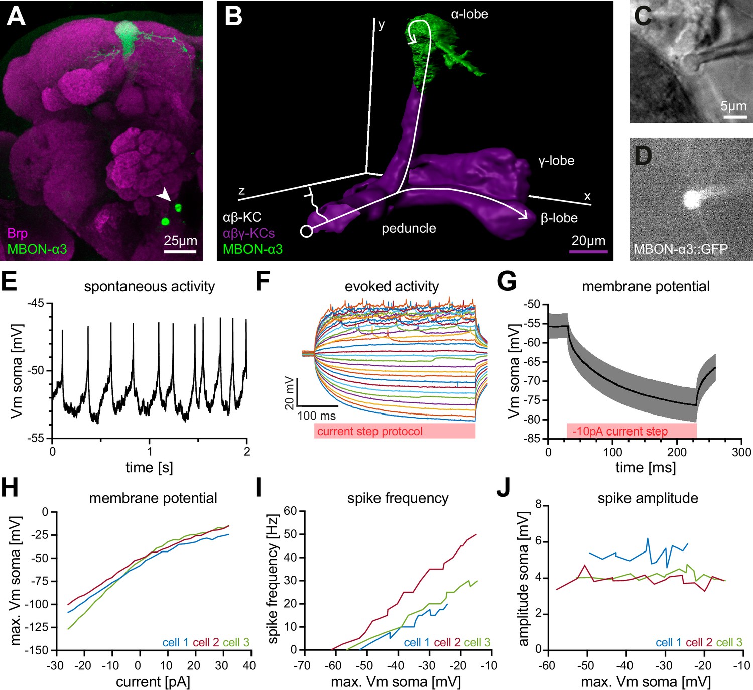
Electrophysiological characterization of the MBON-α3 neuron.
(A) Immunohistochemical analysis of the MBON-α3 (green, marked by GFP expression) reveals the unique morphology of the MBON with its dendritic tree at the tip of the α-lobe and the cell soma (arrowhead) at a ventro-medial position below the antennal lobes. The brain architecture is revealed by a co-staining with the synaptic active zone marker Bruchpilot (Brp, magenta). (B) Artificial superimposition of a partial rendering of MBON-α3 (green) and of -KCs (magenta) to illustrate KC>MBON connectivity. A simplified schematic -KC projection is illustrated in white. (C) Transmitted light image of an MBON-α3 cell body attached to a patch pipette. (D) Visualisation of the GFP-expression of MBON-α3 that was used to identify the cell via fluorescence microscopy. The patch pipette tip is attached to the soma (right side). The scale bar in C applies to C and D. (E) Recording of spontaneous activity of an MBON-α3 neuron in current clamp without current injection. (F) Recording of evoked neuronal activity of an MBON-α3 neuron with step-wise increasing injection of current pulses. Pulses start at (bottom) with increasing steps and end at (top). (G) Mean trace of the induced membrane polarization resulting from a long current injection of . 105 trials from three different cells (35 each) were averaged. Gray shading indicates the SD. (H) Relative change of membrane potential after current injection. Vm is equal to the maximum depolarization of the membrane. (I) Correlation between the frequency of action potential firing and changes in membrane potential. (J) Relative change of spike amplitude after current injections. Spike amplitude represents the peak of the largest action potential minus baseline. Also see Figure 1—figure supplement 1 and Figure 1—figure supplement 2.
Figure 1—figure supplement 1

Additional information about the electrophysiology of MBON-α3.
Second (A) and third (B) example cells for the evoked neuronal activity of MBON-α3 through a step-wise increasing injection of current pulses. Pulses start at (bottom) with increasing steps and end at (top). (C) Correlation between frequency of action potential firing and injected current. The frequency describes action potentials per second. (D) Relative change of spike amplitude after current injections. Spike amplitude corresponds to the peak of the highest action potential minus baseline. (E) Change of membrane potential relative to the resting membrane potential after current injection. ΔVm is equal to the maximum depolarisation minus the resting membrane potential.
Figure 1—figure supplement 2
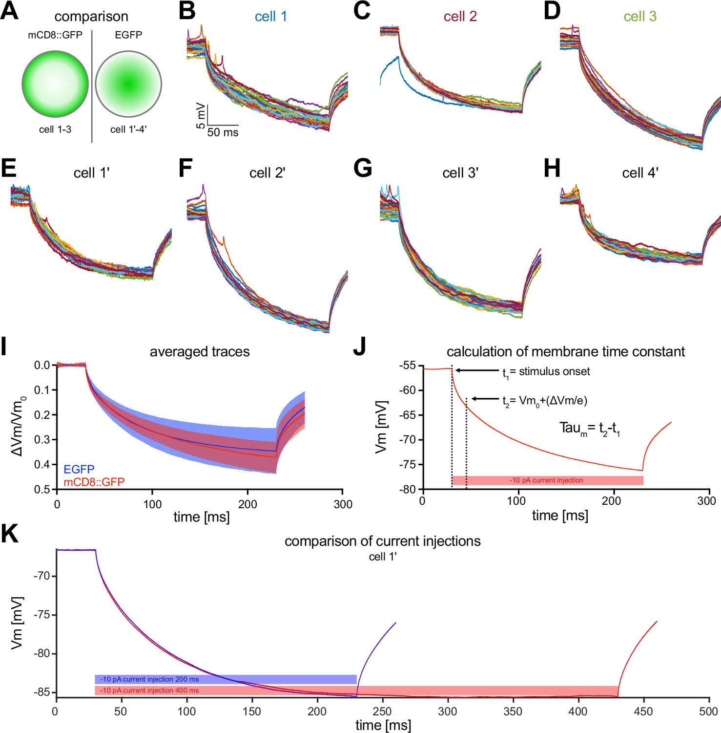
Electrophysiological properties of MBON-α3.
(A) MBON-α3 was identified for patch-clamp recordings using either mCD8::GFP (data in B-D) or cytoplasmic EGFP (data in E-H). (B–H) Raw traces of the induced membrane polarization resulting from a long current injection of . (I) Comparison of the mean traces of the three cells recorded using mCD8::GFP (B-D, red) and the four cells recorded using EGFP (E-H, blue). Blue and red shadings indicate the SD. (J) Exemplary illustration of the procedure to determine the membrane time constant tau. All parameters used to calculate are highlighted. The first vertical dashed line is defined as the time () when the current injection starts. The second line () is when the voltage has decayed to , where is the difference between and the asymptotic voltage, and is the base of the natural logarithm. Thus, at , the deflection is at 1/e of the maximum deflection. (K) Comparison of and current injections of from an example cell (cell 1’). No significant difference for could be detected between the two stimulation protocols.
Figure 2 with 2 supplements
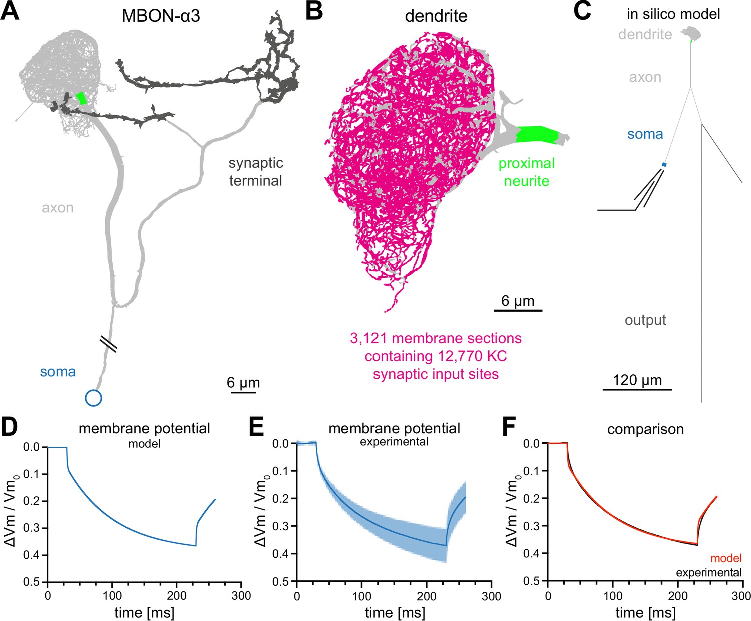
Construction of a computational model of MBON-α3.
(A) Electron microscopy based reconstruction of MBON-α3. Data was obtained from NeuPrint (Takemura et al., 2017) and visualized with NEURON (Hines and Carnevale, 1997). Data set MBON14 (ID 54977) was used for the dendritic architecture (A–C) and MBON14(a3)R (ID 300972942) was used to model the axon (light gray) and synaptic terminal (dark gray, A, C). The proximal neurite (bright green) was defined as the proximal axonal region next to the dendritic tree. This is the presumed site of action potential generation. Connectivity to the soma (blue) is included for illustration of the overall morphology and is not drawn to scale. (B) A magnified side view of the dendritic tree of MBON-α3. Within the dendritic tree a total of 4336 individual membrane sections were defined (light gray area). The 3121 membrane sections that contain one or more of the 12,770 synaptic input sites from the 948 innervating KCs are highlighted in magenta. (C) Simplified in silico model of MBON-α3 highlighting the size of the individual neuronal segments. We simulated recordings at the proximal neurite (specified as the potential site of action potential generation based on morphological parameters; this area is still included in the dendritic tree reconstruction of Takemura et al., 2017) or at the soma. Values for the different sections are provided in Figure 2—figure supplement 1, Figure 2—source data 1. (D) Normalized trace of a simulated membrane polarization after injection of a long square-pulse current of at the soma. (E) Normalized and averaged experimental traces (blue) with standard deviation (light blue) of our measured depolarization. (F) Comparison of a normalized induced depolarization from the model (red) and from the experimental approach (black). The model was fitted within the NEURON environment to the measured normalized mean traces with a mean squared error between model and measured data of . Also see Figure 2—figure supplement 1, Figure 2—figure supplement 2 and Figure 2—source data 1.
-
Figure 2—source data 1
Numerical values of the individual sections of the neuron utillized for the computational model.
- https://cdn.elifesciences.org/articles/77578/elife-77578-fig2-data1-v4.xlsx
Figure 2—figure supplement 1
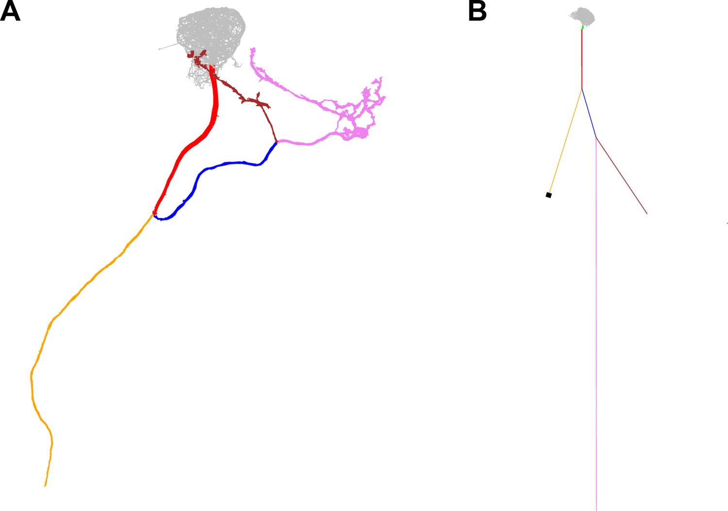
Overview of the axonal sections and soma in the in silico model.
The pink and brown sections represent the presynaptic release sites of MBON-α3. Color-coded electron-microscopy based reconstruction (A) and in silico model (B). The reconstruction of the hemibrain did not include the complete axonal area (yellow) and the soma. (B) illustrates the appended sections and the corresponding diameter and lengths. The soma diameter (black) and axon length (yellow) were estimated from confocal microscopy images and literature. Values of individual segments are presented Figure 2—source data 1.
Figure 2—figure supplement 2

Origin of the fast voltage change followed by slower change subsequent to current steps, visible in Figure 2D, E and F.
We hypothesize that this behavior is a reflection of the cell’s morphology, shown in panel A of that Figure, as well as in Figure 2—figure supplement 1. In the experiment, as well as in the simulation, current is injected into the soma and recorded there. The soma is a relatively small compartment, with small membrane area. It is connected via a long, thin neurite with the rest of the cell which has a substantially larger membrane area. Current injection charges the somatic capacitance very quickly, leading to a rapid change in the somatic voltage at each current step, while the rest of the cell reacts on a much larger time scale. This is visible by the small ‘kink’ right after each change in the injected constant current, Figure 2D. (A) Highly simplified schematic circuit of the cell. The soma is represented by the RC circuit consisting of a resistor and a capacitor. The time constant of this circuit is very short . The neurite connecting it to the rest of the cell (axon and dendrites) is represented by a resistor. The rest of the cell is represented by the second RC circuit ( resistor and capacitor) with a time constant exceeding that of the soma by a factor of ten. (B) Simulated current step protocol in the simplified circuit, with negative current injected for and then removed (red bar). The somatic voltage (green trace) shows the fast change at start and end of the current injection, followed by a slower near-exponential trace. This Link to the circuit simulator allows the reader to simulate the circuit shown in (A). Closing the switch, by clicking on its symbol, starts the current injection and shows the soma voltage, that is the voltage over the capacitor. Opening the switch (by clicking on the symbol again) results in the circuit returning to its equilibrium state. The voltage trace (green) displays the two characteristic times of the coupled circuit. To ensure long-term access to the circuit simulation, we captured a web archive snapshot of the web app. (C) The two time scales are visible in the electrophysiologically recorded raw (not averaged) voltage, in fact more clearly than in the averaged data in Figure 2D, E and F. Shown here are two representative voltage traces recorded from cell 1 in Figure 1—figure supplement 2B.
Figure 3 with 1 supplement
Computational characterization of MBON-α3.
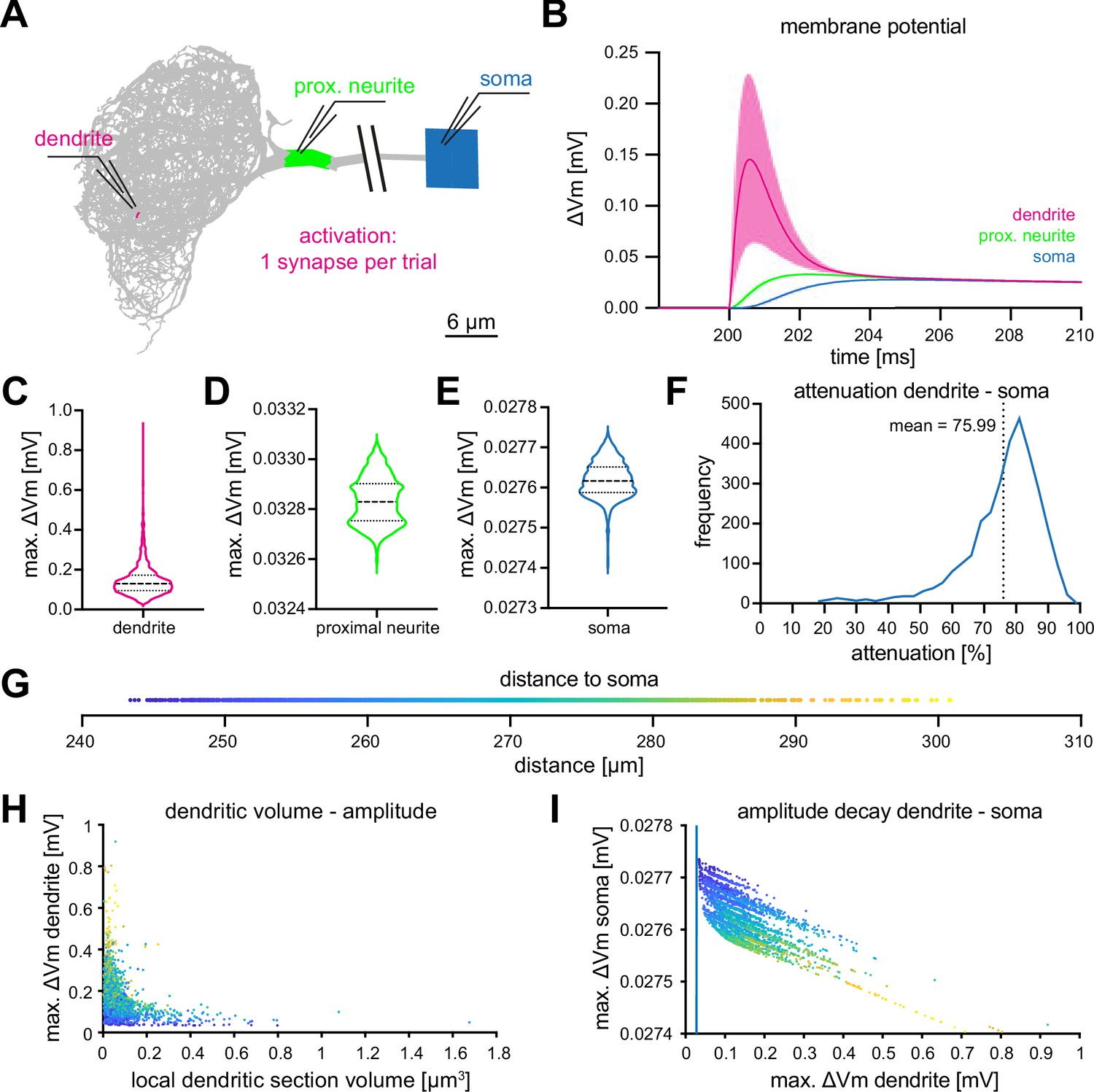
(A) Simulated stimulation of individual synaptic input sites. Voltage deflections of synaptic currents were analyzed locally at the dendritic segment (red, next to electrode tip), the proximal neurite (green) and the soma (blue). The soma is depicted as a square that reflects its size in the NEURON environment. Color code also applies to B-F. (B) Resulting mean voltages (lines) and standard deviations (shading) from synaptic activations in 3121 individual stimulus locations (dendrite), and at the proximal neurite and soma. (C–E) Violin plots of the simulated maximal amplitudes at the dendritic section (C), the proximal neurite (D) and the soma (E) in response to synaptic activations. Dotted lines represents the quartiles and dashed lines the mean. Proportions of the violin body represent the distribution of individual data points. Note the difference in scale and compactification of the amplitudes in the proximal neurite and soma. (F) Distribution of the percentage of voltage attenuation recorded at the soma. (G) Distribution of distance between all individual dendritic sections and the soma. This color code is applied in H and I. (H) The elicited local dendritic depolarization is plotted as a function of the local dendritic section volume. (I) The soma amplitude is plotted as a function of the amplitude at individual dendritic segments. Note different scales between abscissa and ordinate; the blue line represents identity. Also see Figure 3—figure supplement 1.
Figure 3—figure supplement 1
Additional information about voltage attenuation at the proximal neurite and soma.
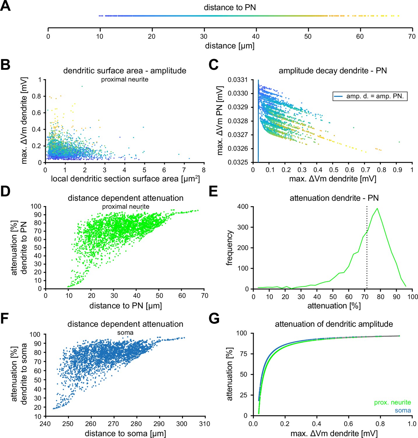
(A) Distance to the proximal neurite for each stimulated dendritic segment with the color code for the following graphs. (B) Scatter plot of the elicited amplitude relative to the resting membrane potential in each stimulated dendritic section as function of its surface area. (C) Scatter plot of the voltage in the proximal neurite as a function of the voltage in the dendrite, both relative to their baseline values. The blue line represents the line of identity. (D) Correlation of the measured distance to the proximal neurite with the percent of voltage attenuation in the proximal neurite for each synaptic section. (E) Distribution of the percentage of voltage attenuation in the PN per synapse. Vertical dotted line represents the mean attenuation in percent. (F) Correlation of the measured distance to the soma with the percent of voltage attenuation in the soma for each synaptic section. (G) Correlation of the attenuation in percent at the soma (blue) or at the proximal neurite (green) relative to the dendritic voltage.
Figure 4
MBON-α3 is electrotonically compact.
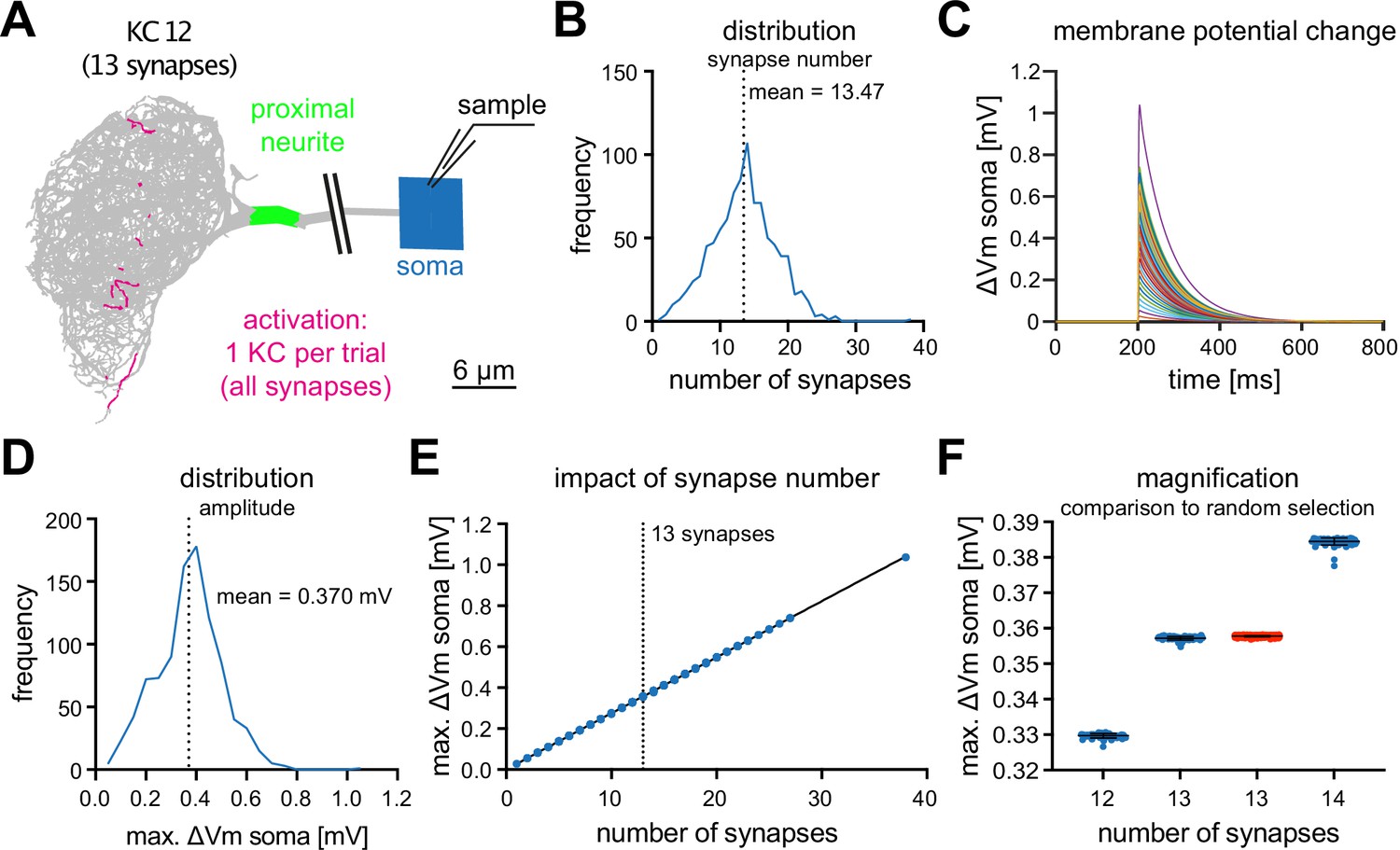
(A) Simulated activation of all synapses from all 948 individual KCs innervating MBON-α3. A representative example of a KC (KC12) with 13 input synapses to MBON-α3 is shown. (B) Histogram of the distribution of the number of synapses per KC. (C) Membrane potential traces from simulated activation of all 948 KCs. (D) Distribution of the elicited amplitudes evoked by the individual activations of all KCs. (E) Correlation between the somatic amplitude and the number of activated synapses in the trials. (F) Blue: Distribution of the somatic voltage change evoked by the activation of all KCs with exactly 12, 13, or 14 input synapses. Each dot represents one simulated KC. Bars represent mean and SD. Red: Same, but for activation of 13 random synapses per simulation in 1000 independent trials.
Figure 5
Effect of KC recruitment and synaptic plasticity on MBON-α3 responses.
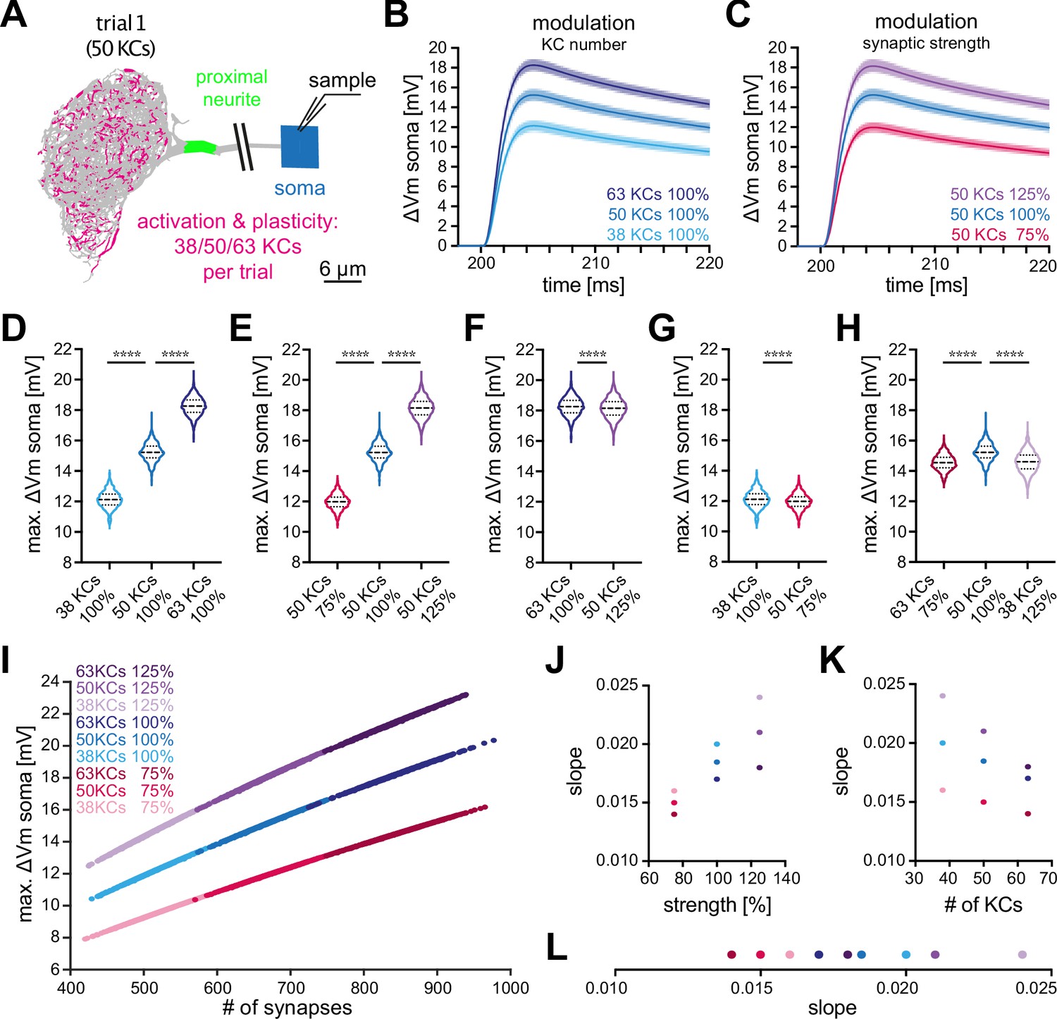
(A) Schematic of the simulated recording paradigm. We modeled the activation of ≈5% of random combinations of identified KCs, that is we activated the anatomically correct synapse locations of 50 randomly selected KCs to mimic activation by an odor. The panel shows the distribution of activated synapses for one of these trials. We then varied the number of activated KCs by ±25% around its mean of 50, that is 38, 50, and 63 KCs, and we varied synaptic strength ±25% around its original value, that is 75%, 100%, and 125%. (B) Mean somatic depolarizations after activating 1000 different sets of either 38 (light blue), 50 (blue), or 63 (dark blue) KCs, all at standard synaptic strength (100%). Shades represent the standard deviations. (C) Mean somatic depolarizations after activating 1000 different sets of 50 KCs at either 75% (red), 100% (blue), or 125% (purple) synaptic strength. Shades represent the standard deviations. (D, E) Violin plots of the relative amplitudes evoked by the different KC sets from (B, C). (F–G) Violin plots for the comparison of the amplitudes between the different plasticity paradigms. (F) 63 KCs at 100% vs 50 KCs at 125% synaptic strength. (G) 38 KCs at 100% vs 50 KCs at 75% synaptic strength. Plots in D-G use the color code from (B) and (C). (H) 63 KCs at 75% (dark red) vs. 50 KCs at 100% (blue) and 38 KCs at 125% (light purple) synaptic strength. See Figure 3 for symbols in violin plots. (I) Relation between somatic depolarization and the number and strength of activated synapses. Illustrated are all tested conditions for synaptic plasticity and KC recruitment. Stimulation paradigms are color coded as shown. (J) Relation between the slope of the condition-specific linear regressions from (I) and the synaptic strength of the activated KC sets. (K) Relation between the slope of the condition-specific linear regressions from (I) and the number of recruited KCs. (L) Slopes of the condition-specific linear regressions from (I). Color codes of (J–L) as in (I). Statistical significance was tested in multiple comparisons with a parametric one-way ANOVA test (D, E and H) resulting in p=<0.0001 for all conditions, or in an unpaired parametric t-test (F and G) resulting in p=<0.0001 for all conditions. Numerical results are summarized in Table 3.
Author response image 1

Simplified circuit of a small soma (left parallel RC circuit) and the much larger remainder of a cell (right parallel RC circuit) connected by a neurite (right 100MΩ resistor).
A current source (far left) injects constant current into the soma through the left 100MΩ resistor.
Author response image 2

Somatic voltage in the circuit in Figure 1 with current injection for about 4.
5ms, followed by zero current injection for another ≈ 3.5ms..
Author response image 3

: Somatic voltage in the circuit, as in Figure 2 but with current injected for approx.
15ms.
Author response image 4

Somatic voltage in the circuit, as in Figure 2 but showing only for the time right after current onset, about 2.
3ms.
Tables
Table 1
Summary of passive membrane properties of MBON-α3, calculated from electrophysiological measurements from five neurons.
| Sample | |||||
|---|---|---|---|---|---|
| Cell 1 | –59.2 | 13.54 | 12.35 | 0.200 | 1.87×10⁻⁵ |
| Cell 2 | –52.3 | 14.46 | 20.79 | 0.337 | 2.12×10⁻⁵ |
| Cell 3 | –56.2 | 24.58 | 21.60 | 0.350 | 1.48×10⁻⁵ |
| Cell 4 | –52.8 | 15.50 | 15.83 | 0.257 | 1.66×10⁻⁵ |
| Cell 5 | –63.1 | 12.20 | 13.21 | 0.214 | 1.76×10⁻⁵ |
| Mean | –56.7 | 16.06 | 16.76 | 0.272 | 1.78×10⁻⁵ |
| SD | 4.5 | 4.92 | 4.26 | 0.069 | 0.24×10⁻⁵ |
| SEM | 2.0 | 2.20 | 1.90 | 0.031 | 0.11×10⁻⁵ |
-
Table 1—source data 1
Summary of the passive membrane properties of MBON-α3, calculated from electrophysiological measurements from four neurons marked by cytoplasmic EGFP.
- https://cdn.elifesciences.org/articles/77578/elife-77578-table1-data1-v4.xlsx
Table 2
Electrophysiological values applied for the in silico model of MBON-α3-A.
Parameter values were obtained from literature or were based on the fitting to our electrophysiological data. The first column shows the parameters, with the names used in the NEURON environment in parentheses. The maximal conductance was determined to achieve the target MBON depolarization from monosynaptic KC innervation.
| Electrophysiological Properties | |||
|---|---|---|---|
| Variable | Description | Fitted | Literature |
| (Ra) | Cytoplasm resistivity [] | 85.41 | 30–400 (Borst and Haag, 1996; Gouwens and Wilson, 2009) |
| (cm) | Specific membrane capacitance [] | 0.6961 | 0.6–2.6 (Borst and Haag, 1996) |
| (pas.g) | Passive membrane conductance [] | (Cassenaer and Laurent, 2007) | |
| (pas.e) | Leak reversal potential [] | –55.64 | –60 (Berger and Crook, 2015) |
| Synaptic Parameters | |||
| (tau) | Time to max. conductance [] | N.A. | 0.44 (Su and O’Dowd, 2003) |
| E | Synaptic current reversal potential [] | N.A. | 8.9 (Su and O’Dowd, 2003) |
| (gmax) | Maximal conductance [ ] | N.A. | (Hige et al., 2015b) |
Table 3
Summary of data from the plasticity simulations of Figure 5.
Simulations vary the number of active KCs and/or the strength of the KC-MBON synapses by scaling the maximal conductance parameter of the synaptic alpha-conductance function. Results include the mean number of activated synaptic sites as well as the mean amplitude of the somatic voltage depolarization across the 1000 trial repetitions of each simulation. Ranges are reported as parentheticals. The slope of the linear regression describing the relation between the number of active synapses and somatic voltage amplitude is reported (Figure 5I–L).
| Simulation parameters | Results | |||
|---|---|---|---|---|
| # KCs | Synaptic strength | Mean # Activated synapses | Mean somatic depolarization amplitude [] | Slope |
| 63 | 125% | 847.88 (747 - 939) | 21.55 (19.66–23.21) | 0.0184 |
| 50 | 125% | 672.55 (573 - 778) | 18.14 (15.99–20.29) | 0.0209 |
| 38 | 125% | 511.77 (425 - 615) | 14.60 (12.48–16.96) | 0.0235 |
| 63 | 100% | 847.08 (725 - 977) | 18.26 (16.15–20.34) | 0.0166 |
| 50 | 100% | 673.76 (574 - 805) | 15.24 (13.34–17.58) | 0.0185 |
| 38 | 100% | 512.48 (429 - 599) | 12.14 (10.43–13.85) | 0.0203 |
| 63 | 75% | 849.05 (749 - 965) | 14.56 (13.11–16.17) | 0.0141 |
| 50 | 75% | 672.86 (570 - 767) | 11.98 (10.37–13.41) | 0.0153 |
| 38 | 75% | 511.97 (420 - 606) | 9.44 (7.91–10.96) | 0.0164 |
Table 4
Morphological parameters of the model.
| Parameter | Value |
|---|---|
| Number of sections | 4342 |
| Average section length | |
| Total length | |
| Average diameter | |
| Average segment surface area | |
| Total surface area | |
| Soma diameter |
Additional files
Download links
A two-part list of links to download the article, or parts of the article, in various formats.
Downloads (link to download the article as PDF)
Open citations (links to open the citations from this article in various online reference manager services)
Cite this article (links to download the citations from this article in formats compatible with various reference manager tools)
The cellular architecture of memory modules in Drosophila supports stochastic input integration
eLife 12:e77578.
https://doi.org/10.7554/eLife.77578


