Normative decision rules in changing environments
- Department of Applied Mathematics, University of Colorado Boulder, United States
- Department of Neuroscience, University of Pennsylvania, United States
- Department of Mathematics, University of Houston, United States
Figures
Figure 1
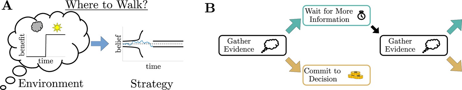
Simple decisions may require complex strategies.
(A) When choosing where to walk, environmental fluctuations (e.g., weather changes) may necessitate changes in decision bounds (black line) adapted to changes in the conditions (cloudy to sunny). (B) Schematic of a dynamic programming. By assigning the best action to each moment in time, dynamic programming optimizes trial-averaged reward rate to produce the normative thresholds for a given decision.
Figure 2 with 3 supplements
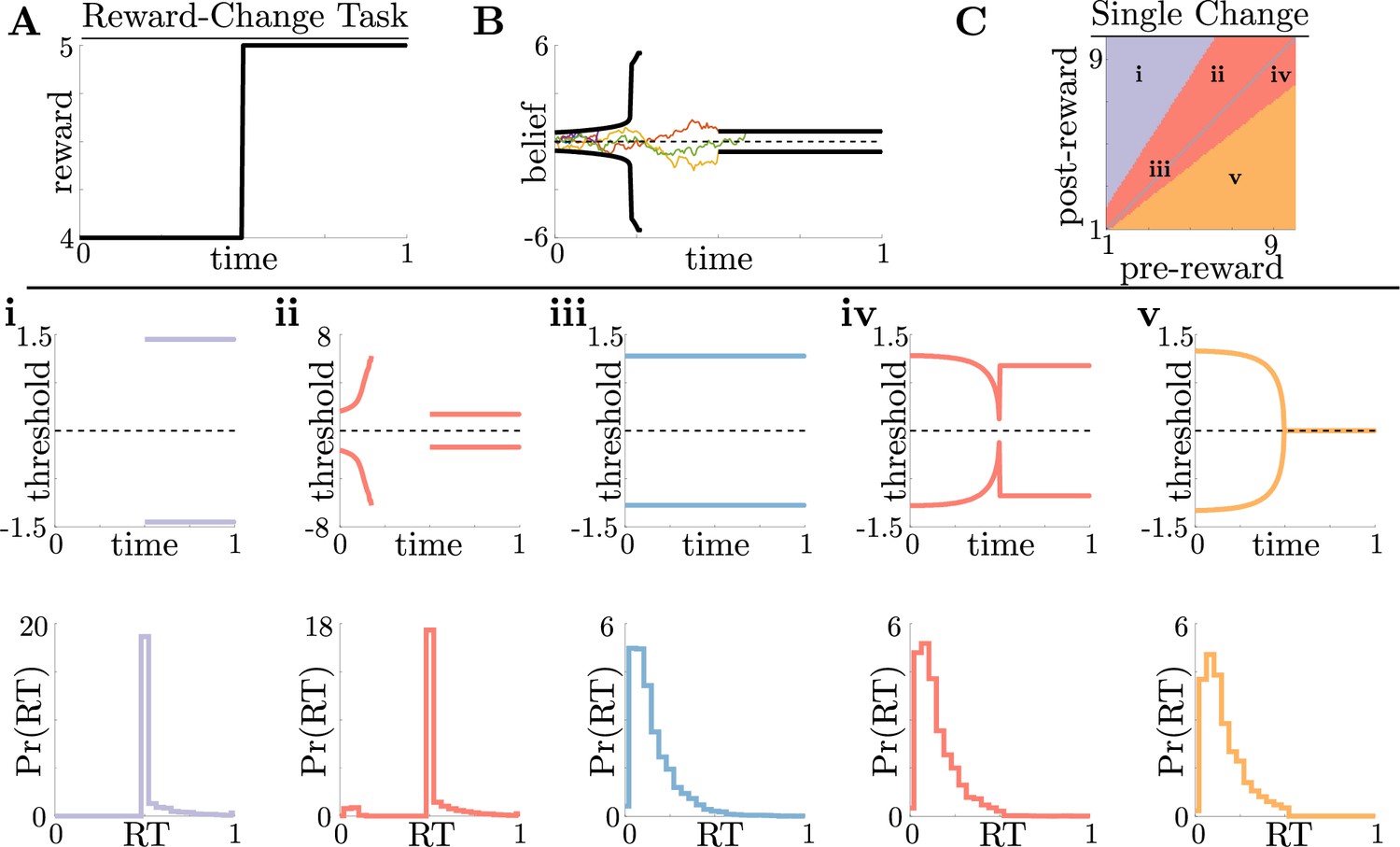
Normative decision rules are characterized by non-monotonic task-dependent motifs.
(A,B) Example reward time series for a reward-change task (black lines in A), with corresponding thresholds found by dynamic programming (black lines in B). The colored lines in B show sample realizations of the observer’s belief. (C) To understand the diversity of threshold dynamics, we consider the simple case of a single change in the reward schedule. The panel shows a colormap of normative threshold dynamics for these conditions. Distinct threshold motifs are color-coded, corresponding to examples shown in panels i-v. (i-v): Representative thresholds (top) and empirical response distributions (bottom) from each region in C. During times at which thresholds in the upper panels are not shown (e.g., in i), the thresholds are infinite and the observer will never respond. For all simulations, we take the incremental cost function , punishment , evidence quality , and inter-trial interval .
Figure 2—figure supplement 1
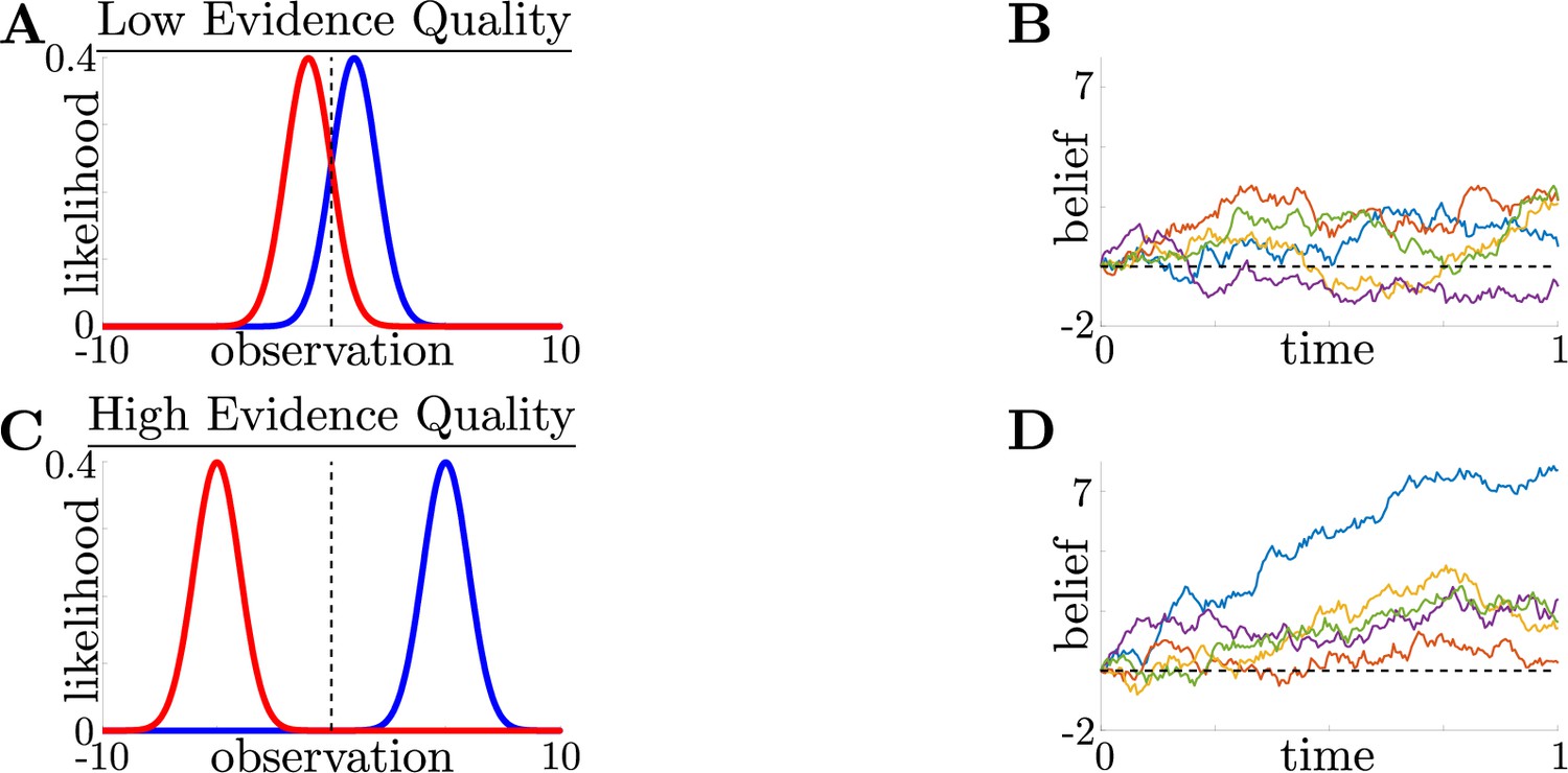
Impact of evidence quality on belief and difficulty.
Evidence quality impacts observation distinguishability and task difficulty. (A) Likelihood functions for environmental states (i.e., possible choices) (blue) and (red) in a low evidence quality task (), where we define , a scaled signal-to-noise ratio, as the evidence quality. (B) Observer belief (LLR of accumulated evidence) in a low evidence quality task, with several belief realizations superimposed. C,D: Same as A and B, but for a high evidence quality task ().
Figure 2—figure supplement 2

Normative thresholds for reward-change task with multiple changes.
Normative decision thresholds exhibit multiple motifs for multiple reward changes. (A,B) Example reward time series for a reward-change task (black lines in A), with corresponding thresholds found by dynamic programming (black lines in B). The colored lines in B show sample realizations of the observer’s belief. Similar changes in reward (boxed regions) produce similar motifs in threshold dynamics.
Figure 2—figure supplement 3
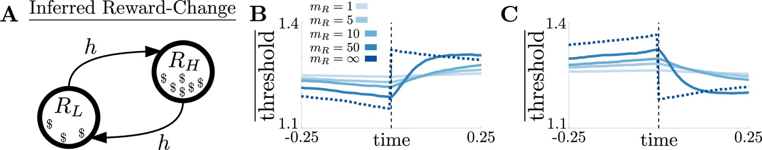
Threshold dynamics in the inferred reward-change task.
Threshold dynamics in the inferred reward change task track piecewise constant dynamics. (A) Markov process governing reward states with rewards and symmetric transition (hazard) rate between states. (B) Change point-triggered average of normative thresholds for a high-to-low reward change. Several values of reward inference difficulty are superimposed (legend). Colored dotted line corresponds to the thresholds for an infinite task, and vertical black dashed line shows the time of the reward switch. (C) Same as B, but for a low-to-high reward change. For both B and C, the rewards are, the state evidence quality is, and the hazard rate is .
Figure 3 with 1 supplement
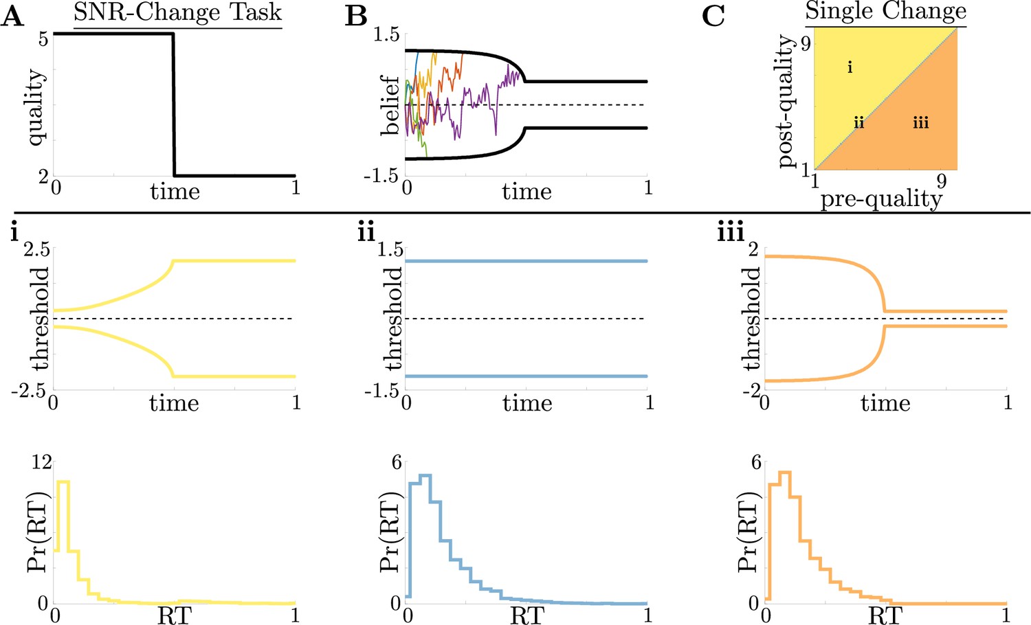
Dynamic-quality task does not exhibit non-monotonic motifs.
(A,B) Example quality time series for the SNR-change task (A), with corresponding thresholds found by dynamic programming (B). Colored lines in B show sample realizations of the observer’s belief. As in Figure 2, we characterize motifs in the threshold dynamics and response distributions based on single changes in SNR. (C) Colormap of normative threshold dynamics for a known reward schedule task with a single quality change. Distinct dynamics are color-coded, corresponding to examples shown in panels i-iii. (i-iii): Representative thresholds (top) and empirical response distributions (bottom) from each region in C. For all simulations, we take the incremental cost function , reward , punishment , and inter-trial interval .
Figure 3—figure supplement 1

Normative thresholds for SNR-change task with multiple changes.
Normative decision thresholds change monotonically when anticipating SNR changes. A,B: Example quality time series for the SNR-change task with multiple changes (A), with corresponding thresholds found by dynamic programming (B). Colored lines in (B) show sample realizations of the observer’s belief. Similar changes in quality (boxed regions) produce similar motifs in threshold dynamics.
Figure 4 with 3 supplements

Benefits of adaptive normative thresholds compared to heuristics.
(A) Reward rate for the noisy Bayesian (NB) model, constant-threshold (Const) model, and UGM for the reward-change task, where all models are tuned to maximize performance with zero sensory noise () and zero motor noise (); in this case, the NB model is equivalent to the optimal normative model. Model reward rates are shown for different pre-change rewards , with post-change reward set so that to keep the average total reward fixed (see Materials and methods for details). Low-to-high reward changes (dotted line) produce larger performance differentials than high-to-low changes (dashed line). (B) Absolute reward rate differential between NB and alternative models, given by for different pre-change rewards. Legend shows which alternate model was used to produce each curve. (C) Reward rates of all models for reward-change task with as both observation and response-time noise is increased. Noise strength for each model is given by , are and were the maximum strengths of and we considered (See Figure 4—figure supplement 1C for reference). Filled markers correspond to no noise, moderate noise, and high noise strengths. D,E,F: Response distributions for (D) NB; (E) Const; and (F) UGM models in a low-to-high reward environment with . In each panel, results derived for several noise strengths, corresponding with filled markers in C, are superimposed, with lighter distributions denoting higher noise. Inset in D shows normative thresholds obtained from dynamic programming. Dashed line shows time of reward increase. For all simulations, we take the incremental cost function , punishment , and evidence quality .
Figure 4—figure supplement 1
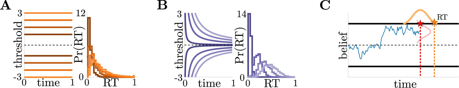
Heuristic model and noise schematics.
Heuristic observer models and noise filters. (A) Constant threshold (Const) model in belief-space (left), with associated RT distributions (right). Several versions of model are superimposed (gradient). (B) Threshold dynamics of the UGM (left), with associated RT distributions (right). The UGM uses a low-pass filtered version of the normative LLR as its belief and dilates this belief linearly in time; this is equivalent to hyperbolically-collapsing decision thresholds (see Materials and methods). (C) Schematic of noise generation processes, describing possible sources of performance decreases. Gaussian noise with standard deviation is added to belief (red) and with standard deviation (motor noise) added to response times (orange).
Figure 4—figure supplement 2

Model performance for high-to-low reward switch.
All models perform similarly in high-to-low reward switches. (A) Reward rates of all models for low-to-high reward changes, with , (dashed line in Figure 4A) at different noise strengths. Filled markers correspond to no noise, moderate noise, and high noise strengths. (B,C,D) Response distribution for (B) NB, with inset showing normative thresholds obtained from dynamic programming; (C) Const; and (D) UGM model in a high-to-low reward environment; several noise strengths, corresponding to filled markers in A, are superimposed, with lighter distributions denoting higher noise.
Figure 4—figure supplement 3

Model performance for decomposed noise strengths.
Effects of belief and motor noise on model performance. (A) Reward rates of NB model (left), Const model (center), and UGM (right) for different values of belief and motor noise strengths in a low-to-high reward switch. Increasing belief noise strength causes performance to decrease substantially, while increasing motor noise strength has little effect on performance. To better visualize performance decreases, we take a slice through the performance surface at a fixed motor noise strength (arrow label in far left panel). (B) Reward rates of each model for different values of belief noise strength and motor noise strength fixed at 0.125 (arrow label in A). (C,D) Same as A,B, but for a high-to-low reward switch.
Figure 5 with 1 supplement
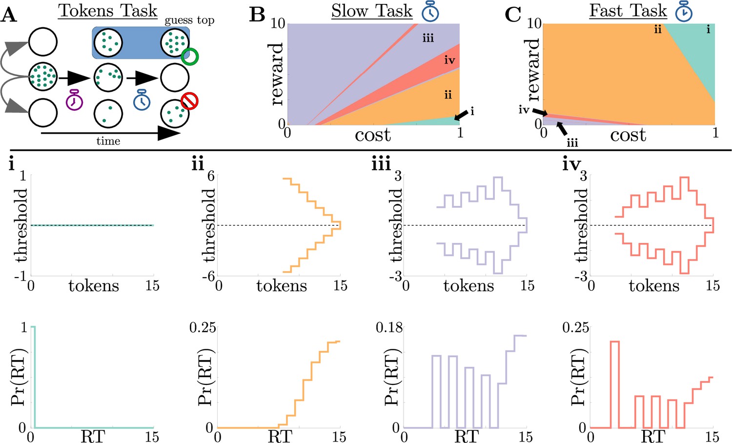
Normative strategies for the tokens task exhibit various distinct decision threshold motifs with sharp, non-monotonic changes.
(A) Schematic of the tokens task. The subject must predict which target (top or bottom) will have the most tokens once all tokens have left the center target (see text for details). (B) Colormap of normative threshold dynamics for the ‘slow’ version of the tokens task in reward-evidence cost parameter space (i.e., as a function of and from Equation 3, with punishment set to –1). Distinct dynamics are color-coded, with different motifs shown in i-iv. (C) Same as B, but for the ‘fast’ version of the tokens task. (i-iv): Representative thresholds (top) and empirical response distributions (bottom) from each region in (B,C). Thresholds are plotted in the LLR-belief space , where is the state likelihood given by Equation 8. Note that we distinguish iii and iv by the presence of either one (iii) or multiple (iv) consecutive threshold increases. In regions where thresholds are not displayed (e.g., in ii), the thresholds are infinite.
Figure 5—figure supplement 1

Tokens task thresholds in token lead space.
Normative thresholds for tokens task plotted in token lead space. i-iv: Same as Figure 5i-iv, but plotted in “token lead” space instead of LLR space. Here, thresholds are measured as the number of tokens the top target must be ahead of the bottom target to commit to a decision. In this space, non-monotonicity of thresholds in iii and iv is more apparent.
Figure 6 with 2 supplements
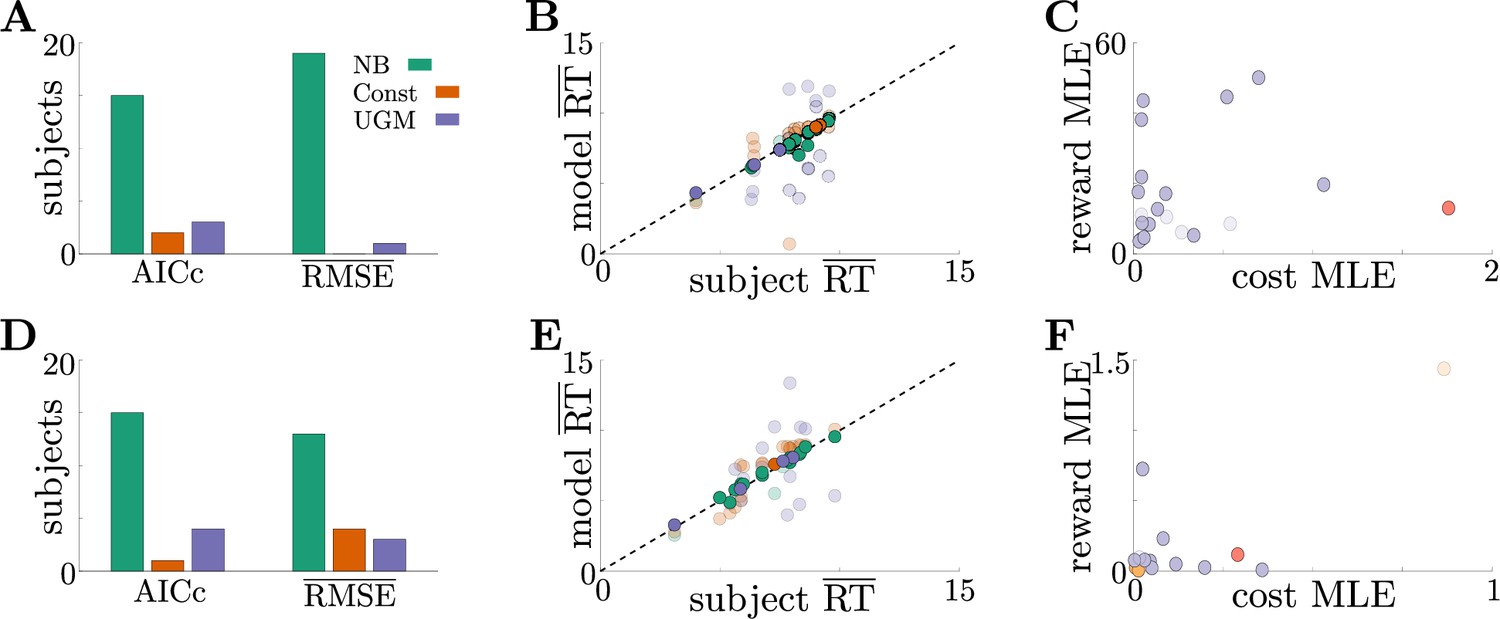
Adaptive normative strategies provide the best fit to subject behavior in the tokens task.
(A) Number of subjects from the slow version of the tokens task whose reponses were best described by each model (legend) identified using corrected AIC (left) and average trial-by-trial RMSE (right). (B) Comparison of mean RT from subject data in the slow version of the tokens task (-axis) to mean RT of each fit model (-axis) at maximum-likelihood parameters. Each symbol is color-coded to agree with its associated model. Darker symbols correspond to the model that best describes the responses of a subject selected using corrected AIC. The NB model had the lowest variance in the difference between predicted and measured mean RT (NB var: 0.13, Const var: 3.11, UGM var: 5.39). (C) Scatter plot of maximum-likelihood parameters and for the noisy Bayesian model for each subject in the slow version of the task. Each symbol is color-coded to match the threshold dynamics heatmap from Figure 5B. Darker symbols correspond to subjects whose responses were best described by the noisy Bayesian model using corrected AIC. (D-F) Same as A-C, but for the fast version of the tokens task. The NB model had the lowest variance in the difference between predicted and measured mean RT in this version of the task (NB var: 0.22, Const var: 0.82, UGM var: 5.32).
Figure 6—figure supplement 1

Summary of model fits.
Best- and worst-quality fits for each model. (A) Best fits, measured using AICc, for the NB model (left), Const model (center), and UGM (right). Black trace shows subject data, and colored trace shows the maximum-likelihood model fit. Each plot shows the Kullback-Leibeler (KL) divergence between the subject data and the fitted response distribution (see Materials and methods for details). (B) Same as A, but for the worst fits for each model.
Figure 6—figure supplement 2

Fitted posterior for each model parameter for NB model.
Example NB posterior for subject tokens task data. (A–D) Fitted posterior from the NB model for reward (A), cost (B), sensory noise (C), and motor noise (D) for a single representative subject. The top row (red) shows the model posterior for slow task, whereas the bottom row (blue) shows the model posterior for the fast task. Note the different scales for the same parameter in different versions of the task. Shaded regions show the approximate 95% credible interval for each marginal posterior. Vertical dashed lines show the MLE values for each parameter, calculated from the full joint posterior.
Tables
Table 1
List of model parameters used for analyzing tokens task response time data.
| NB: | Reward Cost Sensory Noise Motor Noise | Const: | Threshold Sensory Noise Motor Noise | UGM: | Threshold Scale Gain Sensory Noise Time Constant Motor Noise |
Additional files
Download links
A two-part list of links to download the article, or parts of the article, in various formats.
Downloads (link to download the article as PDF)
Open citations (links to open the citations from this article in various online reference manager services)
Cite this article (links to download the citations from this article in formats compatible with various reference manager tools)
Normative decision rules in changing environments
eLife 11:e79824.
https://doi.org/10.7554/eLife.79824


