Disentangling the rhythms of human activity in the built environment for airborne transmission risk: An analysis of large-scale mobility data
- Department of Biology, Georgetown University, United States
Figures
Figure 1 with 4 supplements
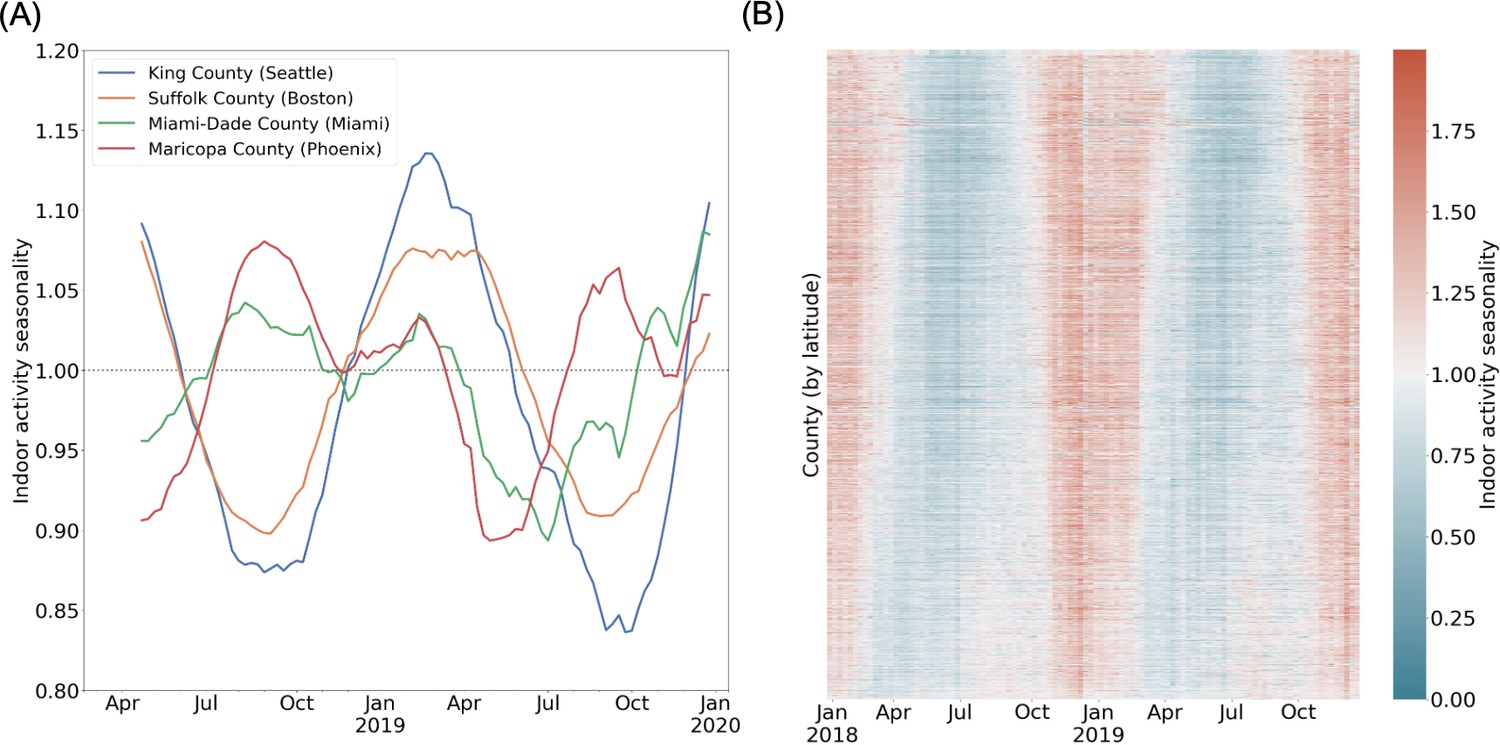
Spatio-temporal heterogeneity in indoor activity seasonality.
(A) Case studies to highlight varying trends in indoor activity seasonality during 2018 and 2019: King County and Suffolk County (in the northern United States) have high indoor activity in the winter months and a trough in indoor activity in the summer months. Miami-Dade and Maricopa County (in the southern United States) see moderate indoor activity in the winter and may have an additional peak in indoor activity during the summer. We apply a rolling window mean for visualization purposes. (B) A heatmap of the indoor activity seasonality metric for all US counties by week for 2018 and 2019. Counties are ordered by latitude. We see significant spatiotemporal heterogeneity with distinct trends in the summer versus winter seasons.
Figure 1—figure supplement 1
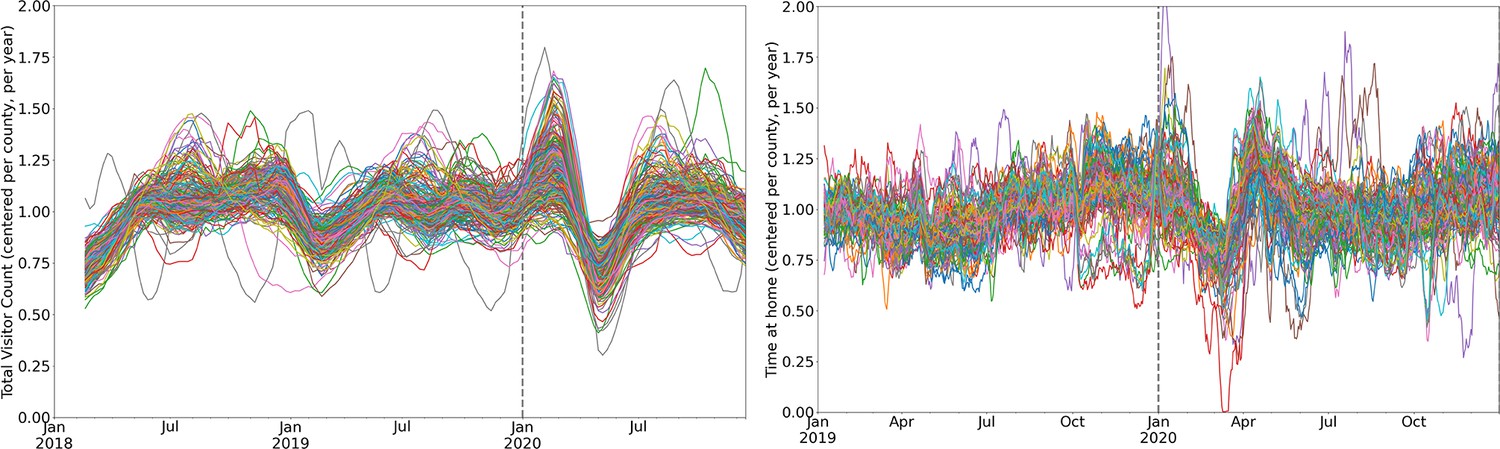
Other measures of mobility are not highly seasonal.
Top: Using the Safegraph Weekly Patterns dataset (https://docs.safegraph.com/docs/weekly-patterns), we show total (all non-home locations) visitor counts for a random sample of 310 counties (10% of all US counties). Overall mobility does not appear to be highly seasonal. Bottom: Using the Safegraph Social Distancing Metrics dataset (https://docs.safegraph.com/docs/social-distancing-metrics), we show time spent at home for a random sample of 310 counties (10% of all US counties). While home locations are not included in our indoor activity metric, time spent at home does not appear to be highly seasonal.
Figure 1—figure supplement 2
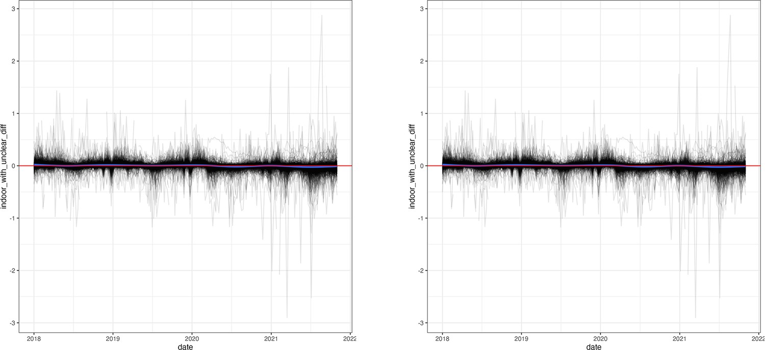
We demonstrate the effect of the ‘unclear’ locations on the indoor activity seasonality.
In the left panel, we show the difference in if all ‘unclear’ locations were to be classified as indoor. In the right panel, we show the difference if if all ‘unclear’ locations are classified as outdoor.
Figure 1—figure supplement 3
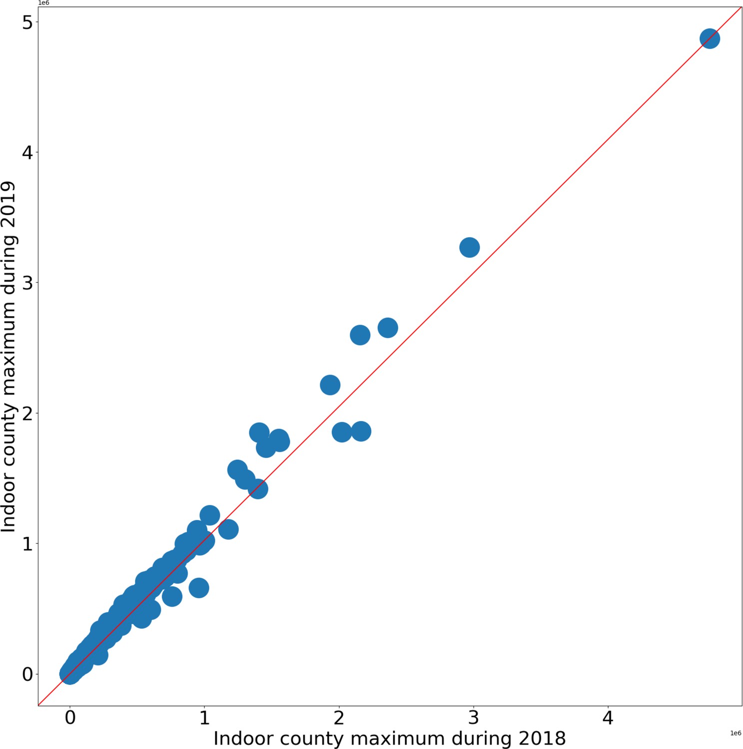
We show that the maximum number of visits used in the definition of the metric is highly comparable in 2018 and 2019.
Figure 1—figure supplement 4
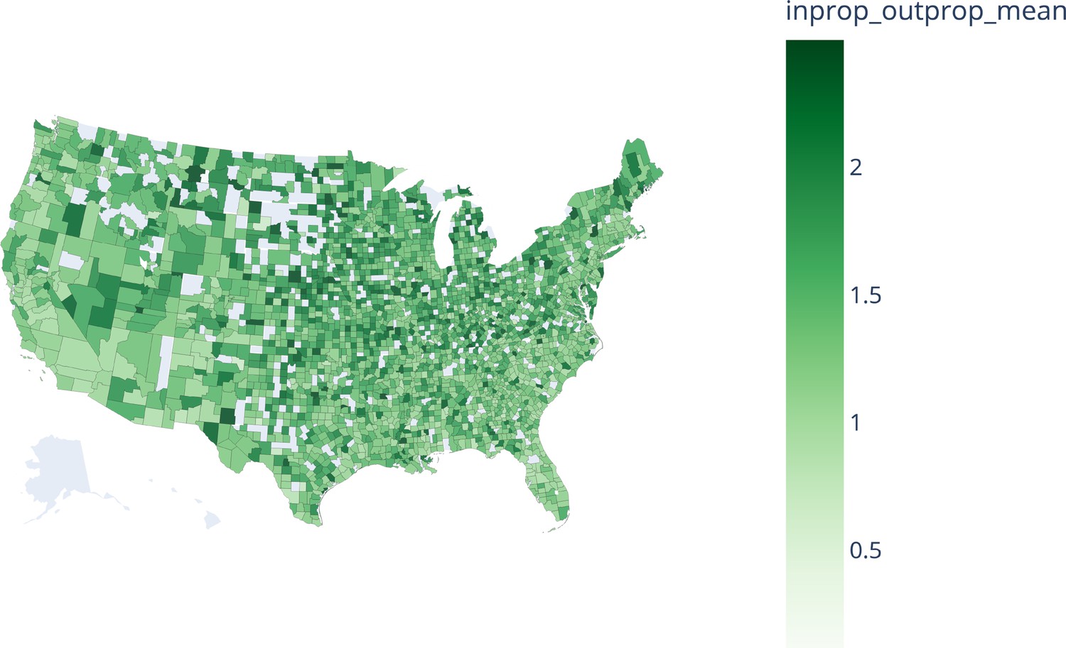
The mean proportion of indoor/outdoor activity () in 2018 displays no latitudinal gradient and is relatively homogeneous across counties; outliers of mean ≥ 2.5 are removed.
Figure 2 with 5 supplements
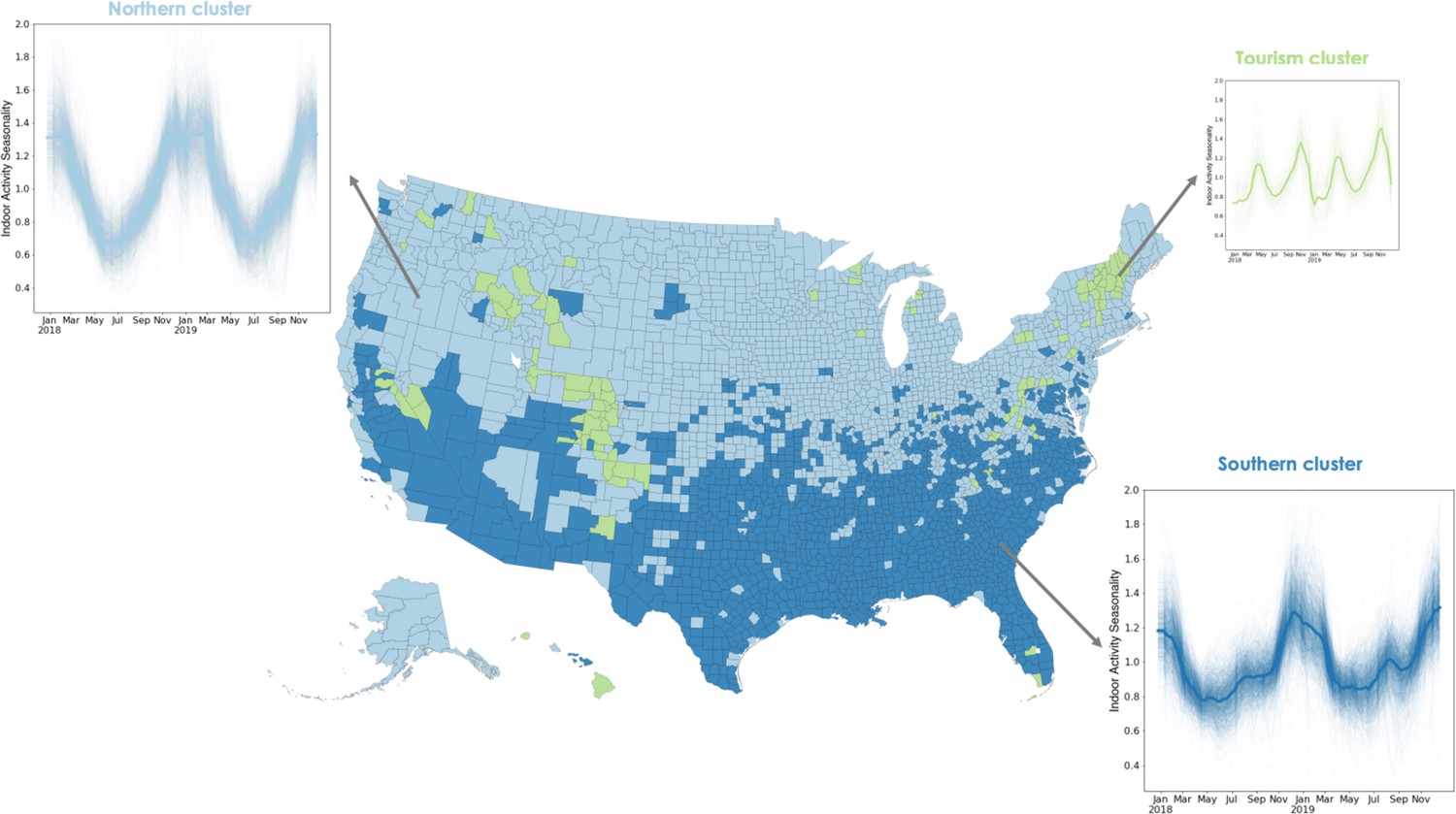
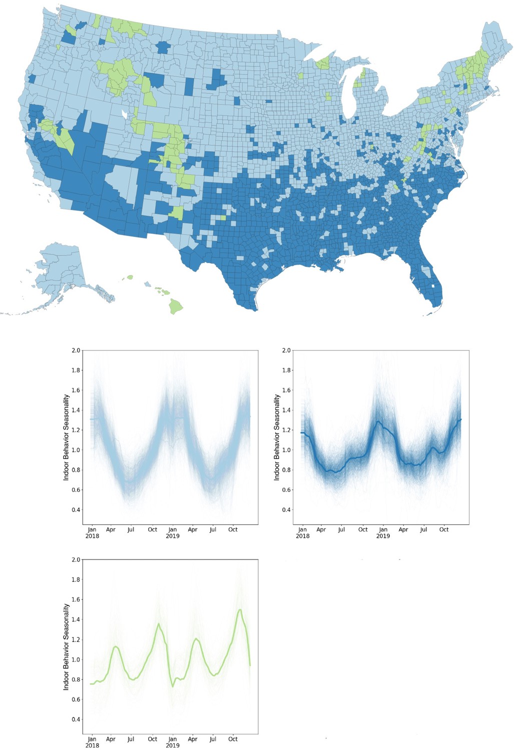
Using a time series clustering approach on the indoor activity time series for each US county, we identify groups of counties that experience similar trends in indoor activity.
Locations in the northern cluster (light blue) follow a single peak pattern with the highest indoor activity occurring every winter. Locations in the southern cluster (dark blue) experience two peaks in indoor activity each year, one in the winter and a second, smaller one in the summer. The third cluster also experiences two peaks not matching environmental conditions, but potentially corresponding to winter or other tourism areas. We apply a rolling window mean to the time series for visualization purposes.
Figure 2—figure supplement 1
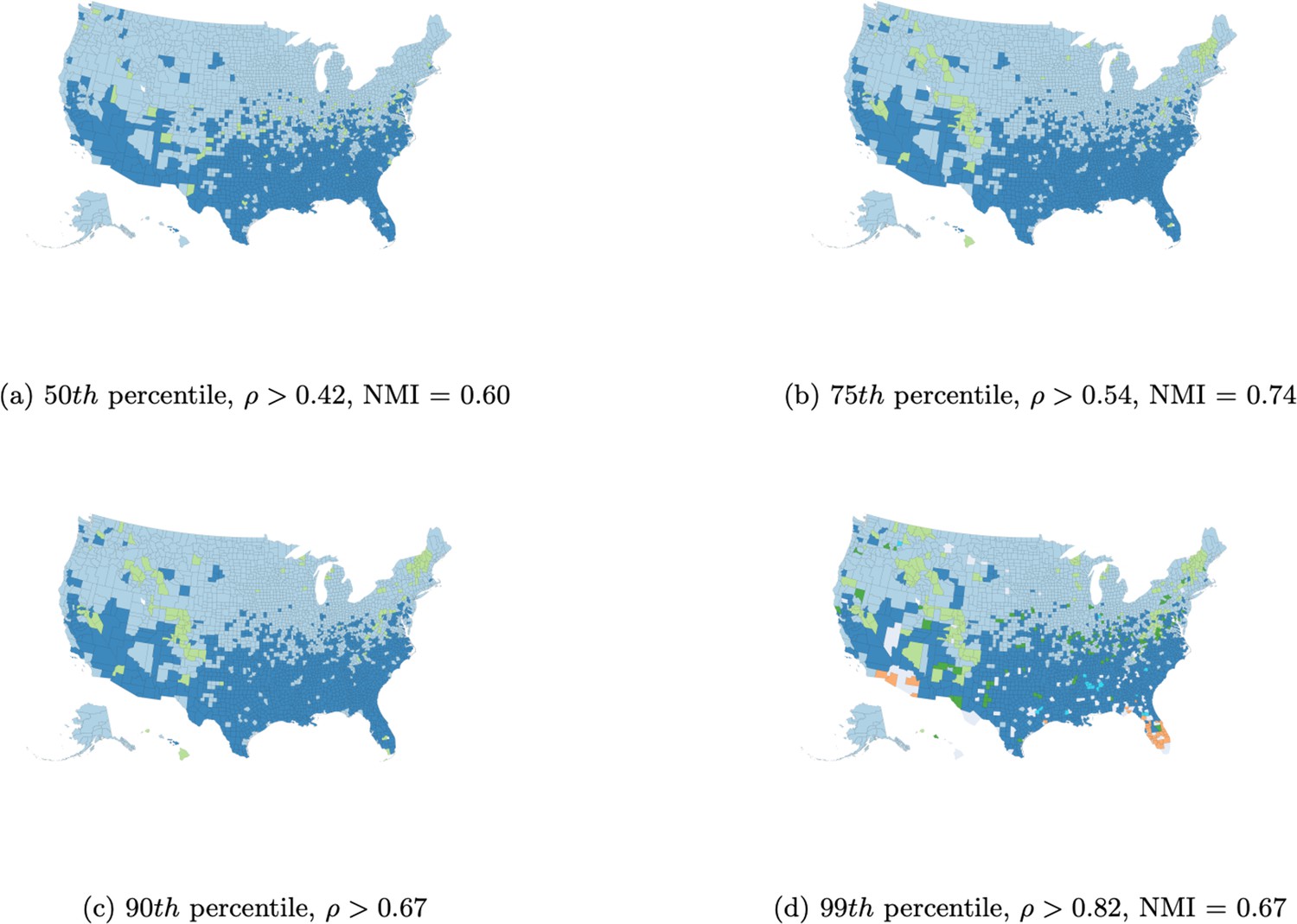
We illustrate the impact of the correlation threshold on the clustering results (without post-processing).
For each panel, we list the percentile for time series correlations used as the threshold, the corresponding correlation value (), and the normalized mutual information between each partition and the partition with the 90th percentile threshold (corresponding to the partition presented in Figure 2).
Figure 2—figure supplement 2

Using data on temperature and rainfall from NOAA’s North American Regional Reanalysis (Mesinger et al., 2006), we find that indoor activity (sigma) is moderately anticorrelated with both temperature and humidity.
Temperature and humidity are strongly correlated in all three clusters (Pearson’s ). Across the three clusters, indoor activity is moderately associated with temperature (). Likewise, indoor activity is moderately anticorrelated with humidity ().
Figure 2—figure supplement 3

Comparison of indoor activity clusters to climate clusters.
(A) The IECC climate zones are based on temperature, humidity, and rainfall in each county and govern the type of building material and amount of ventilation required in a building (International Code Council, 2015). (B) The consistency between the two primary clusters of indoor activity identified by our analysis and the IECC climate zones. Treating the IECC climate zones as ‘ground truth,’ we quantify the ability of our indoor activity clusters to predict the IECC climate zones. We achieve this by collapsing the partitions into two clusters each (the tourism cluster is grouped with the northern cluster in the indoor activity clustering; and IECC climate zones 1/2/3 are grouped into one cluster and zones 4/5/6/7 into another cluster). Our indoor activity clusters have a 0.72 F1-score, with a precision of 0.92 and a recall score of 0.59 with the IECC zones.
Figure 2—figure supplement 4
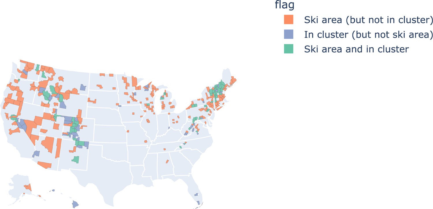
The third indoor activity cluster displays some correlation with areas of increased tourism, including US ski areas in western and northeastern states, potentially contributing to off-season activity increases.
Most areas in the cluster are either in a ski area or neighbor a ski area, with some parts of Hawaii and Florida being clear outliers of this pattern and suggesting other types of tourism lead to similar behavioral seasonality.
Figure 2—figure supplement 5
We show the results of time series clustering based on a hierarchical clustering method using Ward linkage and Euclidean distance, implemented using scipy.cluster in Python.
This partition has high similarity to the network-based clustering algorithm results that we illustrate in Figure 2: normalized mutual information = 0.56 with 89% of counties matching on cluster identity.
Figure 3 with 2 supplements
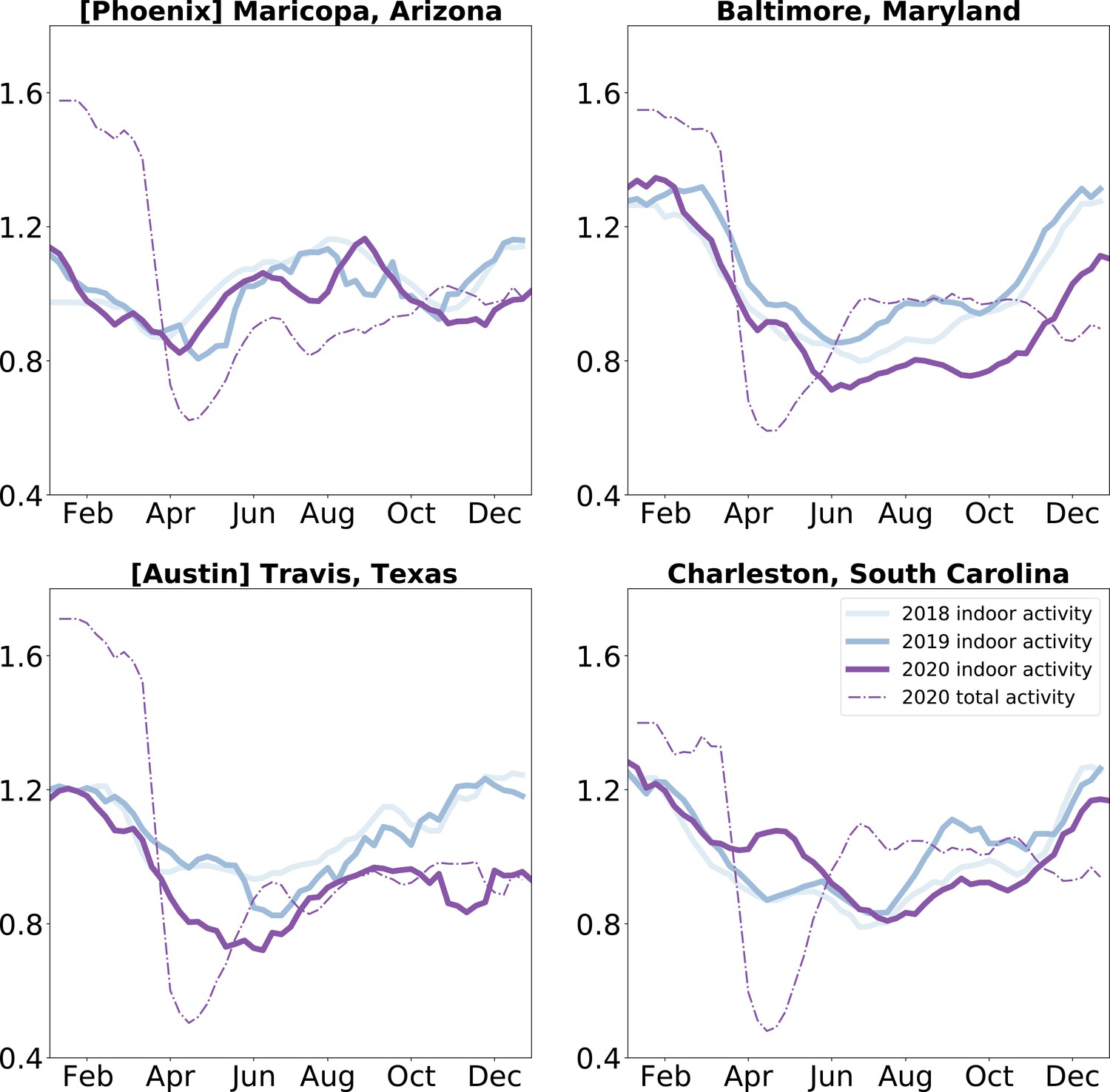
Indoor activity during the COVID-19 pandemic was shifted: We compare indoor activity trends in the baseline years of 2018 and 2019 to the pandemic year 2020 in four case study locations.
We find that most locations saw a shift in their indoor activity patterns, while others (such as Maricopa County) did not. We also find that while overall activity was diminished uniformly during the Spring of 2020, indoor activity decreased in some locations (Travis County, Texas and Baltimore County, Maryland) and increased in others (Charleston County, South Carolina). We apply a three week rolling window mean to the time series for visualization purposes.
Figure 3—figure supplement 1
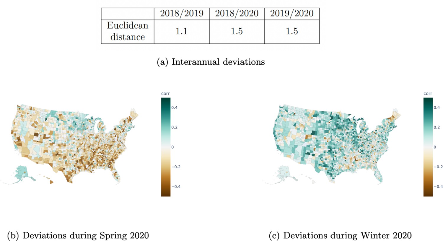
Deviations in 2020 indoor activity from baseline.
Top: Euclidean distance between indoor activity time series in corresponding years for each county, averaged over all counties. The 2020 time series show a higher deviation from each of the baseline years than the two baseline years do from each other. Bottom: We illustrate the mean difference in indoor activity at baseline (defined as the average of 2018 and 2019) and 2020 for two time periods: (a) Week 10 to Week 20 in spring 2020 during the initial lockdown period for COVID-19. (b) Week 44 to Week 52 in winter 2020 during the first winter surge of COVID-19. Positive mean differences suggest more outdoor activity in 2020 than at baseline and negative mean differences suggest more indoor activity in 2020 than at baseline.
Figure 3—figure supplement 2
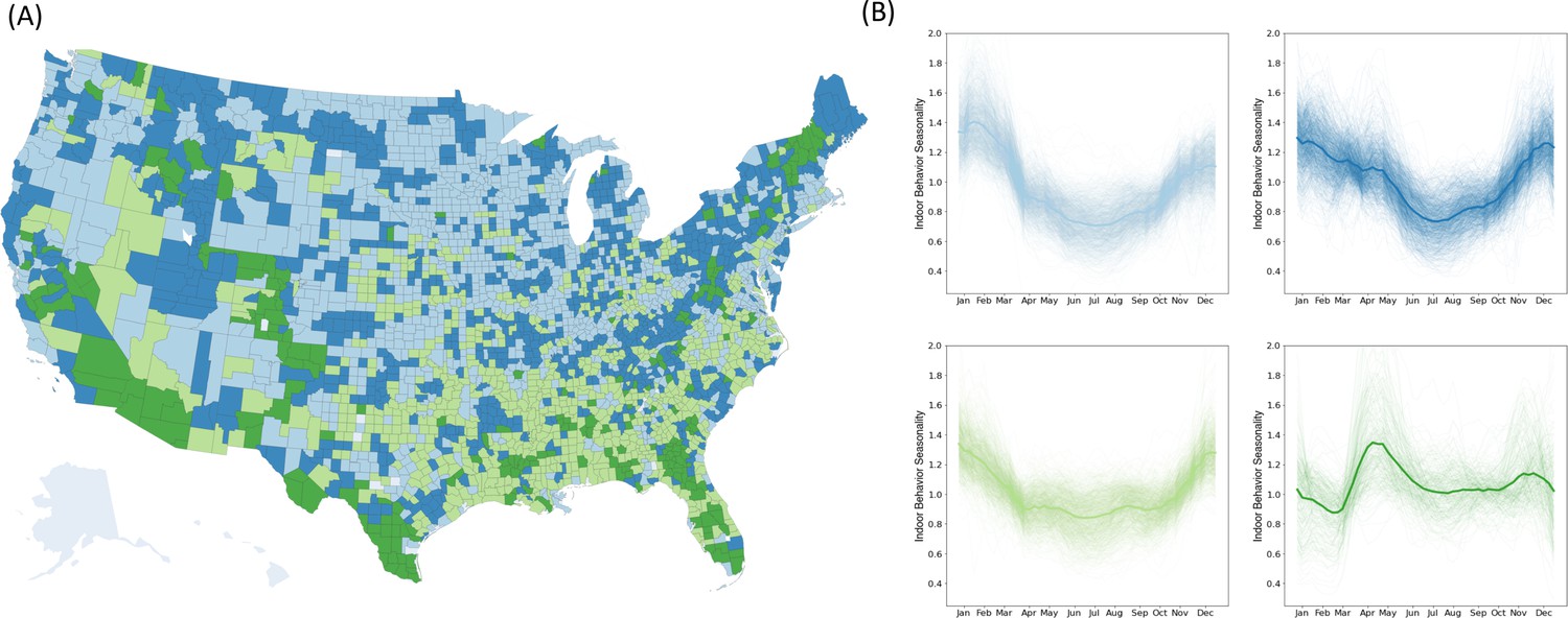
Indoor seasonality clusters during 2020.
(A) Indoor seasonality during 2020 can be clustered into four groups, although clusters are more geographically fragmented than in previous years. (B) Time series for 2020 indoor seasonality clusters display heterogeneous trends that were not apparent in previous years, with some clusters more variable than others.
Figure 4 with 3 supplements

Incorporating seasonality in epidemiological models.
(A) Sine curves fit to the 2018 and 2019 time series data (analogous to seasonal forcing model components) fit the northern cluster better than the southern cluster, with a markedly poorer fit for the southern cluster’s second summer peak. (B) Regional seasonal forcing models display variation in patterns of disease incidence omitted by a non-seasonal model, but even region-level seasonal forcing does not fully capture within-cluster county-level variation.
Figure 4—figure supplement 1

Parameters of the sinusoidal model fits.
Top: Inferred parameters for the sinusoidal model fits of the indoor activity data for the northern and southern clusters show a similar frequency, but the greater amplitude and shorter phase in the southern cluster. Values displayed are mean parameter estimates. Standard errors for all parameters are smaller than 5e−3 and thus are not displayed. Bottom: We show the estimated parameters for the parameters of the sine curve fits to the Northern and Southern clusters as well as the difference between the parameter estimates. The period is in units of time (weeks). The amplitude matches the units of . The phase is in units of time (weeks).
Figure 4—figure supplement 2
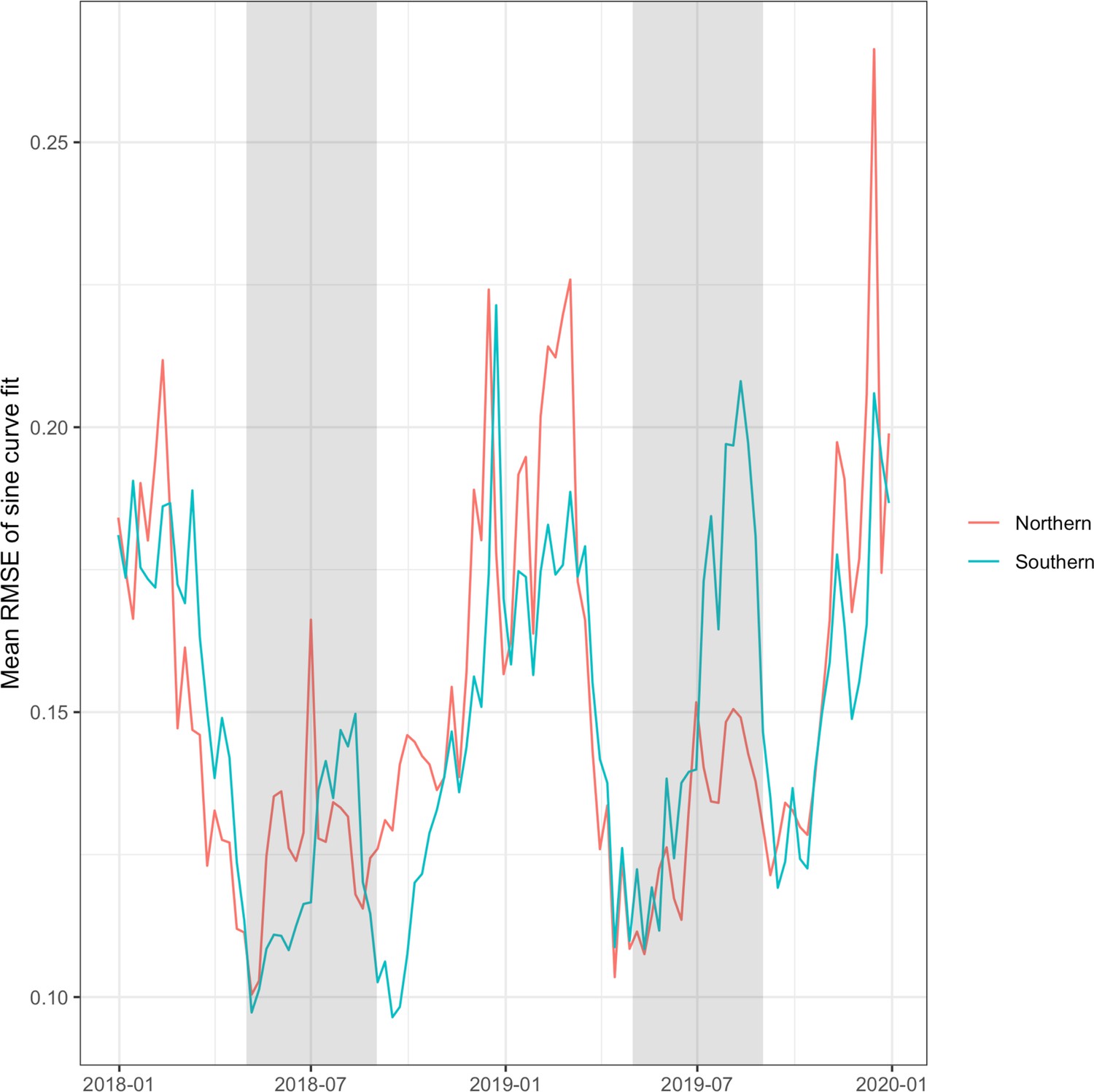
Model performance as measured by the root mean square error of the sine curve fit to the cluster averaged over counties within the cluster.
The summer period between March and September is highlighted in light gray to emphasize the summer months.
Figure 4—figure supplement 3
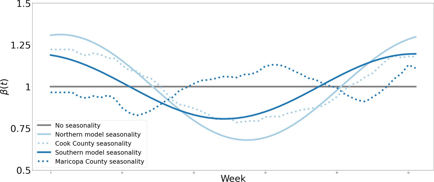
The seasonal forcing functions () we used in the epidemiological model.
The non-seasonal model (gray) shows no variation in transmission risk over time. We model northern seasonality via a sinusoidal model fit to the northern indoor activity data (light blue solid) and via the empirically-measured indoor seasonality from a county in the northern cluster (Cook County, light blue dotted). We model southern seasonality via a sinusoidal model fit to the southern indoor activity data (dark blue solid) and via the empirically-measured indoor seasonality from a county in the northern cluster (Maricopa County, dark blue dotted).
Additional files
Download links
A two-part list of links to download the article, or parts of the article, in various formats.
Downloads (link to download the article as PDF)
Open citations (links to open the citations from this article in various online reference manager services)
Cite this article (links to download the citations from this article in formats compatible with various reference manager tools)
Disentangling the rhythms of human activity in the built environment for airborne transmission risk: An analysis of large-scale mobility data
eLife 12:e80466.
https://doi.org/10.7554/eLife.80466


